Sentinel 2-Based Nitrogen VRT Fertilization in Wheat: Comparison between Traditional and Simple Precision Practices - MDPI
←
→
Page content transcription
If your browser does not render page correctly, please read the page content below

agronomy
Article
Sentinel 2-Based Nitrogen VRT Fertilization in Wheat:
Comparison between Traditional and Simple
Precision Practices
Marco Vizzari * , Francesco Santaga and Paolo Benincasa
 Department of Agricultural, Food, and Environmental Sciences, University of Perugia, 06121 Perugia, Italy;
 francescosaverio.santaga@unipg.it (F.S.); paolo.benincasa@unipg.it (P.B.)
 * Correspondence: marco.vizzari@unipg.it; Tel.: +39-075-585-6059

 Received: 8 April 2019; Accepted: 23 May 2019; Published: 30 May 2019

 Abstract: This study aimed to compare standard and precision nitrogen (N) fertilization with variable
 rate technology (VRT) in winter wheat (Triticum aestivum L.) by combining data of NDVI (Normalized
 Difference Vegetation Index) from the Sentinel 2 satellite, grain yield mapping, and protein content.
 Precision N rates were calculated using simple linear models that can be easily used by non-specialists
 of precision agriculture, starting from widely available Sentinel 2 NDVI data. To remove the effects
 of not measured or unknown factors, the study area of about 14 hectares, located in Central Italy,
 was divided into 168 experimental units laid down in a randomized design. The first fertilization
 rate was the same for all experimental units (30 kg N ha−1 ). The second one was varied according to
 three different treatments: 1) a standard rate of 120 kg N ha−1 calculated by a common N balance; 2) a
 variable rate (60–120 kg N ha−1 ) calculated from NDVI using a linear model where the maximum
 rate was equal to the standard rate (Var-N-low); 3) a variable rate (90–150 kg N ha−1 ) calculated from
 NDVI using a linear model where the mean rate was equal to the standard rate (Var-N-high). Results
 indicate that differences between treatments in crop vegetation index, grain yield, and protein content
 were negligible and generally not significant. This evidence suggests that a low-N management
 approach, based on simple linear NDVI models and VRT, may considerably reduce the economic and
 environmental impact of N fertilization in winter wheat.

 Keywords: NDVI; remote sensing; GIS; precision farming; variable rate technology; yield mapping;
 protein content

1. Introduction
     In recent decades, population growth and the expanding demand of agricultural products
for multiple purposes have constantly increased the environmental pressures on land and water
resources. Worldwide concern of citizens and governments on environmental issues, together with
the availability of improved and cost-effective methodologies and tools for spatial data acquisition,
analysis, and modeling, have promoted the development of precision agriculture (PA) techniques.
PA is based on innovative system approaches that use a combination of various technologies such as
Geographic Information System (GIS), Global Navigation Satellite System (GNSS), computer modeling,
Remote Sensing (RS), variable rate technology (VRT), yield mapping and advanced information
processing for timely in-season and between season crop management [1].
     Currently, a wide range of satellite data is available that varies in terms of acquisition cost,
technique (active/passive), spatial resolution, spectral range, and viewing geometry [2]. A recent step
forward was made thanks to the launches of Sentinel-2A (2015) and Sentinel-2B (2017) satellites by
the European Space Agency (ESA), intended for Earth observation and monitoring of land surface

Agronomy 2019, 9, 278; doi:10.3390/agronomy9060278                             www.mdpi.com/journal/agronomy
Agronomy 2019, 9, 278                                                                                 2 of 12

variability. The Sentinel-2 satellites are equipped with a multispectral sensor (MSI) including 13 spectral
bands, with a spatial resolution ranging from 10 m to 60 m, which provides relevant information for
supporting precision agriculture [3]. Images provided by Sentinel-2 satellites are publicly available for
free through the Copernicus Open Access Hub with 5 days temporal resolution averaging (2–3 days in
mid-latitudes), in L1C or L2A processing levels, which make them attractive for time-series analysis
and PA applications. The Level-2A product provides Bottom Of Atmosphere (BOA) reflectance images
derived from the associated Level-1C product, which provides Top Of Atmosphere (TOA) reflectance
images [4].
      Satellite remote sensing of vegetation is mainly based on the green (495–570 nm) and red
(620–750 nm) regions of the visible spectrum, the red-edge (680–730 nm), near and mid infrared bands
(850–1700 nm). These bands are often combined with a range of algebraic formulas to obtain several
Vegetation Indices (VIs) for assessing vegetation status and crop management (see e.g. references [5–7]).
The Normalized Difference Vegetation Index (NDVI) [8], a normalized difference between reflectance of
Red and Near-Infrared (NIR) spectral bands, is still the most used index worldwide because of its ease
of calculation and interpretation. It varies between 0 and 1 in cropped areas, increasing with soil cover,
LAI (Leaf Area Index), chlorophyll content, and plant N-nutritional status (see e.g. references [9–11]).
The NDVI has been widely tested to assess wheat N-nutritional status and yield, with encouraging
results [12–14].
      N is the main nutrient supplied to most crops, including wheat, and may cause environmental
impacts on near-surface and deep aquifers [15]. Increasing the N rate generally increases crop yield
since it increases the grain number and size [16]. However, increasing the N rates reduces the N
uptake efficiency and increases the amount of residual N in the soil which is exposed to leaching
risks [9,17]. Countless studies are available on wheat N nutrition and several of the recent ones have
dealt with precision N fertilization, but most of them propose quite complex approaches that are
not widely adoptable by non-specialists of PA. For example, Bourdin et al. [18] propose a complex
model starting from LAI, estimated by remote sensing, and yields from previous years; Basso et al. [19]
use a crop simulated model (SALUS) based on weather and yields from previous years. Another
approach consists in assessing spatial variability to delineate homogeneous sub-field areas overlapping
various thematic spatial maps (such as yield, soil properties) or applying a multivariate geostatistical
approach of the factors that affect yield and grain quality [20]. In this context Song et al. [21] delineated
management zones on the basis of soil, yield data and remote sensing information derived from
Quickbird imagery. Besides these methods, to improve the use of N prescription maps in PA, various
simplified approaches based on NDVI have also been developed through user-friendly web interfaces
(e.g. CropSAT [22], Agrosat [23], OneSoil [24]) but these approaches can be applied only in specific
areas or lack either quantitative analysis or validation.
      While traditional flat-rate spreaders typically tend to over- or under-apply fertilizers, with VRT
spreaders it is possible to modify the distribution rate according to on-the-go proximal sensors
measuring, in real-time, plant properties or prescription maps derived through more or less advanced
models including various spatial factors (e.g.: vegetation indices, soil variables, yield maps, crop
nutrition status) [25]. However, the majority of precision fertilization approaches are generally
map-based, because on-the-go sensors are too expensive, not sufficiently accurate, or not available [26].
VRT spreaders are subject to errors depending on the technology and the intrinsic characteristics of the
fertilizer [27].
      Grain yield mapping aims at providing or increasing knowledge about the spatial heterogeneity of
yields. This technology is based on the recording of georeferenced yield data thanks to the integration
of different subsystems mounted on the combines [28]: (i) harvest quantity measurement sensors (mass
or volume); (ii) GNSS location sensors; (iii) reference area measurement sensors (working width, speed,
time); (iv) data recording and processing units. To generate yield maps, the harvested quantities are
georeferenced and associated with the corresponding reference area which is calculated by multiplying
the working width by the area length (working speed * time interval). Yield mapping accuracy is
Agronomy 2019, 9, 278                                                                                        3 of 12

      Agronomy 2019, 9, x FOR PEER REVIEW                                                                         3 of 12

      influenced by many factors including flow sensor calibration, combined speed changes, grain flow
 96         While many studies combine VIs (from various remote or proximal sensors) and VRT crop
      variations, grain moisture, and the level of smoothing applied for mapping [29].
 97   fertilization, only a small quantity of research integrates yield mapping sensors, and, to our
            While many studies combine VIs (from various remote or proximal sensors) and VRT crop
 98   knowledge, probably no study has ever combined VIs, VRT fertilization, and yield mapping in a PA
      fertilization, only a small quantity of research integrates yield mapping sensors, and, to our knowledge,
 99   case study and, in particular, to assess the effects of different variable N-rate treatments on winter
      probably no study has ever combined VIs, VRT fertilization, and yield mapping in a PA case study
100   wheat.
      and, in particular, to assess the effects of different variable N-rate treatments on winter wheat.
101         In this framework, this study was aimed at comparing two VRT N fertilization treatments (based
            In this framework, this study was aimed at comparing two VRT N fertilization treatments (based
102   on Sentinel 2) versus a standard flat N rate in terms of crop NDVI trend, grain yield, and protein
      on Sentinel 2) versus a standard flat N rate in terms of crop NDVI trend, grain yield, and protein
103   content. In order to promote the adoption of PA techniques among farmers and non-specialists in
      content. In order to promote the adoption of PA techniques among farmers and non-specialists in
104   PA, a simplified approach, based on free and open-source software, the widely used NDVI, and an
      PA, a simplified approach, based on free and open-source software, the widely used NDVI, and an
105   easily-applicable linear model, was applied to calculate the VRT N fertilization rates.
      easily-applicable linear model, was applied to calculate the VRT N fertilization rates.
106   2.
      2. Materials
         Materials and
                   and Methods
                       Methods

107   2.1.
      2.1. Crop
           Crop Management
                Management and
                           and Experimental
                               Experimental Treatments
                                            Treatments
108        The
           The experiment
                experiment was
                             was carried
                                   carried out
                                           out in
                                               in the
                                                   the cropping
                                                        cropping season
                                                                   season 2017-2018,
                                                                              2017-2018, on
                                                                                          on aa 14
                                                                                                14 ha
                                                                                                    ha plain
                                                                                                        plain field of the
                                                                                                              field of the
109   middle  Tiber valley, near   Deruta, Umbria,    Italy (170  m  a.s.l., 42°95’07’’
                                                                             ◦           N, ◦12°38’18’’  E), provided
      middle Tiber valley, near Deruta, Umbria, Italy (170 m a.s.l., 42 95’07” N, 12 38’18” E), provided by the         by
110   the Foundation   for Agricultural   Education    of Perugia   (Figure    1). The soil  was  loam
      Foundation for Agricultural Education of Perugia (Figure 1). The soil was loam with increasing sandwith  increasing
111   sand  content
      content       from
               from the    the to
                         west   west
                                  the to the
                                      east   eastThe
                                           side.   side.  The climate
                                                       climate           is Mediterranean,
                                                                is Mediterranean,               characterized
                                                                                       characterized     by a drybyseason
                                                                                                                    a dry
112   season between   May   and  September   and   a cold  and  rainy  season    from  October-November
      between May and September and a cold and rainy season from October-November to March-April.               to March-
113   April.
      The     The cropping
          cropping             season 2017–2018
                    season 2017–2018     was unusuallywasrainy
                                                            unusually
                                                               in Decemberrainyand in March,
                                                                                       Decemberwhileand    March, while
                                                                                                     temperatures    were
114   temperatures  were
      generally higher     generally
                        than          higher than
                              the poly-annual       the except
                                                 trend  poly-annual    trendcold
                                                               for a very      except
                                                                                    endfor
                                                                                        of aFebruary
                                                                                              very cold(Figure
                                                                                                         end of 2).
                                                                                                                 February
115   (Figure 2).

116
           Figure 1. Geographical location of the study area and experimental layout. Flat-N (standard rate of
117        Figure 1. Geographical location of the study area and experimental      layout. Flat-N (standard rate of
           120 kg N ha−1  ), Var-N-low (variable rate from 60 to 120 kg N ha−1 ), Var-N-high (variable rate from 90
118        120 kg N ha ),−1
                       −1   Var-N-low (variable rate from 60 to 120 kg N ha ), Var-N-high (variable rate from 90
                                                                            −1
           to 150 kg N ha ).
119        to 150 kg N ha−1).
           The experimental crop was a rainfed winter wheat (Triticum aestivum L., cv. PRR58) sown on
      10 November 2017 at a nominal density of 450 viable seeds m-2 . The previous crop had been pea
      (Pisum sativum Asch et Gr). The crop was managed according to ordinary practices, while weeds
      and diseases were controlled chemically. The N rate was split in two application times in order to
      increase N uptake efficiency, support the formation of yield components and limit N leaching by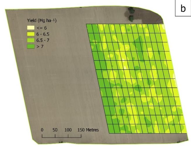
Agronomy 2019, 9, 278 4 of 12
fall-spring rainfall. The first N application (as urea) occurred on 18 January 2018 with 30 kg N ha−1 ,
while the second N fertilization (as urea), occurred on 26 March 2018 and was managed according to
three experimental treatments: 1) a standard rate of 120 kg N ha−1 (Flat-N) derived by an N balance
approach (the relatively high rate is justified by the very rainy winter); 2) a variable rate of 60 to
120 kg N ha−1 , based on NDVI, where the maximum rate was equal to the standard rate (Var-N-low);
3) a variable rate of 90 to 150 kg N ha−1 , based on NDVI, where the medium rate was equal to the
standard rate (Var-N-high). An inverse linear relationship between NDVI and VRT N-rates was
adopted in Var-N-low and Var-N-high on the assumption that NDVI and other correlated VIs (e.g.
NIR/Red simple ratio), before the second N fertilization (7–8 Feekes’ stage), are directly related to
crop N nutritional status [10,13,30]. Thus, the Var-N-high was defined with the aim of keeping the
average N-rate equal to the flat N-rate while optimizing the N fertilization according to the supposed
N nutritional status. The range adopted in Var-N-high represents a variation of ±25% of the flat N rate,
and a ±20% of the total N supplied (including the 30 kg N ha−1 of the first N application), which was
considered as being appropriate to see appreciable effects on wheat yield. The Var-N-low was defined
with the aim of testing a sensible N reduction, the results of which were very important in those areas
where a more eco-compatible approach is required. So, the flat N-rate was considered as the maximum
N level and the −50% of the flat N rate (−40% of the total rate, equal to 90 Kg/ha including the first N
application) was adopted as a lowest reference level based on the evidence from a previous study in
the same2019,
Agronomy location [16].
9, x FOR PEER REVIEW 4 of 12
Rain (long-term) Rain 2017/18 T. (long-term) T. 2017/18
180 25
160
140 20
Temperature (°C)
Rainfall (mm)
120
15
100
80
10
60
40 5
20
0 0
I II III I II III I II III I II III I II III I II III I II III I II III I II III
OCT NOV DEC JAN FEB MAR APR MAY JUN
120
121 Figure 2.2.Monthly
Figure Monthlycumulated
cumulatedrainfall andand
rainfall average temperatures
average per decade
temperatures during the
per decade wheat
during growing
the wheat
122 season 2017–2018 and in the long term (temperature 1951–2018, rainfall 1921–2018).
growing season 2017–2018 and in the long term (temperature 1951–2018, rainfall 1921–2018).
123 To
Theaccount for the crop
experimental possible
wasnot measured
a rainfed or unknown
winter factors,aestivum
wheat (Triticum the 14 ha L.,study area was
cv. PRR58) sown divided
on 10
124 into 168 plots of about 700 square meters each (35 m long, 21 m wide) grouped
November 2017 at a nominal density of 450 viable seeds m-2. The previous crop had been pea (Pisum in 28 zones. The three
125 treatments
sativum Asch were etlaid
Gr).down
The according
crop was to a randomized
managed design
according to with 2 replicates
ordinary practices,per while
treatment
weeds in each
and
126 zone for a total of 56 replicates per treatment in the whole study area (Figure 1). All the
diseases were controlled chemically. The N rate was split in two application times in order to increase precision on-field
127 operations were performed
N uptake efficiency, supportusing a tractor equipped
the formation with a Topcon
of yield components and GNSS
limit Nautomatic
leaching by guide device
fall-spring
128 connected
rainfall. Theto afirst
RealNTime Kinematic
application (as(RTK)
urea)network.
occurredThe variable
on 18 rate2018
January treatments
with 30were kg Nperformed
ha−1, whileusing
the
129 asecond
Sulky 40+ (ECONOV) VRT fertilizer spreader connected through ISOBUS (a
N fertilization (as urea), occurred on 26 March 2018 and was managed according to three widely used software
130 protocol complaint
experimental to ISO 11783
treatments: standard)rate
1) a standard to theofTopcon
120 kgsystem
N ha−1console.
(Flat-N)The console,
derived by after
an Neach VRT
balance
131 fertilization, releases the output of each fertilization map showing the estimated distributed
approach (the relatively high rate is justified by the very rainy winter); 2) a variable rate of 60 to 120 rates.
132 This
kg Noutput was compared
ha−1, based on NDVI, to the prescription
where the maximum map to investigate
rate was equal to thethe accuracy
standard of rate
the N distribution.3)
(Var-N-low);
133 a variable rate of 90 to 150 kg N ha−1, based on NDVI, where the medium rate was equal to the
134 standard rate (Var-N-high). An inverse linear relationship between NDVI and VRT N-rates was
135 adopted in Var-N-low and Var-N-high on the assumption that NDVI and other correlated VIs (e.g.
136 NIR/Red simple ratio), before the second N fertilization (7–8 Feekes’ stage), are directly related to
137 crop N nutritional status [10,13,30]. Thus, the Var-N-high was defined with the aim of keeping the
138 average N-rate equal to the flat N-rate while optimizing the N fertilization according to the supposed
139 N nutritional status. The range adopted in Var-N-high represents a variation of ±25% of the flat N
140 rate, and a ±20% of the total N supplied (including the 30 kg N ha−1 of the first N application), which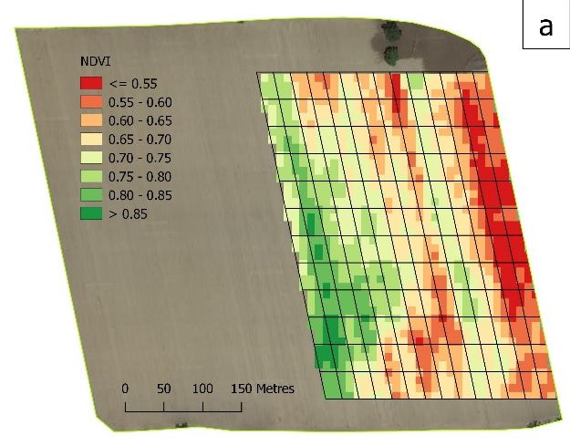
Agronomy 2019, 9, 278 5 of 12
2.2.Agronomy
Calculation
2019, 9,ofx Rates for VRT
FOR PEER Treatments
REVIEW 5 of 12
158 2.2.ACalculation
Level 2AofSentinel-2 image
Rates for VRT collected on 22 March 2018 (i.e., four days before the second
Treatments
fertilization), georeferenced according to WGS84-UTM32, was downloaded from The Copernicus
159 A Level
Open Access 2A NDVI,
Hub. Sentinel-2 image from
calculated collected
bandson422 March
and 2018
8 using QGIS(i.e.,Raster
four calculator
days before the second
(Figure 3a), was
160 fertilization), georeferenced according to WGS84-UTM32, was downloaded from The Copernicus
used for the N rates calculation of the two variable rate treatments. In both cases, a linear relationship
161 Open Access Hub. NDVI, calculated from bands 4 and 8 using QGIS Raster calculator (Figure 3a),
was imposed between the average NDVI value calculated for all experimental units and fertilizer-N
162 was used for the N rates calculation of the two variable rate treatments. In both cases, a linear
rates where the 5◦ percentile of NDVI value corresponded to the minimum fertilizer-N rates (60 or
163 relationship was imposed between the average NDVI value calculated for all experimental units and
90 kg N ha−1 ) and the 95◦ percentile of NDVI value corresponded to the maximum fertilizer-N rate
164 fertilizer-N rates where the 5° percentile of NDVI value corresponded to the minimum fertilizer-N
(120 or 150 kg N ha−1 ) (Figure 3b). All the data processing and analysis were carried out using QGIS
165 rates (60 or 90 kg N ha−1) and the 95° percentile of NDVI value corresponded to the maximum
166 software, version
fertilizer-N 2.18.12
rate (120 64bit
or 150 kg[31]
N haand MS Excel
−1) (Figure 3b).2016. Average
All the NDVI values
data processing were calculated
and analysis using
were carried
167 theout
SAGA grid statistics for the polygons algorithm included in the QGIS processing
using QGIS software, version 2.18.12 64bit [31] and MS Excel 2016. Average NDVI values were framework.
168 Tocalculated
simplify this step,
using thepixels
SAGAoverlapping
grid statisticsthe
forborder of the algorithm
the polygons experimental plotsin
included were not excluded
the QGIS from
processing
169 theframework.
calculation. To assess the effect of these pixels, average NDVI values were compared
To simplify this step, pixels overlapping the border of the experimental plots were not with those
170 obtained
e while considering only non-overlapping pixels.
171
172
173 Figure
Figure 3. 3.(a)
(a)NDVI
NDVI calculated
calculated from Level
Level 2A
2A Sentinel-2
Sentinel-2image
imagecollected
collectedonon2222March
March2018; (b)(b)
2018;
174 Prescription N map developed by integrating
Prescription N map developed by integrating the the three different experimental treatments.
different experimental treatments.
175 2.3.2.3.
Determination
DeterminationofofNDVI
NDVI
176 ToTomonitor
monitor and
andcompare
comparethe theNDVI
NDVIof of experimental treatments,all
experimental treatments, allrelevant
relevantlevel
level
2A2A Sentinel-2
Sentinel-2
177 images
images with
with nonocloud
cloudcover
coverononthe
thestudy
study area,
area, were collected
collectedfrom
from22 22March
Marchtotothethebeginning
beginning of of
thethe
178 senescence.Average
senescence. AverageNDVI
NDVI values
valueswerewerecalculated
calculated forfor
each plotplot
each using the SAGA
using the SAGAgrid statistics for thefor
grid statistics
179 thepolygons
polygons algorithm
algorithmincluded
includedin the QGIS
in the processing
QGIS framework.
processing framework.Six to Six
ninetoS2nine
pixels
S2 fell within
pixels fell each
within
180 experimental
each experimental unit. To To
unit. highlight
highlightpossible differences
possible differencesbetween
between the the
effects of of
effects thetheexperimental
experimental
181 treatments
treatments whileconsidering
while consideringdifferent
differentcrop
crop vigor
vigor status
status before
beforethethesecond
secondNNfertilization, thethe
fertilization, NDVI
NDVI
182 time series analysis was performed by classifying plots according to three NDVI classes (NDVI0.68;
time series analysis was performed by classifying plots according to three NDVI classes (NDVI ≤ ≤ 0.68;
183 0.68
0.68 < NDVI≤≤0.79;
< NDVI 0.79;NDVI
NDVI > > 0.79),
0.79), as
as revealed
revealedby bythe
theS2S2image
imagefromfrom 2222
March.
March.
184 2.4.2.4. DeterminationofofGrain
Determination GrainYield
Yieldand
andProtein
Protein Content
Content
185 Harvestwas
Harvest wascarried
carriedout
outonon 26
26 June
June 2018
2018 using
using aa combined
combinedharvester
harvesterClaas
ClaasLexion
Lexion780–740
780–740
186 equipped
equipped with a Topcon YieldTrakk system (processing data from the optical sensor measuring grain
with a Topcon YieldTrakk system (processing data from the optical sensor measuring grain
187 mass flow and moisture sensors), which produced a georeferenced yield map as an ESRI polygon
mass flow and moisture sensors), which produced a georeferenced yield map as an ESRI polygon
188 shapefile. The combine harvester had a cutting width of 7.50 m and was equipped with a tilt sensor
shapefile. The combine harvester had a cutting width of 7.50 m and was equipped with a tilt sensor to
189 to correct the effect of slope on the sensor readings. An initial on-field calibration was performed on
190 correct the effect of slope on the sensor readings. An initial on-field calibration was performed on the
the combine to adjust for the actual working width and measure the unit weight of grain, which was
191 combine to adjust for the actual working width and measure the unit weight of grain, which was used
used by the system to convert the measured mass flow (l/s) to Mg.
192 by the system to convert
The output the measured
shapefile containingmass
the flow (l/s) to Mg.yield data was intersected with the
georeferenced
193 experimental units to calculate the average yield expressed in Mg ha−1 which was used for the
194 subsequent analysis. To produce an easy-to-read yield map, the shapefile was converted to a 5 m
Agronomy 2019, 9, 278 6 of 12
The output shapefile containing the georeferenced yield data was intersected with the experimental
units to calculate
Agronomy 2019, 9, xthe
FORaverage yield expressed in Mg ha−1 which was used for the subsequent analysis.
PEER REVIEW 6 of 12
To produce an easy-to-read yield map, the shapefile was converted to a 5 m resolution raster. Subsequent
195 resolution raster. Subsequent gaussian kernel smoothing, based on a 50 m search radius, produced
gaussian kernel smoothing, based on a 50 m search radius, produced the final yield map.
196 the final yield map.
Protein content was measured on 20 June 2018 (i.e., six days before final harvest). To reduce
197 Protein content was measured on 20 June 2018 (i.e., six days before final harvest). To reduce the
the number of samples, the sampling scheme was defined according to the three classes of NDVI
198 number of samples, the sampling scheme was defined according to the three classes of NDVI
previously defined for a total of 36 field samples, then merged two by two to obtain 18 lab samples,
199 previously defined for a total of 36 field samples, then merged two by two to obtain 18 lab samples,
which were analyzed according to the official Kjeldahl method, a widely used chemical procedure for
200 which were analyzed according to the official Kjeldahl method, a widely used chemical procedure
201 thefor
quantitative determination
the quantitative of protein
determination content
of protein in food,
content feed,feed,
in food, feed feed
ingredients and and
ingredients beverages [32].
beverages
202 [32].
3. Results
203 3. The
Results
NDVI values on 22 March show within-field differences mainly associated with the west-east
204 texturalThe
gradient
NDVI (Figure 3a).
values on 22Average
March show NDVI values including
within-field overlapping
differences pixels with
mainly associated withplot
the borders
west-
205 differ only slightly from those obtained while excluding these pixels (0.015
east textural gradient (Figure 3a). Average NDVI values including overlapping pixels with in average absolute
plot
206 value, 0.011differ
borders St. Dev.). According
only slightly fromto those
the linear model
obtained usedexcluding
while for N-rates calculation,
these theseindifferences
pixels (0.015 average
207 correspond only to0.011
absolute value, 2.6 kg/ha (1.8 St.
St. Dev.). Dev.) forto
According Var-N-low
the lineartreatment
model used andfor
2.6N-rates
kg/ha (2.1 St. Dev.) these
calculation, for the
208 Var-N-high treatment.
differences correspond only to 2.6 kg/ha (1.8 St. Dev.) for Var-N-low treatment and 2.6 kg/ha (2.1 St.
209 A comparison
Dev.) between
for the Var-N-high the prescription map and the Sulky output (Figure 4a) shows that the
treatment.
210 A comparison
correlation between the between
prescribedthe prescription
rate and the map and the supplied
rate actually Sulky output (Figure
by the 4a) shows
VRT machine that the
within each
211 plot was very good (R = 0.91) (Figure 4b), with only a little bias which resulted in smoothing the
correlation between 2
the prescribed rate and the rate actually supplied by the VRT machine within
212 each plot
extremes, was very
raising good (R²
the lower rates= 0.91) (Figure 4b),
and lowering thewith onlyones
higher a little bias1).
(Table which resulted in smoothing
213 the extremes, raising the lower rates and lowering the higher ones (Table 1).
214
215 Figure
Figure 4. (a)
4. (a) Comparisonbetween
Comparison betweenprescription
prescriptionmap
map and
and the distributed
distributedSulky
Sulkyoutput.
output.(b)
(b)Scatter plot
Scatter plot
216 between
between thethe prescribed
prescribed and
and distributedrate
distributed ratewithin
withineach
each plot.
plot.
217 Table 1. Amounts
Table 1. Amountsofof
NNprescribed
prescribedand
andsupplied
supplied with
with the secondN
the second Napplication
applicationininthe
the three
three treatments:
treatments:
218 Flat-N (standard rate of 120 kg N ha −1 ),−1Var-N-low (variable rate from 60 to 120 kg N ha−1 ),−1Var-N-high
Flat-N (standard rate of 120 kg N ha ), Var-N-low (variable rate from 60 to 120 kg N ha ), Var-N-
219 (variable rate from
high (variable 90from
rate to 150
90 kg N ha
to 150
−1 ).
kg N ha−1).
AverageNN prescribed Average N supply Average
Average Δ St. Dev.
Treatments Average N supply Average ∆ St. Dev. −1
Treatments prescribed
(Kg N ha−1) (Kg N ha−1(Kg N ha −1) Δ (%)
) ∆ (%) (Kg N haN
(Kg −1 ha
) )
Flat-N (Kg N ha−1 ) 120.0 116.5 −1.3% 0.03
Flat-N
Var-N-low 120.0 90.2 116.5 95.4 −1.3% 5.4% 0.03 0.06
Var-N-low
Var-N-high 90.2 120.5 95.4 117.0 5.4% −3.0% 0.06 0.05
Var-N-high 120.5 117.0 −3.0% 0.05
220 After the second fertilization, the trend of NDVI, considering the three vigor classes previously
221 defined, was not affected by fertilization treatments (Figure 5). In the portion of the field where the
222 NDVI was already high on 22 March (class III—about 0.85), all treatments showed a further moderate
223 increase up to over 0.9, while in the portion of the field where NDVI was low (class I—just over 0.6),
224 all treatments showed an increase up to 0.85 in about one month, and nearly 0.9 later on. As expected,Agronomy 2019, 9, 278 7 of 12
After the second fertilization, the trend of NDVI, considering the three vigor classes previously
defined, was not affected by fertilization treatments (Figure 5). In the portion of the field where the
NDVI was already high on 22 March (class III—about 0.85), all treatments showed a further moderate
increase up to over 0.9, while in the portion of the field where NDVI was low (class I—just over 0.6),
all treatments
Agronomy 2019, 9,showed an increase
x FOR PEER REVIEW up to 0.85 in about one month, and nearly 0.9 later on. As expected,
7 of 12
an intermediate trend can be observed for treatments with NDVI falling within class II. Thus, whatever
225 an intermediate
the crop vigor statustrend can
was onbe observed
March 22nd,for with NDVI
all treatments reached falling
a high NDVI within class II.
one month Thus,
after the
226 whatever the crop vigor status
second N application (Figure 5). was on March 22 nd, all treatments reached a high NDVI one month
227 after the second N application (Figure 5).
0.95
0.9
III
0.85
0.8
NDVI
0.75 II
0.7
1
2
0.65 I
3
0.6
228 3/22 3/29 4/5 4/12 4/19 4/26 5/3 5/10 5/17 5/24
229 Figure NDVItime
Figure 5. NDVI timeseries
series analysis,
analysis, considering
considering the the
threethree
vigorvigor classes
classes as identified
as identified in theinS2the S2
image
230 image of March 22nd (I: NDVI ≤ 0.68; II: 0.68 < NDVI ≤ 0.79; III: NDVI > 0.79),
of March 22 (I: NDVI ≤ 0.68; II: 0.68 < NDVI ≤ 0.79; III: NDVI > 0.79), for the three N fertilization
nd for the three N
231 fertilization
treatments: treatments: 1) Flat-Nrate
1) Flat-N (standard (standard
of 120 kg rate
N of
ha120
−1 kgVar-N-low
); 2)
−1
N ha ); 2)(variable
Var-N-low (variable
rate from 60rate from
to 120 kg60N
232 to
ha120
−1); 3) N ha−1 ); 3) (variable
kgVar-N-high Var-N-highrate(variable
from 90rate from
to 150 kg 90 to −1
N ha 150). kg N ha ).
−1
Grain Yield and Quality
233 3.3. Grain Yield and Quality
The yield map used for the quantitative analysis is shown in Figure 6a, while the generalized
234 The yield map used for the quantitative analysis is shown in Figure 6a, while the generalized
version used only for visual analysis purposes is shown in Figure 6b. The three treatments did not
235 version used only for visual analysis purposes is shown in Figure 6b. The three treatments did not
differ significantly for total yield (Table 2) and no relationship was found between the N rate and
236 differ significantly for total yield (Table 2) and no relationship was found between the N rate and
yield (R2 = 0.087). Similarly, no correlation was found between N treatments and protein content
237 yield (R² = 0.087). Similarly, no correlation was found between N treatments and protein content (R²
(R2 = 0.001). However, the slight difference in protein content observed between Flat-N and Var-N-low
238 = 0.001). However, the slight difference in protein content observed between Flat-N and Var-N-low
(Table 2) was statistically significant (p = 0.02) even though it was not agronomically relevant. Finally,
239 (Table 2) was statistically significant (p = 0.02) even though it was not agronomically relevant. Finally,
grain yield was weakly correlated to NDVI at any time of NDVI measurements (Table 3).
240 grain yield was weakly correlated to NDVI at any time of NDVI measurements (Table 3).
Table 2. Grain yield and protein content for the three N fertilization treatments: Flat-N (standard rate
of 120 kg N ha−1 ), Var-N-low (variable rate from 60 to 120 kg N ha−1 ), Var-N-high (variable rate from
90 to 150 kg N ha−1 ).
Average Yield St. Dev. Yield (Mg Average Protein St. Dev. Protein
Treatment
(Mg ha−1 ) ha−1 ) Content (%) Content (%)
Flat-N 6.74 0.36 9.4 0.31
Var-N-low 6.73 0.39 8.9 0.37
Var-N-high 6.76 0.38 9.2 0.48
241
242 Figure 6. (a) yield map used for quantitative analysis; (b) generalized version of yield map.0.7
1
2
0.65 I
3
Agronomy 2019, 9, 278 8 of 12
0.6
228 3/22 3/29 4/5 4/12 4/19 4/26 5/3 5/10 5/17 5/24
Table 3. Correlation between yield and NDVI at any time of NDVI measurement plotted over all of the
229 Figure 5. NDVI time series analysis, considering the three vigor classes as identified in the S2 image
168 plots.
230 of March 22nd (I: NDVI ≤ 0.68; II: 0.68 < NDVI ≤ 0.79; III: NDVI > 0.79), for the three N fertilization
231 treatments: 1) Flat-N (standard rate of Date R2
120 kg N ha−1); 2) Var-N-low (variable rate from 60 to 120 kg N
232 ha−1); 3) Var-N-high (variable rate from 90
22 Marto 150 kg N ha −1).
0.29
6 Apr 0.26
233 3.3. Grain Yield and Quality
21 Apr 0.24
234 The yield map used for the quantitative analysis is shown in Figure 6a, while the generalized
29 Apr 0.19
235 version used only for visual analysis purposes is shown in Figure 6b. The three treatments did not
11 May 0.19
236 differ significantly for total yield (Table 2) and no relationship was found between the N rate and
237 10 May
yield (R² = 0.087). Similarly, no correlation 0.18 N treatments and protein content (R²
was found between
238 = 0.001). However, the slight difference 26 in
May 0.27
protein content observed between Flat-N and Var-N-low
239 (Table 2) was statistically significant (p31
= 0.02)
May even though0.26
it was not agronomically relevant. Finally,
240 grain yield was weakly correlated to NDVI at any time of NDVI measurements (Table 3).
241
242 Figure
Figure 6. (a) yield
6. (a) yield map
map used
used for
for quantitative
quantitative analysis;
analysis; (b)
(b) generalized
generalized version
version of
of yield
yield map.
map.
4. Discussion
243
Our study investigated the differences between a flat N fertilization rate and two variable rates
defined through a simplified method based on Sentinel-2 NDVI collected a few days before the second
fertilization. One of the two variable rates was aimed at drastically reducing the overall N input
(Var-N-low), the other one was aimed at maintaining the same overall input (Var-N-high) as in the
flat rate (Flat-N), i.e., 120 kg N ha−1 while optimizing the N fertilization according to the supposed N
nutritional status. Our results show that a VRT approach with a lower overall N rate may be more
efficient, giving same grain yield and quality (Table 2) with a lower N input (Table 1). This result is
consistent with the evidence of Raun et al. [33] which reports that the VRT method improves the NUE
(Nitrogen Use Efficiency) by 15% compared to a flat rate. In vulnerable contexts, as in the study area,
the N-rate reduction results environmentally and economically very relevant since it could reduce
water pollution (still a critical issue in Umbria and all over the world) and decrease expenditures on N.
However, differently from our case study, a Var-N-low treatment could determine a lower protein grain
content. In this regard, the economic trade-off between lower N costs and reduced yield value due to
lower grain protein content could be calculated by the farmers using their local costs and prices. Indeed,
the treatment Var-N-low differed from the other two treatments by only about 20 kg N ha−1 on average,
which was supposed to be not so important compared to the total amount available (i.e., about 160 vs
180 kg ha−1 ), accounting for the residual N left by the previous pea crop (likely around 30 kg N ha−1 )
and the amount of N supplied with the first mineral N application (30 kg N ha−1 ). It is worth noting
that about 180 kg ha−1 of available N was in line with the usual practice adopted by farmers in the
Tiber valley of Umbria and adequate, if not limiting, in view of the high yielding potential of this areaAgronomy 2019, 9, 278 9 of 12
(6–8 tons grains ha−1 ). Nonetheless, the rainy fall-spring of 2017–2018 caused a relevant N loss from
the soil, thus, in this case, a difference of 20 kg N ha−1 was expected to make a difference. Several
reasons can be addressed to explain the lack of difference among treatments. The main one is that
crop development was not associated to N availability but to the soil textural gradient, with NDVI
values tendentially as lower as higher appeared the sand content in the soil. In such a condition, and
considering the rainy season, forcing the N rate in plots with low NDVI (i.e., with higher sand content)
resulted in losing N (mainly by leaching) without affecting yield. As reported by Asseng & Turner [34],
NUE is mainly influenced by soil and rain. Thus, in our case, the N rate increase did not translate
in a NUE increase as this was probably limited by the other factors. This would justify that, in some
cases, the N rate should be directly related to the NDVI [35], i.e., increased where NDVI is higher and
decreased where NDVI is lower, on the assumption that lower NDVI values could prove that other soil
characteristics, besides N availability, are not suitable for allowing high yields. For example, a soil
with low water retention is not suitable in case of dry grain filling periods (as it is in Mediterranean
areas) due to water shortage and thus lower yields whatever the N availability [36–38]. The similar
time course of NDVI observed in all the three treatments, distinguishing three different vigor status
before the second fertilization (Figure 5), also proves that N was not the limiting factor, or at least, the
20 kg N ha−1 of difference among treatments was not relevant for crop NDVI.
The weak correlation between grain yield and NDVIs at any date of monitoring (R2 always below
0.3) appears in contrast with the evidence of Sultana et al. [12] and Liu et al. [39] which show high
correlation between NDVI and yield, especially for NDVI recorded during the milky-grain vegetative
stage. However, the NDVI recorded in our experiment from 21 April onwards was quite high for all
treatments, whereas it is known that the correlation with yield stands only when a wide range of NDVI
is considered [16].
As discussed above, the textural gradient likely affected yield through N and water availability,
more than the N fertilization treatments. This assumption is supported by the case study of
Basso et al. [19] who observed a high correlation between yield and pedological conditions, in particular
soil water capacity. Also, Zhao et al. [40] reported that fertilization, as well as the availability of water,
significantly affected the content of wheat proteins, even though the latter was more influent, especially
for those cultivars characterized by an intermediate protein content. Probably, further splitting the
rate, with a third application at the end of shooting, would have prevented some N loss and increased
the grain protein content [41], which was quite low compared to the standard of our cultivar. Again,
the low protein content can be ascribed to the rainy season, as it was widespread for the harvest of
2018 in Umbria and all-over Central Italy.
Concerning the prescription map used in the study, including the overlapping pixels with plot
borders in average NDVI calculation simplifies the GIS procedures without generating agronomically
meaningful N-rates differences. Because of the high variability within field zones and among plots,
the map could be considered as a kind of stress test for the VRT device. The very little differences
between prescribed and distributed rates (Table 2) suggest that this technology is suitable for precision
fertilization even with highly detailed prescription maps. The highlighted differences are clearly due
to small plot size and random allotment of treatments. As a result, the VRT machine was subjected to
abrupt rate variations due to the short time available to adapt the opening of the distribution valve.
The simple linear approach to calculate a N prescription map proposed in this research, even
though requiring average GIS skills could be effective for VRT adoption by non-specialist farmers.
Coherently with other similar experiences [22–24], to improve the overall usability of the method
by non-specialists in PA and allow further validations and tuning, all the RS data management and
GIS calculation could be implemented in an user-friendly web-GIS application where the user could
upload (or digitize on aerial data) his own fields, choose the S2 NDVI reference date, and decide the
most suitable approach for defining the N rate. NDVI S2 data could be conveniently accessed through
the Sentinel Hub platform API [42].Agronomy 2019, 9, 278 10 of 12
Concerning the integration of NDVI from Sentinel 2, VRT fertilization, and yield mapping in
PA, our experience confirms that these technologies, thanks also to both the web-based applications
for calculating satellite-based prescription maps [22–24] and the user-friendly interfaces of system
consoles, could be ordinarily used even in small or medium-sized farms. However, a preliminary
cost-benefit analysis and a start-up training and support by a PA expert is often necessary.
5. Conclusions
Our results regarding crop vegetation index, grain yield, and protein content indicate that the
adoption of a low-N management approach, based on simple linear models and VRT, may considerably
reduce the economic and environmental impact of nitrogen fertilization in winter wheat. However, the
rainfed nature of winter wheat in Mediterranean environments may cause unpredictable yield and
quality variations depending on climatic trends and soil properties due to their effects on both soil
nitrogen and water availability. In this view, VRT nitrogen fertilization can only partially mitigate the
heterogeneity of production determined by such environmental factors. The alternative approach of
providing a nitrogen supply proportional to the crop NDVI deserves to be considered when factors
other than N fertilizer rate come into play, as it is with sandy soils where NDVI and yield may be
limited by low N and water retention. Despite the known limitations of predictions and prescriptions
based on remoted sensed vegetation indices, their use provides relevant information about within-field
and between-fields variability. This information can support the implementation of crop fertilization
management approaches based on GNSS/RTK and VRT technologies to replace the traditional flat-N
rate, which provides results that are neither economically nor environmentally sustainable.
Author Contributions: All the Authors conceived the research and designed the methodology; M.V. and F.S.
applied the methodology and analyzed the data; P.B. supervised the research; all the Authors wrote the paper.
Funding: This research was developed within the framework of the project “RTK 2.0—Prototipizzazione di una
rete RTK e di applicazioni tecnologiche innovative per l’automazione dei processi colturali e la gestione delle
informazioni per l’agricoltura di precisione”—RDP 2014–2020 of Umbria—Meas. 16.1—App. 84250020256.
Acknowledgments: The authors wish to thank Mauro Brunetti of the Foundation for Agricultural Education of
Perugia for his very helpful and valuable support.
Conflicts of Interest: The authors declare no conflict of interest.
References
1. Liaghat, S.; Balasundram, S.K. A review: The role of remote sensing in precision agriculture. Am. J. Agric.
Biol. Sci. 2010, 5, 50–55. [CrossRef]
2. Oza, S.R.; Panigrahy, S.; Parihar, J.S. Concurrent use of active and passive microwave remote sensing data for
monitoring of rice crop. Int. J. Appl. Earth Obs. Geoinf. 2008, 10, 296–304. [CrossRef]
3. Zheng, Q.; Huang, W.; Cui, X.; Shi, Y.; Liu, L. New Spectral Index for Detecting Wheat Yellow Rust Using
Sentinel-2 Multispectral Imagery. Sensors 2018, 18, 868. [CrossRef]
4. Copernicus Open Access Hub. Available online: https://scihub.copernicus.eu/ (accessed on 4 April 2019).
5. Silleos, N.G.; Alexandridis, T.K.; Gitas, I.Z.; Perakis, K. Vegetation indices: Advances made in biomass
estimation and vegetation monitoring in the last 30 years. Geocarto Int. 2006, 21, 21–28. [CrossRef]
6. Xue, J.; Su, B. Significant remote sensing vegetation indices: A review of developments and applications.
J. Sens. 2017, 2017. [CrossRef]
7. Mulla, D.J. Twenty five years of remote sensing in precision agriculture: Key advances and remaining
knowledge gaps. Biosyst. Eng. 2013, 4, 358–371. [CrossRef]
8. Rouse, J.W.; Hass, R.H.; Schell, J.A.; Deering, D.W. Monitoring vegetation systems in the great plains with
ERTS. Third ERTS Symp. NASA 1973, 1, 309–317.
9. Muñoz-Huerta, R.F.; Guevara-Gonzalez, R.G.; Contreras-Medina, L.M.; Torres-Pacheco, I.; Prado-Olivarez, J.;
Ocampo-Velazquez, R.V. A review of methods for sensing the nitrogen status in plants: advantages,
disadvantages and recent advances. Sensors 2013, 13, 10823–10843. [CrossRef]Agronomy 2019, 9, 278 11 of 12
10. Cabrera-Bosquet, L.; Molero, G.; Stellacci, A.; Bort, J.; Nogués, S.; Araus, J. NDVI as a potential tool for
predicting biomass, plant nitrogen content and growth in wheat genotypes subjected to different water and
nitrogen conditions. Cereal Res. Commun. 2011, 39, 147–159. [CrossRef]
11. Carlson, T.N.; Ripley, D.A. On the relation between NDVI, fractional vegetation cover, and leaf area index.
Remote Sens. Environ. 1997, 62, 241–252. [CrossRef]
12. Sultana, S.R.; Ali, A.; Ahmad, A.; Mubeen, M.; Zia-Ul-Haq, M.; Ahmad, S.; Ercisli, S.; Jaafar, H.Z.E.
Normalized Difference Vegetation Index as a Tool for Wheat Yield Estimation: A Case Study from Faisalabad,
Pakistan. Sci. World J. 2014, 2014, 1–8. [CrossRef]
13. Zhu, Y.; Yao, X.; Tian, Y.C.; Liu, X.J.; Cao, W.X. Analysis of common canopy vegetation indices for indicating
leaf nitrogen accumulations in wheat and rice. Int. J. Appl. Earth Obs. Geoinf. 2008, 10, 1–10. [CrossRef]
14. Cao, Q.; Miao, Y.; Feng, G.; Gao, X.; Li, F.; Liu, B.; Yue, S.; Cheng, S.; Ustin, S.L.; Khosla, R. Active canopy
sensing of winter wheat nitrogen status: An evaluation of two sensor systems. Comput. Electron. Agric. 2015,
112, 54–67. [CrossRef]
15. Vizzari, M.; Modica, G. Environmental effectiveness of swine sewage management: a multicriteria AHP-based
model for a reliable quick assessment. Environ. Manage. 2013, 52, 1023–1039. [CrossRef]
16. Benincasa, P.; Antognelli, S.; Brunetti, L.; Fabbri, C.A.; Natale, A.; Sartoretti, V.; Modeo, G.; Guiducci, M.;
Tei, F.; Vizzari, M. Reliability of NDVI derived by high resolution satellite and UAV compared to in-field
methods for the evaluation of early crop N status and grain yield in wheat. Exp. Agric. 2017, 54, 1–19.
[CrossRef]
17. Spiertz, J.H.J. Nitrogen, sustainable agriculture and food security. A review. In Sustainable Agriculture;
Springer: Dordrecht, The Netherlands, 2009.
18. Bourdin, F.; Morell, F.J.; Combemale, D.; Clastre, P.; Guérif, M.; Chanzy, A. A tool based on remotely
sensed LAI, yield maps and a crop model to recommend variable rate nitrogen fertilization for wheat.
Adv. Anim. Biosci. 2017, 8, 672–677. [CrossRef]
19. Basso, B.; Ritchie, J.T.; Cammarano, D.; Sartori, L. A strategic and tactical management approach to select
optimal N fertilizer rates for wheat in a spatially variable field. Eur. J. Agron. 2011, 35, 215–222. [CrossRef]
20. Diacono, M.; Rubino, P.; Montemurro, F. Precision nitrogen management of wheat. A review. Agron. Sustain.
Dev. 2013, 33, 219–241. [CrossRef]
21. Song, X.; Wang, J.; Huang, W.; Liu, L.; Yan, G.; Pu, R. The delineation of agricultural management zones with
high resolution remotely sensed data. Precis. Agricul. 2009, 10, 471–487. [CrossRef]
22. CropSAT. Available online: https://cropsat.com (accessed on 4 April 2019).
23. Agrosat. Available online: https://www.agrosat.it (accessed on 4 April 2019).
24. OneSoil. Available online: https://onesoil.ai (accessed on 4 April 2019).
25. Nawar, S.; Corstanje, R.; Halcro, G.; Mulla, D.; Mouazen, A.M. Delineation of Soil Management Zones for
Variable-Rate Fertilization: A Review. Adv. Agron. 2017, 143, 175–245.
26. Zhang, N.; Wang, M.; Wang, N. Precision agriculture—A worldwide overview. In Proceedings of the
Computers and Electronics in Agriculture, Chicago, IL, USA, 1–3 May 2002; Volume 36, pp. 113–132.
27. Fulton, J.P.; Shearer, S.A.; Higgins, S.F.; Hancock, D.W.; Stombaugh, T.S. Distribution pattern variability of
granular VRT applicators. Trans. ASAE 2013, 48, 2053–2064. [CrossRef]
28. Ross, K.W.; Morris, D.K.; Johannsen, C.J. A review of intra-field yield estimation from yield monitor data.
Appl. Eng. Agric. 2008, 24, 309–317. [CrossRef]
29. Arslan, S.; Colvin, T.S. Grain yield mapping: Yield sensing, yield reconstruction, and errors. Precis. Agric.
2002, 3, 135–154. [CrossRef]
30. Vian, A.L.; Bredemeier, C.; Turra, M.A.; Giordano, C.P.d.S.; Fochesatto, E.; Silva, J.A.d.; Drum, M.A. Nitrogen
management in wheat based on the normalized difference vegetation index (NDVI). Ciência Rural 2018, 48,
1–9. [CrossRef]
31. QGIS Software, Version 2.18.12; Quantum GIS Development Team: Berne, Switzerland, 2017.
32. A guide to Kjeldahl Nitrogen Determination Methods and Apparatus; ExpotechUSA: Houston, TX, USA, 1998;
ISBN 9788578110796.
33. Raun, W.R.; Solie, J.B.; Johnson, G.V.; Stone, M.L.; Mullen, R.W.; Freeman, K.W.; Thomason, W.E.; Lukina, E.V.
Improving nitrogen use efficiency in cereal grain production with optical sensing and variable rate application.
Agron. J. 2002, 94, 815–820. [CrossRef]Agronomy 2019, 9, 278 12 of 12
34. Asseng, S.; Turner, N.C. Analysis of water- and nitrogen-use efficiency of wheat in a Mediterranean climate.
Plant Soil 2001, 233, 127–143. [CrossRef]
35. Raun, W.R.; Solie, J.B.; Stone, M.L.; Martin, K.L.; Freeman, K.W.; Mullen, R.W.; Zhang, H.; Schepers, J.S.;
Johnson, G.V. Optical sensor-based algorithm for crop nitrogen fertilization. Commun. Soil Sci. Plant Anal.
2005, 36, 2759–2781. [CrossRef]
36. Diacono, M.; Castrignanò, A.; Troccoli, A.; De Benedetto, D.; Basso, B.; Rubino, P. Spatial and temporal
variability of wheat grain yield and quality in a Mediterranean environment: A multivariate geostatistical
approach. F. Crop. Res. 2012, 131, 49–62. [CrossRef]
37. Bonciarelli, U.; Onofri, A.; Benincasa, P.; Farneselli, M.; Guiducci, M.; Pannacci, E.; Tosti, G.; Tei, F. Long-term
evaluation of productivity, stability and sustainability for cropping systems in Mediterranean rainfed
conditions. Eur. J. Agron. 2016, 77, 146–155. [CrossRef]
38. Miralles, D.J.; Slafer, G.A. Paper Presented at International Workshop on Increasing Wheat Yield Potential,
CIMMYT, Obregon, Mexico, 20–24 March 2006. Sink limitations to yield in wheat: How could it be reduced?
J. Agric. Sci. 2007, 145, 139–149. [CrossRef]
39. Liu, L.; Wang, J.; Bao, Y.; Huang, W.; Ma, Z.; Zhao, C. Predicting winter wheat condition, grain yield and
protein content using multi-temporal EnviSat-ASAR and Landsat TM satellite images. Int. J. Remote Sens.
2006, 27, 737–753. [CrossRef]
40. Zhao, C.; Liu, L.; Wang, J.; Huang, W.; Song, X.; Li, C. Predicting grain protein content of winter wheat using
remote sensing data based on nitrogen status and water stress. Int. J. Appl. Earth Obs. Geoinf. 2005, 7, 1–9.
[CrossRef]
41. López-Bellido, L.; López-Bellido, R.J.; Redondo, R. Nitrogen efficiency in wheat under rainfed Mediterranean
conditions as affected by split nitrogen application. For. Crop. Res. 2005, 94, 86–97. [CrossRef]
42. Sentinel Hub. Available online: https://www.sentinel-hub.com (accessed on 15 April 2019).
© 2019 by the authors. Licensee MDPI, Basel, Switzerland. This article is an open access
article distributed under the terms and conditions of the Creative Commons Attribution
(CC BY) license (http://creativecommons.org/licenses/by/4.0/).You can also read