Evaluating machine learning methodologies for identification of cancer driver genes
←
→
Page content transcription
If your browser does not render page correctly, please read the page content below
www.nature.com/scientificreports
OPEN Evaluating machine learning
methodologies for identification
of cancer driver genes
Sharaf J. Malebary1 & Yaser Daanial Khan2*
Cancer is driven by distinctive sorts of changes and basic variations in genes. Recognizing cancer
driver genes is basic for accurate oncological analysis. Numerous methodologies to distinguish and
identify drivers presently exist, but efficient tools to combine and optimize them on huge datasets
are few. Most strategies for prioritizing transformations depend basically on frequency-based criteria.
Strategies are required to dependably prioritize organically dynamic driver changes over inert
passengers in high-throughput sequencing cancer information sets. This study proposes a model
namely PCDG-Pred which works as a utility capable of distinguishing cancer driver and passenger
attributes of genes based on sequencing data. Keeping in view the significance of the cancer driver
genes an efficient method is proposed to identify the cancer driver genes. Further, various validation
techniques are applied at different levels to establish the effectiveness of the model and to obtain
metrics like accuracy, Mathew’s correlation coefficient, sensitivity, and specificity. The results of the
study strongly indicate that the proposed strategy provides a fundamental functional advantage over
other existing strategies for cancer driver genes identification. Subsequently, careful experiments
exhibit that the accuracy metrics obtained for self-consistency, independent set, and cross-validation
tests are 91.08%., 87.26%, and 92.48% respectively.
A gene is a small area of a long DNA twofold helix particle, which comprises a direct arrangement of nucleotide
sets. A gene is any area along with the DNA with information encoded that instructs a cell to deliver an item
which generally is a protein. Each such protein is linked with some biological phenomenon that may and may
not be physically apparent. DNA is the substance that shows up in strands. Each cell in an individual’s body has
a similar DNA, but each person’s DNA is distinctive. Changes in genes referred to as mutations, play a vital role
in the development or progression of cancer. Transformations can cause a cell to form proteins that influence
how the cell d
evelops1.
The human genome undergoes several genetic mutations and epigenetic changes. These changes are attrib-
uted to aging, heredity, and environmental factors. Exposure to carcinogenic mutagens can also be one of such
environmental factors. Subsequent genetic mutations that unsettles the functional characteristics of a gene can
ultimately lead to carcinogenesis. Change in functional characteristics of genes can cause an interruption in
processes that regulate the natural balance between mitosis (replication of cells) and apoptosis (destruction of
cells) causing the onset of cancer. Several mutations may occur within the genome but not all are carcinogenic.
Studies show that functional alteration in genes that regulate cell growth and differentiation leads to cancer.
Scientific data shows that very few of the mutations lead to cancer and a gene has to undergo several mutations
before the onset of cancer. Cancer is one of the foremost advanced diseases that undermine human health. Can-
cer is driven by different sorts of genetic changes, for example, single nucleotide variations (SNVs), inclusions
or erasures (Indels), and basic variations. The gene transformation that contributes to cancer tends to influence
three fundamental sorts of genes—oncogenes, tumor suppressor genes, and DNA repair genes. Such genes that
drive the development of cancer are called cancer driver genes. Contemporarily, passenger mutations do not
cause the onset of cancer.
Not all genes are cancer driver genes neither do all mutations render a growth advantage to cancers. Very
few of the mutations are cancerous. Subsequently, very few of the genes are cancer drivers. Based on the gene
function, a gene may offer conducive circumstances for cancer growth, once m utated2. For instance, the func-
tion of the widely known TP53 gene is to encode the tumor suppressor p53 protein. DNA repair is supervised
by the p53 protein within the cell. Certain mutations within the TP53 gene can compromise the ability of p53
1
Department of Information Technology, Faculty of Computing and Information Technology, King Abdulaziz
University, P.O. Box 344, Rabigh 21911, Saudi Arabia. 2Department of Computer Science, School of Systems and
Technology, University of Management and Technology, Lahore, Pakistan. *email: yaser.khan@umt.edu.pk
Scientific Reports | (2021) 11:12281 | https://doi.org/10.1038/s41598-021-91656-8 1
Vol.:(0123456789)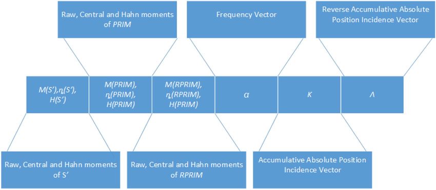
www.nature.com/scientificreports/
to supervise these repairs increasing the risk of developing cancers. Tumor suppressor function of TP53 gene
renders it as cancer driver once mutated. Hence by learning the gene characteristics it is possible to determine
which gene can exhibit cancer driver traits. Genes are the heredity units containing protein-encoding informa-
tion for a specific function. Computational intelligence algorithms are predominantly used for the identification
of obscure patterns within genomic and proteomic data. This study endeavors to identify such patterns from
cancer driver genes and decipher them against passenger genes.
A few major oncogenomic sequencing ventures, such as “The Cancer Genome Atlas” (TCGA)3, the “Inter-
national Cancer Genome Consortium” (ICGC)4, and the “Therapeutically Applicable Research to Generate
Effective Treatments” (TARGET), have made a comprehensive catalog of physical changes overall major can-
cer sorts5,6. Right now, numerous computational strategies have been proposed. Based on their fundamentals,
existing strategies can be partitioned into different categories. The most typical kinds of strategies are based on
transformation recurrence. These strategies discover “significantly mutated genes” (SMG) whose change rates
are altogether higher than the foundation transformation rate and judge them as driver genes. These existing
tools are mainly partitioned into three main categories i.e. frequency-based, sub-network methods, and hotspot-
based methods by their basic rules.
Identification of cancer driver genes plays an important role in precision oncology and personalized cancer
treatment. Scientists working on finding personalized treatment of cancer aims at identifying the genes involved
in the onset of cancer and subsequently taking measures to silence those specific genes or their cancer-causing
functional characteristics. Henceforth, a tool that could accurately and efficiently identify cancer driver genes
is in profound demand. The ability to recognize such driver genes can enable us to disentangle the specific
instrument of disease, and hence play a pivotal role in the advancement of research in novel medications and
treatments for cancer. This study defines an assiduous methodology for a new prediction model for computa-
tional identification of cancer driver genes. The work adapts broadly used approaches in bioinformatics and
computational science for the recognition of cancer driver g enes7–9. A valuable and systematic sequence-based
methodology for an organic framework can be planned by observing the following simple steps (1) development
or determination of a substantial benchmark dataset for training and testing the prediction model; (2) definition
of the organic arrangement tests with a viable numerical expression, reflecting their basic relationship with the
targets concerned; (3) creating an effective computational algorithm for prediction; (4) validation of outcomes
that equitably evaluate the expected precision (5) Providing a framework for public use based upon the carved
out robust model.
Materials and methods
This section contains a detailed description and usage of the computational processes that run the show. The
primary steps are selection/creation of benchmark dataset, test definitions, and extraction of feature vectors that
highlight the attributes of the dataset while the final step is the development and training of a robust prediction
model based on the material gathered within the feature vector as depicted in Fig. 1.
Benchmark dataset collection and its preprocessing. The benchmark dataset usually comprises
experimentally established unambiguous known samples. These samples are further used for training as well as
testing purposes10. The purpose is to develop one high-quality benchmark dataset which is diverse, accurate, and
relevant. Further, the outcome of the experimental work is substantiated through a range of experimental valida-
tion tests like independent set and subsampling (K-fold cross-validation) tests11. Coherent and meaningful data
bears significance since the outcome received is a combination of numerous distinctive unbiased dataset tests.
A meaningful dataset with well-defined annotation of cancer driver gene sequences is gathered. The dataset
is required as a benchmark of authentic cancer driver gene sequences. The benchmark dataset selected for this
study is extracted from the most recent version available on the website namely I ntOgen12. IntOgen lists in all
26,725 cases of mutations in a wide variety of human genes. Most of the cases are passenger mutations that do
not cause cancer while 2901 listed mutations are tumor-causing. A total of 568 cancer driver genes are involved in
these tumors causing mutations. Moreover, 1754 genes involved in passenger mutations were selected exhibiting
the least mutual homology. Subsequently, data gathered in this way is used to formulate a benchmark dataset
for the described problem. The benchmark dataset within the current study is denoted as G, which is defined as
G = G+ UG− (1)
After subtle preprocessing and homology reduction a database was formulated, the final benchmark dataset
contained 568 positive human gene sequences (G+ ) and meticulously selected 1743 negative samples of negative
gene sequences (G− ) obtained from a large collection of passenger genes.
Sample formulation. A DNA sequence can be articulated as
S = ρ1 , ρ2 , ρ3 , . . . , ρi , . . . , ρn (2)
where
(3)
ρ ∈ {A(adenine), C cytosine , G guanine , T thymine }
indicates the nucleotide at any arbitrary position, and ∈ represents an image within the set hypothesis meaning
“member of ”13.
The recent advances in information and data sciences have furnished groundbreaking advances in biotech-
nology. However, one of the most pressing issues in devising such computational models that transform the raw
Scientific Reports | (2021) 11:12281 | https://doi.org/10.1038/s41598-021-91656-8 2
Vol:.(1234567890)
www.nature.com/scientificreports/
Figure 1. Steps towards the construction of a robust prediction model.
data into discrete fixed-sized quantifiable models based upon their grouping information without losing any
grouping physiognomies. Data and features obtained from such designs are instrumental in intelligent target
analysis. Such vector detailings obtained exposure of genomic or proteomic arrangements are best appraised by
machine algorithms (like ‘Neural Networks (CD)’, ‘Random Forest (RF)’ and ‘Support Vector Machine’ (SVM))
which are inherently designed to receive vector input14. It may well be conceivable that in a discrete model all
the sequence-pattern data needs to be transformed into a fixed-size vector without losing crucial information
that determines the properties of the given sequence. To overcome these constraints on sequence-pattern related
data from proteins, the Pseudo Amino Acid Composition (PseAAC)1 was proposed. Later, Chou’s PseAAC15,16
has been deployed in about all of the computational proteomics arenas. Due to its ubiquity and significance in
computational proteomics was incorporated into an efficient computer application called ‘PseAAC-General’17.
Empowered by the triumphs of utilizing PseAAC to bargain with protein/peptide arrangements, its thought
has been amplified to bargain with DNA/RNA arrangements in computational genomics via PseKNC (Pseudo
K-tuple Nucleotide Composition)13. Subsequently, the genomic data is transformed into generalized stable
numerical encoding depicted as R of Eq. (3) as
R = [ζ1 ζ2 ζ3 ζ4 . . . ζu . . . ζ� ] (4)
where ζv (v = 1, 2,…, Ω) is an arbitrary numerical coefficient representing a feature. The components of Eq. (4) are
useful data extricated from the gene sequence. Further, we discuss the methodology used to extract these features.
Statistical moments. For characterizing the components and measurements of Eq. (4) and to have the
quantitative portrayal for cancer driver gene samples of benchmarks dataset we utilize a factual approach. Statis-
Scientific Reports | (2021) 11:12281 | https://doi.org/10.1038/s41598-021-91656-8 3
Vol.:(0123456789)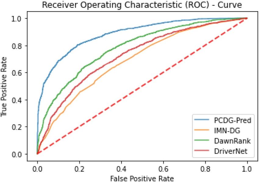
www.nature.com/scientificreports/
tical moments are applied to transform the genomic data into a fixed size. Each moment describes some unique
information that designates the nature of data. Analysts and mathematicians have worked on moments of dif-
ferent distributions18,19. Hahn, raw and central moments of the genomic data are furnished into the feature set
and forms a salient component of an input vector for the predictor. The area and scale of variance incorporated
into the moments act as a tool to decipher among functionally different sequences. Moreover, other moments
that define the asymmetry and the mean of data also help in the construction of a classifier with the appropria-
tion of a labeled dataset. Scientists have observed that the properties of genomic and proteomic sequences are
dependent upon the composition as well as the relative positioning of their bases. Henceforth, for furnishing
the feature vector, only those mathematical and computational models are most apt which are sensitive to the
relative positioning of component nucleotide bases within genomic sequences. It is a critical factor in formulat-
ing yielding and assiduous feature sets18–26. Since Hahn moments require two-dimensional data, therefore, the
genomic sequences are converted into a two-dimensional notation S’ of size k*k which stores the same informa-
tion as S but in a two-dimensional form such that
√
k= n
and
S11 S12 . . . S1n
′ S S . . . S2n
S = 21 22 (5)
: : :
...
Sn1 Sn2 Snn
Further, statistical moments are computed from the obtained square matrix for dimensionality reduction
and forming fixed-size feature vectors27,28. As discussed previously, the three moments deployed in this study
are Hahn, central and raw moments.
Equation 6 describes the operations performed to compute raw moments of order a + b.
n n
Uab = ea f b δef (6)
e=1 f =1
Moments up to order 3 encompass significant information inscribed within the sequences, which are U00,
U01, U10, U11, U20, U02, U21, U12, U03, and U30. Furthermore, to compute the central moments the centroid (x, y)
needs to be computed. The centroid acts as the center of data being visualized. Using this centroid the central
moments are computed as:
n n
b
(e − x)a f − y δef
Vab =
e=1 f =1
(7)
The square grid is used as the discrete input to compute Hahn moments. Hahn moments help describe the
symmetry of data and at the same time, they are reversible. This essentially means that these moments can be
used to reconstruct the original data. The reversibility of moments ensures that the information curtailed within
the original sequences remains intact and is passed forward to the predictor through the corresponding feature
vector. Hahn moments are computed using Eq. (8).
x,y
n (−n)z −p z 2Q + x + y − n − 1 z 1
(−1)z (8)
hn p, Q = (Q + V − 1)n (Q − 1)n ×
z=0 Q + y − 1 z (Q − 1)z z!
Equation (8) makes use of the Pochammer notation which in turn uses the Gamma operator, both these
functions are elaborated by Akmal et al.29,30. Usually, the Hahn coefficient obtained in Eq. (8) is normalized using
the coefficient described in Eq. (9).
G−1 G−1
δpq hpa,b j, Q hqa,b (i, Q), m, n = 0, 1, 2, . . . , Q − 1 (9)
Hpq =
j=0 i=0
Position relative incidence matrix (PRIM). The proposed computational models are furnished for spe-
cific purposes only and are framed within the overall picture for prediction of gene attributes assigning them the
essential grouping as a tool for readily identifying its remarkable traits. There is a clear quantization concern-
ing the precise role of the nucleotide bases. Besides the bases, the position at which each base is placed is very
significant. The position relative incidence matrix31–33 is introduced as an account of the relative positioning of
nucleotide bases regarding each other. The organization of the matrix is given below:
R1→1 R1→2 . . . R1→q . . . R1→M
R2→1 R2→2 . . . R2→q . . . R2→M
: : : :
RPRIM = (10)
Rp→1 Rp→2 . . . Rp→q . . . Rp→M
: : : :
RM→1 RM→2 . . . RM→q . . . RM→M
Scientific Reports | (2021) 11:12281 | https://doi.org/10.1038/s41598-021-91656-8 4
Vol:.(1234567890)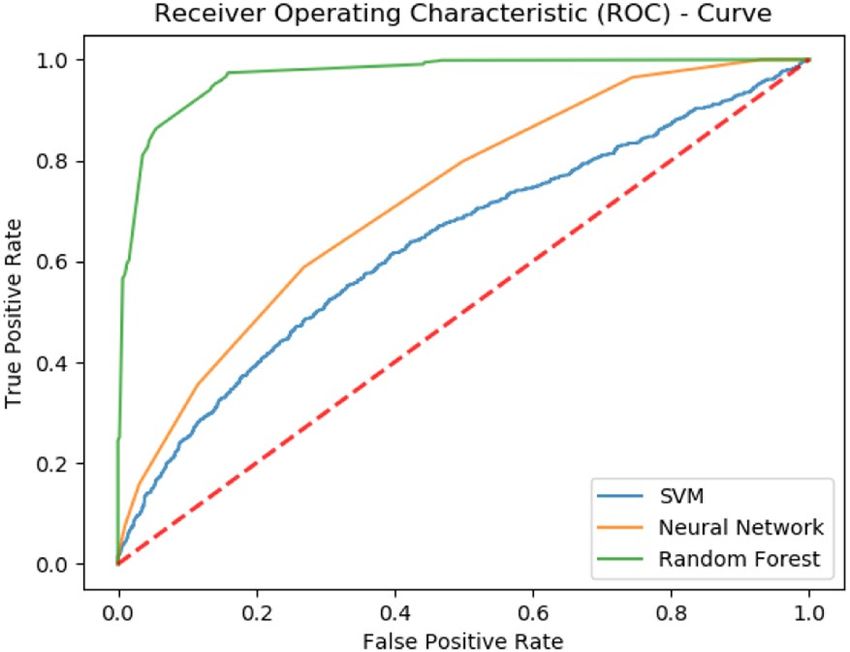
www.nature.com/scientificreports/
In the above matrix, the aggregate of relative places of qth base regarding the first occurrence of pth base is
represented in the component Rp→q . The matrix hence obtained is further used to compute Hahn, central and
raw moments and form coefficients of up to order 3.
Reverse Position Relative Incidence Matrix (RPRIM). The core objective of feature extraction is to
uncover obscure patterns that are embedded within the gene sequences. The gene sequences need to be analyzed
from varying perspectives to sieve out all the information pertinent to its behavior. Experiments show an analy-
sis of the reversed sequence of gene/protein also reveals significant information. The reverse position relative
incidence matrix (RPRIM) is formed based on exactly the described motive. This matrix is derived by reversing
the original sequence and then computing the PRIM for the reversed sequence. An arbitrary element on RPRIM
say Ri→j hold information regarding the relative positioning of the ith nucleotide base relative to the jth nucleo-
tide base within the reverse sequence. The RPRIM matrix is represented as
R1→1 R1→2 . . . R1→q . . . R1→M
R2→1 R2→2 . . . R2→q . . . R2→M
: : : :
RRPRIM = (11)
R
p→1 p→2 R . . . R p→q . . . R
p→M
: : : :
RM→1 RM→2 . . . RM→q . . . RM→M
Further for uniformity, the Hahn, raw, and central moments are also computed.
Frequency vector determination. The sequence order, as well as the composition of a nucleotide chain,
impart their effect in exhibiting the overall attributes of a gene. Previously, the PRIM and RPRIM matrices we
discussed, both these matrices help to extract the sequence-related correlations of the nucleotide bases. The
frequency vector (FV) summarizes the composition-related information of a gene. Each element of this vector
provides the count of the occurrence of the nucleotide within the gene sequence. The vector is represented as
α = {ε1 , ε2 , . . . , εn } (12)
where εi provides the count of the overall occurrence of the ith nucleotide base.
Accumulative absolute position incidence vector (AAPIV) generation. A feature extraction
model that is capable of extracting all the aspects relevant to the sequence ordering and composition of the gene
sequence. The FV provides information regarding the frequency of occurrence of each nucleotide base, similarly,
the accumulative absolute position incidence vector provides the cumulative information regarding the position
occurrence for each specific nucleotide base. It is represented as
K = { 1 , 2 , . . . n } (13)
where the ith component of AAPIV is computed as
n
i =
k=1
βk (14)
and βk is an arbitrary position of occurrence for a specific nucleotide. An arbitrary element i of AAPIV will
contain the sum of all the positions of occurrence of the ith nucleotide.
Reverse accumulative absolute position incidence vector (RAAPIV) generation. A deeper per-
spective regarding the hidden patterns within the gene sequence is provided by the reverse sequence. Computa-
tion of AAPIV for the reverse sequence of the gene is termed RAAPIV. It is represented as:
= {n1 , n2 , . . . , nm } (15)
An arbitrary element ni of RAAPIV will contain the sum of all the positions of occurrence of the i nucleotide
th
within the reverse sequence.
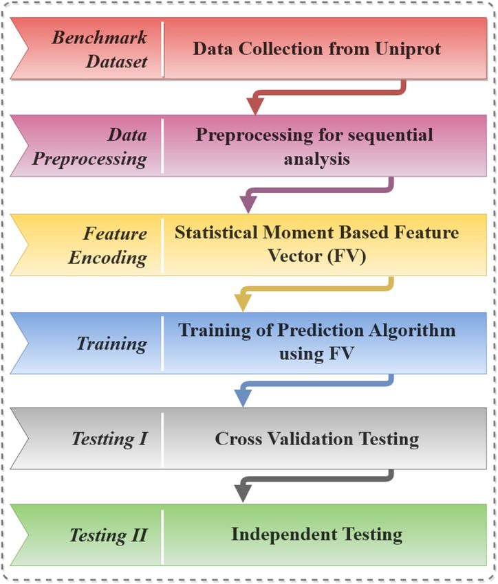
Feature vector formulation. Each primary sequence is transformed into a fixed scale notation of Eq. (4).
Moments are computed Large matrices G’, PRIM, and RPRIM are transformed into succinct form by computing
raw, central, and Hahn moments. Subsequently, these moments are assimilated into a feature vector along with
FV, AAPIV, and RAAPIV. Figure 2. shows the structure of a feature vector illustrating each component. Coef-
ficients contained in this feature vector corresponding to a primary sequence of arbitrary length. A comprehen-
sive set of feature vectors is computed for all the samples in the dataset.
Random forest. Random forests or random decision forests are an ensemble learning method for classifi-
cation, regression, and other tasks that are performed by constructing a multitude of decision trees at training
time. The overall output of the class is represented as the mode or mean of all the individual trees34,35. Figure 3
shows the architecture of the Random forest tree used for the purpose.
Artificial neural network. Artificial neural networks are a structure of linked neurons in which the output
of the previous neuron in one layer is connected to the input of a neuron in the next layer. The activation func-
Scientific Reports | (2021) 11:12281 | https://doi.org/10.1038/s41598-021-91656-8 5
Vol.:(0123456789)www.nature.com/scientificreports/
Figure 2. Depicts the structure of a feature vector.
Figure 3. The architecture of random forest classifier for the proposed prediction model.
tion at each neuron uses the inputs from each neuron in the previous layer and their assigned weights to provide
an output. The weights of neurons are adjusted iteratively until the objective function is a chieved24,25,34–36. The
architecture of the neural network used is described in Fig. 4.
Scientific Reports | (2021) 11:12281 | https://doi.org/10.1038/s41598-021-91656-8 6
Vol:.(1234567890)www.nature.com/scientificreports/
Figure 4. The architecture of the artificial neural network classifier for the proposed prediction model.
Figure 5. Architecture of SVM Classifier for the proposed prediction model.
Support vector machine. Support-vector machines are supervised learning models with associated learn-
ing algorithms that analyze data used for classification and regression analysis. SVMs are commonly used in
classification problems and as such. SVMs are based on the idea of finding a hyperactive plane, as depicted in
Fig. 5 that best divides the dataset into two classes.
Support vectors are the data points nearest to the hyperplane, the points of a data set that, if removed, would
alter the position of the dividing hyperplane. Hence, they are considered critical elements of a data set37–39.
Supervised learning models are those which require that the data is already annotated or labeled. On the
other hand, unsupervised learning models use unlabeled data and they try to make sense of data as they learn
patterns within it. Usually, classification problems in proteomics and genomics using experimentally obtained
data regarding a specific phenomenon. Several proteomic and genomic databases are available which work as a
repository of previous experimental findings. Known and well-annotated data is curated from such repositories.
Hence, supervised learning models are the natural choice for classifiers using such data. Discussed supervised
learning models are facilitated by combining all the feature vectors such that each row corresponds to a single
primary sequence sample to form an input array. Since the data is experimentally collected and well-annotated,
an expected output matrix is also furnished to facilitate supervised learning. Further, both these matrices are
used to train the described classifiers. The input array is used as training data by these models while the expected
outputs are used to calculate errors throughout the learning process of each model.
Scientific Reports | (2021) 11:12281 | https://doi.org/10.1038/s41598-021-91656-8 7
Vol.:(0123456789)www.nature.com/scientificreports/
Accuracy metrics
Method Sn (%) Sp (%) Acc (%) MCC (%)
PCDG-RF 88.10 92.26 91.08 0.7867
PCGD-SVM 50.16 72.14 69.45 0.1585
PCGD-NN 64.71 77.75 75.19 0.3660
Table 1. Self-consistency experimental results for PCDG-Pred.
Results and discussions
The estimation of the performance of the predictor in terms of accuracy is very important to ensure that the
right kind of assessment for the prediction algorithm. To establish these facts researchers have developed sev-
eral quantitative metrics. These metrics are established based on well-defined experimental tests and hence be
confidently used as a comparative parameter among competitive models.
Accuracy metrics. Four interlinked quantitative metrics are generally used to assess the performance of a
predictor. The accuracy metric is denoted as Acc, it provides an overall picture of the prediction accuracy of the
model. The second metric is named sensitivity denoted as (Sn), which represents the capability of the model in
accurately predicting positive samples. Similarly, the specificity denoted as ( Sp) is used to provide a quantitative
measure for the accuracy of the model in predicting negative samples40. Lastly, Mathew’s correlation coefficient
factor denoted as (MCC) is a stable measure for the accuracy of the predictor when the number of positive and
negative samples is unbalanced.
For simplicity and readability, a formulation for these metrics introduced by W. Chen, Feng, & Lin in 2 01341
is illustrated. The authors represented these metrics formulation expressions in such a way that they are more
readable and easier to implement.
P±
Sp = 1 − 0 ≤ Sp ≤ 1 (16)
P−
P∓
Sn = 1 − 0 ≤ Sn ≤ 1 (17)
P+
+ −
P− + P+
Acc = 1 − 0 ≤ Acc ≤ 1 (18)
P+ + P−
P± ∓
1− + PP −
P+
MCC =
(19)
∓ ± P ± −P ∓
1 + P P−P
+ 1+ P−
where P + represents the actual number of cancer driver genes, P− +
is the number of cancer driver genes predicted
as passenger genes, P is the actual number of passenger genes in the test while P+
− −
is the number of passenger
genes predicted as cancer driver genes. The above equations signify that the sensitivity Sn will be maximum
when no sample is wrongly predicted as a passenger gene i.e. P− +
= 0, similarly, the sensitivity Sp is maximum
when P+ −
= 0. The overall picture of the predictor performance is portrayed by Acc and MCC. The prediction
model is most accurate if Acc = 1 and also MCC = 1 which essentially means that no sample has been wrongfully
predicted i.e. N−+
= N+ −
= 0. There are some other changes as well in which it is possible that no solitary cancer
driver gene gives you the positive dataset and all the non-cancer driver genes give you the negative dataset and
show that the figures are dishonestly anticipated by the researchers. In the case of the other extreme, MCC value
will be − 1 and the value of Acc will be 0. In the case of a binary predictor, there are only two classes and the
probability of predicting correctly is 50%. An accuracy of 50% is considered as a benchmark, any predictor to
be acceptable must at least have an accuracy better than 50 percent. For such a predictor the value of MCC will
be 0 and the value of Acc will be 0.5 where N+ −
= N − /2 and N− +
= N + /2, which essentially implies that only
half of the cancer genes and half of the passenger genes will be predicted accurately. The use of these metrics
brings acceptability and acclaim to the experimental results established by the study. Furthermore, these metrics
can also be expanded for multiclass predictors7,42–44. The performance of a predictor is substantiated through a
set of well-defined tests. These tests yield accuracy metrics which firstly signify quantitatively how well a model
performs and secondly, establishes the suitability of the model even if new data is not readily available.
Self‑consistency validation. The self-consistency test is one of the most basic tests and is generally used
to establish the appropriateness of the predictor. Previously, a set of feature vectors constituting positive and
negative samples was collected and used for training. After sufficient training of the model, it is validated using
a self-consistency test. This test reverberates that the predictor is tested with the same samples which were used
to train it. Henceforth, all the classifiers trained on the benchmark dataset are tested. The number of samples
correctly predicted by each of the classifiers is tabulated to calculate the accuracy metrics as shown in Table 1.
Scientific Reports | (2021) 11:12281 | https://doi.org/10.1038/s41598-021-91656-8 8
Vol:.(1234567890)www.nature.com/scientificreports/
Figure 6. Self-consistency ROC curves for PCDG-Pred.
Accuracy metrics
Method Sn (%) Sp (%) Acc (%) MCC (%)
PCDG-RF 91.06 81.27 87.26 0.6482
PCGD-SVM 48.21 68.11 65.42 0.412
PCGD-NN 61.67 74.36 71.87 0.331
Table 2. Independent testing results for PCDG-RF.
Consequently, a receiver operating characteristic (ROC) curve shows a comparison of accuracy exhibited by
each predictor. It can be noticed that the performance of the Random Forest-based predictor is fairly thriving as
compared to SVM and neural network-based predictor. In Fig. 6, it is noticed that the area under the curve of
the RF-based predictor is maximum.
All the results yielded by the described test are shown in Table 1 and Fig. 1, as illustrated. It shows that the
predicted rule which was performed during the study was similar to the original proposed computational method
of the study. It also shows the normal execution of all the proposed frameworks which are concerned with this
research and the study.
Independent set testing. Independent set testing is the most trivial test for gauging the functioning con-
duct of the predictor for unknown data. Usually, to perform this test the data is partitioned into two unequal-
sized partitions. The larger partition is used to train the predictor and the smaller one is used to test its accuracy.
Since numerous permutations exist for making such partitions, the test is repeated several times to ascertain its
accuracy. The extracted benchmark dataset is used to perform this test. A partition spanning over 70% of the
dataset was used to train the predictors, while the rest of the 30% was left for testing. The test was repeated 10
times with different partitions. The average accuracy metrics obtained from each predictor are listed in Table 2.
Again, the test shows that the RF-based predictor outperforms the accuracy of SVM and neural network-based
predictors. The comparison of all the machine learning models is shown in the ROC graph in Fig. 7.
Cross‑validation. The self-consistency test provides some feedback regarding the comparative perfor-
mance of different models. However, it does not reflect the capability of the model to work on unknown data.
Independent data set testing does provide a notion regarding the capability of the model to work on unknown
data. Although, independent set testing is performed on randomly partitioned data still there is still a possibility
that a major troublesome portion of data is left out of this test. A more rigorous test that alleviates this situation
is the cross-validation test. Cross-validation is a rigorous test that spans over all the s amples32,33,42,45. The dataset
is partitioned into k disjoint folds. The test will be repeated k times. Each time the testing is performed on a
different partition while the rest of the k-1 partitions are used for training. In the end, the results reported from
each test carried out k-times are averaged to compute the overall prediction accuracy. This strategy proves most
beneficial when new test data is not readily available. The cross-validation test provides a fair picture regarding
the overall performance of the predictor on unknown data as no data item is left out of the testing process. The
cross-validation is a rigorous test as it spans over all the datasets and every item of the dataset has to be tested
on the prediction model. tenfold cross-validation is performed on all the predictors. The data is divided into 10
disjoint sets such that their composition forms the whole data. Items within each dataset are placed by randomly
selecting them from the combined dataset. Each fold is tested on predictors furnished through training of the
rest of the folds. The average accuracy metrics obtained from testing of all 10 folds are reported in Table 3 for all
the predictors.
Scientific Reports | (2021) 11:12281 | https://doi.org/10.1038/s41598-021-91656-8 9
Vol.:(0123456789)www.nature.com/scientificreports/
Figure 7. Independent Set testing for PCDG-RF.
Accuracy metrics
Method Sn (%) Sp (%) Acc (%) MCC (%)
PCDG-RF 84.12 96.12 92.48 0.8141
PCGD-SVM 71.66 99.54 86.81 0.552
PCGD-NN 81.39 83.01 88.23 0.601
Table 3. Tenfold cross-validation results for PCDG-Pred.
Figure 8. 10-Fold cross-validation for all predictors.
Subsequently, Fig. 8 shows a ROC curve depicting the performance of the most optimal PCDG-RF predictor.
This test also establishes that the RF-based algorithm provides greater yield as compared to SVM and neural
network.
Randomly curated cancer driver samples over numerous iterations were tested on PCDG-Pred along with
other existing cancer driver gene predictors namely D awnRank46, DriverNet47, and IMN-DG48. The DawnRank
algorithm ranks a gene based on the disruption it causes resulting in downstream genes. DriverNet studies the
disruptions caused in transcriptional patterns due to genomic aberrations leading to cancer. Integrative Module-
Based Cancer Driver (IMN-DG) prediction methodology proposes machine learning techniques for the identi-
fication of cancer driver genes. The comparison of these techniques is illustrated in ROC curves (Fig. 9) plotted
using the mean of True Positive Rate (TPR) and False Positive Rate (FPR) for all the iterations.
The graph shows that the proposed technique outperforms the previous technique as it shows the greatest
area under the curve (AUC) of 0.84 for the curated datasets.
Scientific Reports | (2021) 11:12281 | https://doi.org/10.1038/s41598-021-91656-8 10
Vol:.(1234567890)www.nature.com/scientificreports/
Figure 9. Shows ROC curve depicting the performance of proposed predictor along with existing predictors.
The area under the curve (AUC = 0.84) for the proposed technique promises the best performance.
Identification of cancer driver genes is an important aspect of precision and personalized oncology. Bioinfor-
matics tools that could accurately and readily analyze sequencing data in this respect have insightful demand.
The proposed model is systematically organized by accumulating robust data, applying meaningful feature
extraction techniques, and then using state of art machine learning algorithms for training. Further, the model
is rigorously tested and validated using different validation techniques. Test results exhibit that the PCDG-RF
has the best accuracy of 91.08%, 87.26%, and 92.48% for self-consistency, independent set testing, and tenfold
cross-validation respectively. The other algorithms were unable to match PCDG-RF which yielded an accuracy
for tenfold cross-validation of 86.81% and 88.23% for PCDG-SVM and PCDG-NN respectively. Further, to
ascertain the robustness of the proposed model, its accuracy was tested against other existing models for the
identification of cancer drivers. A randomly selected set of cancer driver genes was iteratively tested with the
proposed model along with existing models such as DawnRank, DriverNet, and IMN-DG. Results hence obtained
are illustrated by plotting a receiver operating characteristics graph using the true positive rate and false-positive
rate. The proposed model performs significantly better as compared with existing models with an area under
the curve of 0.84 while others seem to cover a lesser area as illustrated in Fig. 9. Based on these findings it can
be confidently concluded that the proposed model can be used as a robust tool for the identification of cancer
driver genes while playing an important role as a bioinformatics tool in cancer research.
Web server. The significance of a web server application is thoroughly realized by the fact that it has all the
abilities to provide an easy-to-understand computational analysis promptly. This need is felt by leading research-
ers working in a specific domain. Researchers working on such studies try to make sure that the webserver is
freely available to help any future developments and advancements relevant to the study. Furthermore, the whole
picture implies the fact that the fundamentals of computational science have improved in the last few years espe-
cially those relevant to data science and c lassification31. This further strengthens the notion that computational
applications assisting medical science are going for an u pheaval32 shortly. For all these reasons several efforts
are made to make sure that a web server is developed for all the prediction techniques used these days. Thus, a
web-based implementation of the methodology has been made available at https://pcdg-pred.herokuapp.com.
Conclusion
Oncology is recognized as a highly prioritized area of research. Science and research have uncovered substantial
myths regarding cancer by identifying well-defined targets to investigate and mediate improvements in this area.
Researchers have established that cancer is a genetic disorder. Cancer is driven by distinctive changes and basic
variations in a genetic structure called mutations. In case a gene mutation results in uncontrollable growth of
cancer then the gene is called the cancer driver gene otherwise, if the mutation does not cause cancer then it’s
called a passenger mutation. Cancer is one of the most preeminent disorders whose progression has nefarious
effects on human life and may eventually lead to death. Recognition of cancer driver genes is a basic instru-
ment of oncological studies. Numerous methods exist for the identification of oncological genetic progression
through mutation if provided with years old original sequence along with the current mutated one. Researchers
are actively working to provide personalized treatment for this life-threatening disorder. Gene silencing is a key
area being inquired by researchers that could help silence specific cancer driver genes. The proposed bioinformat-
ics tool can greatly facilitate researchers and the medical community in this aspect by identification of specific
cancer driver gene sequencing obtained through next-generation sequencing of patient DNA. This paper uses
different techniques and devices a feature extraction technique based on the relative positioning of nucleotide
bases. Subsequently, for dimensionality reduction, statistical moments are employed to form a fixed-sized feature
vector for each gene sequence. The most recent set up to date data regarding cancer drivers and passenger genes
is extracted from IntOgen site. The feature set formed is used as input for the training of the various classifiers.
Experimental results show that the most suitable and accurate classifier for deciphering obscure patterns among
cancer driver genes is random forest. Hence, a combination of devised feature sets and random forest forms a
Scientific Reports | (2021) 11:12281 | https://doi.org/10.1038/s41598-021-91656-8 11
Vol.:(0123456789)www.nature.com/scientificreports/
comprehensive platform for the identification of cancer driver genes. The best accuracy achieved for the tenfold
cross-validation test is 92.48%. The present study can indeed aid in the emerging personalized treatment of cancer
through the identification of specific cancer-causing genes using DNA sequencing of the patient.
Received: 6 January 2021; Accepted: 19 May 2021
References
1. Xu, Y., Ding, J., Wu, L.-Y. & Chou, K.-C. iSNO-PseAAC: Predict cysteine S-nitrosylation sites in proteins by incorporating position
specific amino acid propensity into pseudo amino acid composition. PLoS ONE 8, e55844 (2013).
2. Dietlein, F. et al. Identification of cancer driver genes based on nucleotide context. Nat. Genet. 52, 208–218 (2020).
3. Network, C. G. A. R. Comprehensive genomic characterization defines human glioblastoma genes and core pathways. Nature 455,
1061 (2008).
4. Lathrop, M. et al. International Network of Cancer Genome Projects (The International Cancer Genome Consortium, 2010).
5. Korthauer, K. D. & Kendziorski, C. MADGiC: A model-based approach for identifying driver genes in cancer. Bioinformatics 31,
1526–1535 (2015).
6. Kumar, R. D., Swamidass, S. J. & Bose, R. Unsupervised detection of cancer driver mutations with parsimony-guided learning.
Nat. Genet. 48, 1288 (2016).
7. Chou, K.-C. Some remarks on predicting multi-label attributes in molecular biosystems. Mol. BioSyst. 9, 1092–1100 (2013).
8. Liu, B., Long, R. & Chou, K.-C. iDHS-EL: Identifying DNase I hypersensitive sites by fusing three different modes of pseudo
nucleotide composition into an ensemble learning framework. Bioinformatics 32, 2411–2418 (2016).
9. Zhang, C.-J. et al. iOri-Human: Identify human origin of replication by incorporating dinucleotide physicochemical properties
into pseudo nucleotide composition. Oncotarget 7, 69783 (2016).
10. Feng, P. et al. iRNA-PseColl: Identifying the occurrence sites of different RNA modifications by incorporating collective effects of
nucleotides into PseKNC. Mol. Ther.-Nucleic Acids 7, 155–163 (2017).
11. Guo, S.-H. et al. iNuc-PseKNC: A sequence-based predictor for predicting nucleosome positioning in genomes with pseudo k-tuple
nucleotide composition. Bioinformatics 30, 1522–1529 (2014).
12. Gonzalez-Perez, A. et al. IntOGen-mutations identifies cancer drivers across tumor types. Nat. Methods 10, 1081–1082 (2013).
13. Feng, P. et al. iDNA6mA-PseKNC: Identifying DNA N6-methyladenosine sites by incorporating nucleotide physicochemical
properties into PseKNC. Genomics 111, 96–102 (2019).
14. Hussain, W., Khan, Y. D., Rasool, N., Khan, S. A. & Chou, K.-C. SPrenylC-PseAAC: A sequence-based model developed via Chou’s
5-steps rule and general PseAAC for identifying S-prenylation sites in proteins. J. Theor. Biol. 468, 1–11 (2019).
15. Cao, D.-S., Xu, Q.-S. & Liang, Y.-Z. propy: A tool to generate various modes of Chou’s PseAAC. Bioinformatics 29, 960–962 (2013).
16. Lin, S. and Lapointe, J., Theoretical and experimental biology in one —A symposium in honour of Professor Kuo-Chen Chou’s
50th anniversary and Professor Richard Giegé’s 40th anniversary of their scientific careers. Journal of Biomedical Science and
Engineering, 6, 435–442, https://doi.org/10.4236/jbise.2013.64054(2013).
17. Chou, K. C. Prediction of protein cellular attributes using pseudo-amino acid composition. Proteins Struct. Funct. Bioinform. 43,
246–255 (2001).
18. Khan, Y. D., Ahmed, F. & Khan, S. A. Situation recognition using image moments and recurrent neural networks. Neural Comput.
Appl. 24, 1519–1529 (2014).
19 Khan, Y. D., Khan, S. A., Ahmad, F. & Islam, S. Iris recognition using image moments and k-means algorithm. Sci. World J. 2014,
1–9 (2014).
20 Butt, A. H. & Khan, Y. D. Prediction of S-sulfenylation sites using statistical moments based features via CHOU’S 5-step rule. Int.
J. Pept. Res. Ther. 26, 1–11 (2019).
21. Butt, A. H. & Khan, Y. D. CanLect-Pred: A cancer therapeutics tool for prediction of target cancerlectins using experiential anno-
tated proteomic sequences. IEEE Access 8, 9520–9531 (2019).
22. Butt, A. H., Rasool, N. & Khan, Y. D. Predicting membrane proteins and their types by extracting various sequence features into
Chou’s general PseAAC. Mol. Biol. Rep. 45, 2295–2306 (2018).
23. Butt, A. H., Rasool, N. & Khan, Y. D. Prediction of antioxidant proteins by incorporating statistical moments based features into
Chou’s PseAAC. J. Theor. Biol. 473, 1–8 (2019).
24. Khan, Y. D., Rasool, N., Hussain, W., Khan, S. A. & Chou, K.-C. iPhosT-PseAAC: Identify phosphothreonine sites by incorporating
sequence statistical moments into PseAAC. Anal. Biochem. 550, 109–116 (2018).
25. Khan, Y. D., Rasool, N., Hussain, W., Khan, S. A. & Chou, K.-C. iPhosY-PseAAC: Identify phosphotyrosine sites by incorporating
sequence statistical moments into PseAAC. Mol. Biol. Rep. 45, 2501–2509 (2018).
26. Rehman, K. U. U. & Khan, Y. D. A scale and rotation invariant urdu nastalique ligature recognition using cascade forward back-
propagation neural network. IEEE Access 7, 120648–120669 (2019).
27. Akbar, S. & Hayat, M. iMethyl-STTNC: Identification of N6-methyladenosine sites by extending the idea of SAAC into Chou’s
PseAAC to formulate RNA sequences. J. Theor. Biol. 455, 205–211 (2018).
28. Ilyas, S. et al. iMethylK-PseAAC: Improving accuracy of lysine methylation sites identification by incorporating statistical moments
and position relative features into general PseAAC via Chou’s 5-steps rule. Curr. Genomics 20, 275–292 (2019).
29. Akmal, M. A. et al. Using Chou’s 5-steps rule to predict O-linked serine glycosylation sites by blending position relative features
and statistical moment. IEEE/ACM Trans. Comput. Biol. Bioinform. 12, 12. https://doi.org/10.1109/TCBB.2020.2968441 (2020).
30 Akmal, M. A., Rasool, N. & Khan, Y. D. Prediction of N-linked glycosylation sites using position relative features and statistical
moments. PLoS ONE 12, e0181966 (2017).
31. Awais, M. et al. iPhosH-PseAAC: Identify phosphohistidine sites in proteins by blending statistical moments and position rela-
tive features according to the Chou’s 5-step rule and general pseudo amino acid composition. IEEE/ACM Trans. Comput. Biol.
Bioinform. 18, 596–610 (2019).
32. Barukab, O., Khan, Y. D., Khan, S. A. & Chou, K.-C. iSulfoTyr-PseAAC: Identify tyrosine sulfation sites by incorporating statistical
moments via Chou’s 5-steps rule and pseudo components. Curr. Genomics 20, 306–320 (2019).
33. Khan, S. A., Khan, Y. D., Ahmad, S. & Allehaibi, K. H. N-MyristoylG-PseAAC: Sequence-based prediction of N-myristoyl glycine
sites in proteins by integration of PseAAC and statistical moments. Lett. Org. Chem. 16, 226–234 (2019).
34. Biau, G. & Scornet, E. A random forest guided tour. TEST 25, 197–227 (2016).
35. Taherzadeh, G., Zhou, Y., Liew, A. W. C., & Yang, Y., Structure-based prediction of protein–peptide binding regions using Random
Forest. Bioinformatics, 34(3), 477–484, (2018).
36. Khan, Y. D., Batool, A., Rasool, N., Khan, S. A. & Chou, K.-C. Prediction of nitrosocysteine sites using position and composition
variant features. Lett. Org. Chem. 16, 283–293 (2019).
37 Huang, M.-W., Chen, C.-W., Lin, W.-C., Ke, S.-W. & Tsai, C.-F. SVM and SVM ensembles in breast cancer prediction. PLoS ONE
12, e0161501 (2017).
Scientific Reports | (2021) 11:12281 | https://doi.org/10.1038/s41598-021-91656-8 12
Vol:.(1234567890)www.nature.com/scientificreports/
38. Vapnik, V. & Izmailov, R. Knowledge transfer in SVM and neural networks. Ann. Math. Artif. Intell. 81, 3–19 (2017).
39 Suthaharan, S. Machine Learning Models and Algorithms for Big Data Classification 207–235 (Springer, 2016).
40. Chen, J., Liu, H., Yang, J. & Chou, K.-C. Prediction of linear B-cell epitopes using amino acid pair antigenicity scale. Amino Acids
33, 423–428 (2007).
41. Chen, W., Feng, P.-M., Lin, H. & Chou, K.-C. iRSpot-PseDNC: Identify recombination spots with pseudo dinucleotide composi-
tion. Nucleic Acids Res. 41, e68–e68 (2013).
42. Khan, Y. D. et al. iProtease-PseAAC (2L): A two-layer predictor for identifying proteases and their types using Chou’s 5-step-rule
and general PseAAC. Anal. Biochem. 588, 113477 (2020).
43. Song, J. et al. PREvaIL, an integrative approach for inferring catalytic residues using sequence, structural, and network features in
a machine-learning framework. J. Theor. Biol. 443, 125–137 (2018).
44. Song, J. et al. iProt-Sub: A comprehensive package for accurately mapping and predicting protease-specific substrates and cleavage
sites. Brief Bioinform. 20, 638–658 (2019).
45. Ehsan, A. et al. iHyd-PseAAC (EPSV): Identifying hydroxylation sites in proteins by extracting enhanced position and sequence
variant feature via chou’s 5-step rule and general pseudo amino acid composition. Curr. Genomics 20, 124–133 (2019).
46. Hou, J. P. & Ma, J. DawnRank: Discovering personalized driver genes in cancer. Genome Med. 6, 1–16 (2014).
47. Bashashati, A. et al. DriverNet: Uncovering the impact of somatic driver mutations on transcriptional networks in cancer. Genome
Biol. 13, 1–14 (2012).
48. Lu, X. et al. The integrative method based on the module-network for identifying driver genes in cancer subtypes. Molecules 23,
183 (2018).
Acknowledgements
This project was funded by the Deanship of Scientific Research (DSR), King Abdulaziz University, Jeddah,
under Grant No. (DF-668-611-1441). The authors, therefore, gratefully acknowledge DSR technical and financial
support.
Author contributions
Y.K. conceptualized the work and formulated methodology to yield results, S.M. worked on data acquisition
and supervised the overall work.
Competing interests
The authors declare no competing interests.
Additional information
Supplementary Information The online version contains supplementary material available at https://doi.org/
10.1038/s41598-021-91656-8.
Correspondence and requests for materials should be addressed to Y.D.K.
Reprints and permissions information is available at www.nature.com/reprints.
Publisher’s note Springer Nature remains neutral with regard to jurisdictional claims in published maps and
institutional affiliations.
Open Access This article is licensed under a Creative Commons Attribution 4.0 International
License, which permits use, sharing, adaptation, distribution and reproduction in any medium or
format, as long as you give appropriate credit to the original author(s) and the source, provide a link to the
Creative Commons licence, and indicate if changes were made. The images or other third party material in this
article are included in the article’s Creative Commons licence, unless indicated otherwise in a credit line to the
material. If material is not included in the article’s Creative Commons licence and your intended use is not
permitted by statutory regulation or exceeds the permitted use, you will need to obtain permission directly from
the copyright holder. To view a copy of this licence, visit http://creativecommons.org/licenses/by/4.0/.
© The Author(s) 2021
Scientific Reports | (2021) 11:12281 | https://doi.org/10.1038/s41598-021-91656-8 13
Vol.:(0123456789)You can also read