Domain Decomposition in Computational Homogenization with Million-way Parallelism - Axel Klawonn, Stephan Köhler, Martin Lanser, and Oliver Rheinbach
←
→
Page content transcription
If your browser does not render page correctly, please read the page content below
Axel Klawonn, Stephan Köhler, Martin Lanser,
and Oliver Rheinbach

Domain Decomposition in
Computational Homogenization with
Million-way Parallelism

PREPRINT 2018-06
Fakultät für Mathematik und Informatik

ISSN 2512-3750
Axel Klawonn, Stephan Köhler,
      Martin Lanser, and Oliver Rheinbach

Domain Decomposition in Computational Homogenization
            with Million-way Parallelism

                   TU Bergakademie Freiberg

                   Fakultät für Mathematik und Informatik
                   Prüferstraße 9

                   09599 FREIBERG
                   http://tu-freiberg.de/fakult1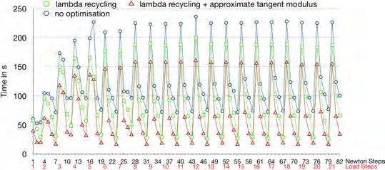
ISSN 1433 – 9307
Herausgeber:       Dekan der Fakultät für Mathematik und Informatik

Herstellung:       Medienzentrum der TU Bergakademie Freiberg
DOMAIN DECOMPOSITION IN COMPUTATIONAL
      HOMOGENIZATION WITH MILLION-WAY PARALLELISM∗
       AXEL KLAWONN† , STEPHAN KÖHLER‡ , MARTIN LANSER† , AND OLIVER
                                           RHEINBACH‡
                                          April 25, 2018
    Abstract. Computational homogenization using the well-known FE2 approach combined with
fast domain decomposition and algebraic multigrid solvers is described. The methods are collected in
the software package FE2TI. A focus is on highly parallel scalability to enable detailed micro-macro
simulations on today’s supercomputers and on those of the upcoming exascale era. Numerical re-
sults using our FE2TI software are presented considering different grids on both, the macroscopic and
microscopic level. Unstructured as well as structured grids with different irregular domain decom-
positions are considered on the microscale. Several optimizations of the core domain decomposition
solvers for nonlinear problems, i.e., Newton-Krylov-FETI-DP and Nonlinear-FETI-DP, are investi-
gated and the performance of the FE2TI package is improved by more than a factor of two using
relatively elementary techniques. Finally, weak scaling results from a few nodes up to a million
parallel processes are presented.

   Key words. homogenization, multiphase steel, computational homogenization, FE2 method,
FETI-DP, domain decomposition, nonlinear domain decomposition, elasto-plasticity,

   AMS subject classifications. 68W10, 68U20, 65N55, 65F08, 65Y05, 74Q05

    1. Introduction. In this paper, we present algorithms and software for the di-
rect computational homogenization of micro-heterogeneous media in nonlinear struc-
tural mechanics. Our approach is based on the combination of an MPI-parallel imple-
mentation of the well-known FE2 computational homogenization method with efficient
MPI-parallel iterative solvers, e.g., from domain decomposition (DD) and algebraic
multigrid, for the problems on the micro- as well as on the macroscale. An earlier
version of our software has already been demonstrated to be applicable to problems
in the simulation of dual-phase steel [36, 34]. The improved software is able to lever-
age the largest supercomputers available for the computational homogenization of
micro-heterogeneous materials using million-way concurrency and beyond.
    It is our goal, to pave the way for predictive simulations in virtual material testing,
with a focus on modern multiphase steels as a show-case, through robust and scal-
able computational algorithms, optimized software, and advanced modeling; see [50]
for a discussion of mathematics-based advanced computing as a means of discovery
and innovation. Our project EXASTEEL is part of the German exascale initiative
SPPEXA1 (Software for Exascale Computing) to develop algorithms and software for
the next generation of supercomputers of the exascale era with parallelism beyond
107 parallel processes or threads.
    The FE2 method is a computational micro-macro homogenization approach which
incorporates micromechanical finite element simulations into macroscopic finite ele-
   ∗ This work was supported in part by Deutsche Forschungsgemeinschaft (DFG) through the Pri-

ority Programme 1648 ”Software for Exascale Computing” (SPPEXA) under grants KL 2094/4-1,
KL 2094/4-2, RH 122/2-1, and RH 122/3-2.
    † Mathematisches Institut, Universität zu Köln, Weyertal 86-90, 50931 Köln, Germany,

axel.klawonn@uni-koeln.de, martin.lanser@uni-koeln.de, url: http://www.numerik.uni-koeln.de
    ‡ Institut für Numerische Mathematik und Optimierung, Fakultät für Mathematik und

Informatik, Technische Universität Bergakademie Freiberg, Akademiestr. 6, 09596 Freiberg,
oliver.rheinbach@math.tu-freiberg.de, stephan.koehler@math.tu-freiberg.de, url:    http://www.
mathe.tu-freiberg.de/nmo/mitarbeiter/oliver-rheinbach
     1 http://www.sppexa.de

                                                 1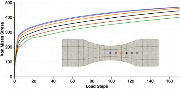
2            A. KLAWONN, S. KÖHLER, M. LANSER, AND O. RHEINBACH

ment simulations. It is well established in the engineering community for many years;
see, e.g., [58, 23, 47, 56, 44, 24, 25, 57],
     In this approach, at each Gauß integration point of the macroscopic finite element
problem a microscopic finite element problem, defined on a representative volume
element (RVE), is attached. The meshes for the finite element simulations on the
RVEs are chosen such that they are able to resolve the micro-heterogeneities. The
computational micro-macro approach replaces a phenomenological material law on
the macroscale; see [57] for an introduction to the FE2 method. Computational
homogenization approaches such as the FE2 method rely on the assumption of scale
separation, i.e., the features of the microstructure are assumed to be magnitudes
smaller than the diameter of the macroscopic finite elements. However, detailed micro-
macro simulations using the FE2 method were still out of reach until recently when
supercomputers with million-way concurrency became available.
     For certain materials the discretization of the macroscopic mechanical part down
to its microstructure may become feasible as the computational power grows towards
the exascale era. Such approaches are then also sometimes referred to as direct numer-
ical simulations in solid mechanics [10, 9]. Note that in [10, 9] a voxel approximation
(using hexahedral finite elements) of the grain structure is used in order to avoid
difficulties in the construction of reliable meshes for realistic grain structures.
     In the present paper, to avoid this problem we make use of statistically similar
RVEs (SSRVEs) [8]; also see [6]. This allows us to replace RVEs with complicated
microstructure geometries (either from EBSD – Electron Backscatter Diffraction –
measurements or synthetically constructed, e.g., by a tessalation algorithm) by RVEs
using simple geometric bodies such as embedded ellipsoids; see, e.g., Figure 1. The
SSRVE approach also helps to reduce the problem size; see section 4.
     The resulting algorithm is still computationally expensive but highly paralleliz-
able since the microscopic problems on the RVEs are only coupled through the macro-
scopic finite element problem. To solve the nonlinear implicit structural mechanics
problems on the RVEs efficient implicit solvers are still needed. In our case, we apply
parallel domain decomposition solvers, adding an additional layer of concurrency. Re-
cently, in [46], a closely related software framework was presented, combining the FE2
method with FETI domain decomposition solvers. The framework includes dynamic
scheduling and was tested for three-dimensional problems with unstructured meshes
on a compute server with two Xeon E5-2650 processors with 8 cores each.

     2. Computational homogenization. The FE2 computational homogenization
method, see, e.g., [58, 23, 47, 56, 44, 24, 25, 57], is well known and widely used. In
this method, the numerical simulation of a micro-heterogeneous medium is separated
into two scales: a macroscopic finite element problem where the microstructure is not
resolved and many microscopic finite element problems, each attached to a Gauß point
of the macroscopic finite element problem. The microscopic boundary value problems
in the FE2 method are based on the definition of a representative volume element
(RVE). While the boundary conditions for the microscopic problems are imposed by
the deformation gradients on the macroscale, the upscaling is performed by averaging
the stresses over the microscopic problems; see also Figure 1.
     If the microscopic problems are small, the tangent problems on the RVEs can be
solved using a sparse direct solver for each RVE problem. For larger RVEs, efficient
parallel nonlinear finite element solvers, which should also be robust for heteroge-
neous problems, have to be incorporated, e.g., a Newton-Krylov method with an
appropriate preconditioner such as (algebraic) multigrid or domain decomposition.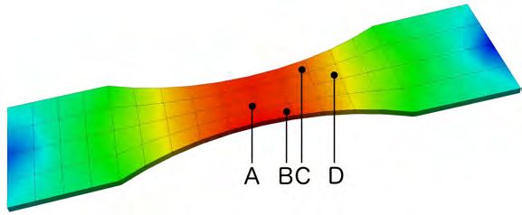
DOMAIN DECOMPOSITION IN COMPUTATIONAL HOMOGENIZATION 3
Recent nonlinear domain decomposition approaches can also be used as, e.g., AS-
PIN [13, 42, 31, 14, 30, 28, 27, 26] or Nonlinear-FETI-DP [35, 33, 40] and the related
Nonlinear FETI-1 or Neumann-Neumann methods [49, 11]. In our implementation
of the FE2 method, the FE2TI package, we focus on Newton-Krylov-FETI-DP and
Nonlinear-FETI-DP approaches. We can, however, currently use also PARDISO [51],
UMFPACK [15], MUMPS [2], or the algebraic multigrid implementation Boomer-
AMG [29, 4] from the hypre [20] package. Fast Fourier transform (FFT) based solvers
would also be possible for structured meshes but are out of the scope of this paper;
see the discussion in section 3.
Domain decomposition methods of the FETI-DP type are fast solvers for linear
and nonlinear problems in solid and structural mechanics and highly scalable to half
a million cores [35] and beyond [36]. BoomerAMG is also highly scalable [3], also for
linear elasticity [4] if improved interpolations are used.
Using parallel solvers for the microscopic boundary value problems (BVPs) results
in several levels of parallelism. On the first level, we have the independent RVEs, each
attached to a Gauß integration point of the macroscopic problem. On the second level,
a parallel approach for the solution of the nonlinear PDEs on the RVEs or SSRVEs
is used. Third, we will also consider parallelization of the macroscopic problem.
2.1. Description of the FE2 approach. Our description of the computa-
tional homogenization FE2 method follows [57], and more details can be found in [23,
57]; also see our earlier works on computational homogenization in the EXASTEEL
project [34, 36, 7]. A similar description can also be found in the dissertation [45].
We first assume that we have a macroscopic boundary value problem or, more
precisely, a problem from the field of solid mechanics with typical length scale L.
The characteristic length scale of the microstructure of the material is defined by l.
Therefore, we assume that the microscopic and heterogeneous structure of the material
can be resolved in the scale l and that L is larger by orders of magnitudes, i.e., L
l.
Additionally, we assume that we have a representative volume element (RVE), which
can effectively describe the microscopic and heterogeneous material properties. The
detailed discussion of the notion of a representative volume element [57] is out of the
scope of this paper.
Based on the underlying assumptions, it is sufficient to discretize the macroscopic
BVP on a domain B with finite elements in the scale of L without considering the
microscopic structure. Then, at each Gauß point of the macroscopic finite elements,
a microscopic BVP, representing the microstructure, is attached. To define an appro-
priate microscopic BVP, a finite element discretization of the RVE in the scale of the
microstructure l is necessary. The appropriate boundary conditions are induced from
the macroscopic deformation gradient at the corresponding Gauß point. A related
method for multiscale problems, more established in the mathematical community, is
the Hierarchical Multiscale Method (HMM) [17, 1]. A recent interesting paper [18]
highlights the close relations to the FE2 method.
Throughout this paper, we will mark macroscopic quantities with bars, as, e.g.,
the deformation gradient F and the first Piola-Kirchhoff stress tensor P . On the
microscale, we use P for the stress and F for the deformation gradient. We do not
have a phenomenological material law on the macroscale, instead, the macroscopic
quantities are assumed to be volumetric averages of quantities on the microscale.
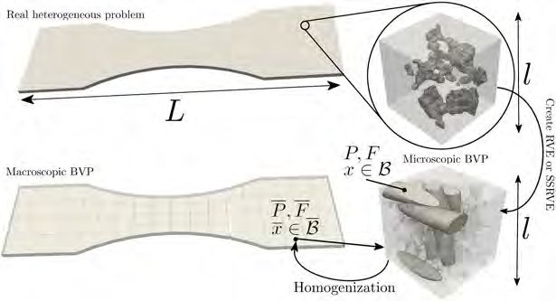
In Figure 1, a schematic illustration of the homogenization approach FE2 is given.
Let us remark that in recent years an approach to reduce the computational effort
of an FE2 simulation was to use RVEs with simplified geometries, e.g., consisting of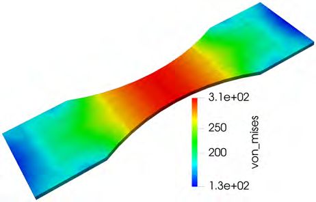
4              A. KLAWONN, S. KÖHLER, M. LANSER, AND O. RHEINBACH

     Fig. 1. Illustration of the FE2 homogenization approach. Top left: Realistic and heterogeneous
macroscopic boundary value problem of length scale L. Top right: Zoom into the microstructure
of the material of length scale l; we have L  l. From the microstructure, an RVE or SSRVE can
be constructed (see bottom right for SSRVE). Bottom Left: Macroscopic and simplified boundary
value problem on the domain B with quantities P and F . The deformation gradient F induces the
boundary conditions of the microscopic BVP on the right. Bottom right: Microscopic boundary
value problem on domain B, which can be an RVE or SSRVE.

ellipsoids; see [52, 53]. These statistically similar RVEs (SSRVEs) can be discretized
with a coarser mesh. In Figure 1, we depict a typical RVE (top right) as well as a
typical SSRVE (bottom right).

    2.1.1. Microscopic boundary value problems. We first introduce the mi-
croscopic boundary value problem defined on a reference configuration B0 and with
corresponding reference variables X. Let us assume that in a deformed state B, the
deformation of our reference configuration can be described by ϕ : B0 → B and the
deformation gradient is defined by F := ∇ϕ. Then, without any further external
forces, the balance of momentum in a weak formulation with a variational function
δx writes
                             Z
(1)                       −      δx · (DivX P (F )) dV = 0.
                                   B0

The tensor P (F ) is the first Piola-Kirchhoff stress tensor and in contrast to the
macroscale, the relation between P and F has to be described by a phenomenological
material law, which describes the considered material sufficiently.
     In our numerical experiments, we consider dual-phase steels and use a J2-elasto-
plasticity model as a material law on the microscale. Work on crystal plasticity is in
progress. The parameter choices and different yield stresses for the martensitic and
ferritic phases can be found in [12, Fig. 10]. The nonlinear equation (1) is then solved
by Newton’s method. More precisely, we typically apply a Newton-Krylov-FETI-DP
or Nonlinear-FETI-DP approach to (1); see section 3 for details.
     As mentioned before, the boundary conditions on the microscale are induced
from the macroscopic deformation gradient F at the corresponding Gauß integration
point. In the case of Dirichlet conditions, we simply enforce x := F X for each
boundary node X ∈ ∂B0 on the microscale. Here, X are the variables in the reference
configuration B0 and x the variables in the deformed configuration B. As many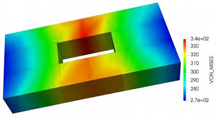
DOMAIN DECOMPOSITION IN COMPUTATIONAL HOMOGENIZATION                       5

homogenization approaches do, the FE2 method assumes that the material can be
characterized sufficiently by a repetitive periodic RVE and therefore the use of periodic
boundary conditions is more reasonable. We first split the boundary ∂B into two parts

                                         ∂B = ∂B + ∪ ∂B − .

For each node X + ∈ ∂B + exists an associated X − ∈ ∂B − and both have opposing
outer normal vectors. With fluctuation fields w̃+ = x − F X + and w̃− = x − F X − we
enforce the periodic boundary condition

                    w̃+ = w̃− ∀ pairs X + ∈ ∂B + and X − ∈ ∂B − .

To obtain regular systems, we additionally enforce w̃+ = w̃− = 0 in the eight corners
of each RVE.
     2.1.2. Homogenization and macroscopic boundary value problem. Sim-
ilarly to the microscopic boundary value problems, we can formulate the macroscopic
problem in a given reference configuration B 0 and reference variables X. Again, the
balance of momentum in the weak formulation with a test function δx writes

                          Z
(2)                                δx · (DivX P (F ) − f ) dV = 0,
                              B0

where f is a volume force. We here disregard surface forces for simplicity.
      On the macroscale, we do not have a material law to deliver an explicit relation
between the deformation gradient F and the stress tensor P . Instead, the first Piola-
Kirchhoff stress tensor P at a macroscopic Gauß point is obtained by homogenization,
i.e., as a volumetric average over the Piola-Kirchhoff stresses P of the corresponding
RVE. Therefore, we have
                                         Z
                                       1
(3)                              P :=        P (F ) dV.
                                       V B0

With (3) and the fact that we consider nonlinear material laws on the microscale,
also (2) is nonlinear in the desired solution F . Thus, also on the macroscale, a
Newton approach is used to solve (2). Standard techniques for the globalization of
Newton’s method can be applied. In our computations, load stepping (pseudo time
stepping) is utilized as a homotopy method; see below.
     Let us briefly derive the Newton iteration formulated in the macroscopic displace-
ment u, such that F = ∇ϕ = I + ∇u, where I is the identity and ϕ the macroscopic
deformation. We assume that we have an initial value u(0) . Given finite element shape
functions NT and their derivatives BT , we can derive a nonlinear residual in the k-th
iteration of Newton’s method on a certain finite element from (2):
                                Z
                                        T   h               T
                     rT u(k) :=       BT P I + u(k) − NT f dV.
                                         T
        h
Here, P marks the discretized stress tensor on element T available in all Gauß points
of the element. For the macroscopic tangent, we then have

                                           Z
                               (k)                T   h
(4)                   dk T u             =       BT A         I + u(k) BT dV,
                                             T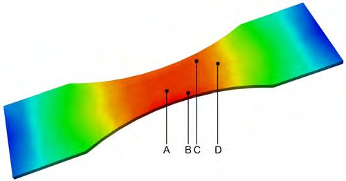
6             A. KLAWONN, S. KÖHLER, M. LANSER, AND O. RHEINBACH

        h
where A is the discretized macroscopic tangent modulus, which again writes
                                                                  Z
                                 ∂P    ∂                      1
(5)                         A :=    =                                      P (F )dV
                                 ∂F   ∂F                      V     B0

and is thus defined in each Gauß point. Using standard finite element routines
                                                                               to
assemble the tangent DK u(k) from dk T u(k) and R u(k) from rT u(k) , we


obtain the Newton iteration
                                             −1
(6)                   u(k+1) = u(k) − DK u(k)     R u(k) .

We now provide a brief description how to compute A. Let us therefore remark
that F is constant on a single RVE. We assume a decomposition of the microscopic
deformation gradient F =: F + Fe on a single RVE into F and a fluctuating part Fe.
Using the chain rule and (3), this immediately leads to
                                       Z                                 Z
                ∂P    ∂             1                                  1          ∂P (F ) ∂F + Fe
(7)      A :=      =                           P (F ) dV           =                     :        dV
                ∂F   ∂F             V    B0                            V     B0    ∂F       ∂F
                            Z                        Z
                        1                        1                 ∂ Fe
(8)                 =               A dV +                A:            dV ;
                        V   B0                   V   B0            ∂F

see also [57, equation (89)]. The first term in the sum (8) is a volumetric average over
the tangent modulus A of the microscopic problem.
     We only have to compute P and A after Newton’s method has converged on
the microscale. Therefore, we can assume an equilibrium state of the weak formu-
lation in (1). Exploiting this fact and using the finite element basis of the RVE, a
                                                      h
reformulation of the discretized tangent modulus A was provided in [57, Section 3.2]:
                                     Z         !
                      h      1 X                    1
(9)                  A :=                A dV − LT (DK)−1 L.
                                          h
                            V         T             V
                                        T ∈τ

Here, τ is the finite element discretization of B0 into finite elements and Ah the discrete
microscopic tangent modulus defined in the Gauß points of the finite elements. Then,
                                             Z         !
                                    1 X           h
                                                A dV
                                    V         T   T ∈τ

                                                     1
                                                          R
is simply the discrete representation of             V        B0
                                                                   A dV in (8). The second term in (9)

                                               1 T
(10)                                             L (DK)−1 L
                                               V

is the discrete form of V1 B0 A : ∂∂FF
                           R
                                         dV exploiting the balance of momentum on
                                     e

the microscale; see [57] for the derivation. Here, the tangential matrix DK of the
microscopic BVP is obtained from assembly of finite element matrices
                                       Z
                                kT :=     BTT Ah BT dV,
                                                     T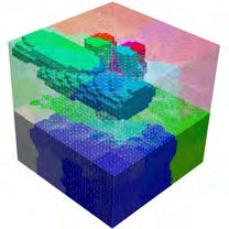
DOMAIN DECOMPOSITION IN COMPUTATIONAL HOMOGENIZATION                           7

where T ∈ τ are finite elements and BT are the derivatives of the shape functions.
The matrix L has to be assembled also from the element contributions
                                      Z
                                lT :=    Ah BT dV.
                                          T

Here, L has the dimension n × s, where n is the number of degrees of freedom in the
RVE and s = 4 in two dimensions and, respectively, s = 9 in three spatial dimensions.
     Let us remark that DK is simply the tangent in the final Newton step on the
RVE and thus the application (DK)−1 L can be interpreted as solving a linear system
with s right hand sides. If a direct solver is used, a mode for multiple right hand sides
can be used or s additional forward backward substitutions have to be performed.
However, if using an iterative solver such as a Nonlinear- or Newton-Krylov-FETI-
DP method, the iterative solver has to be called s times; of course, information reuse
and recycling techniques can be applied to reduce computational cost for the later
iteration phases; see section 4 for details.
     We finally provide an algorithmic description of a single load step of the FE2TI
method in Figure 2, where a Nonlinear- or Newton-Krylov-FETI-DP type method is
used to solve the microscopic RVEs. Let us remark that usually the desired macro-
scopic deformation cannot be applied in a single step but has to be applied in several
consecutive load steps. This often is denoted as pseudo time stepping. The step shown
in Figure 2 has to be repeated for each load step with increasing load. It is possible
to use the solution un from the n-th load step plus additional Dirichlet boundary
                                  (0)
conditions as an initial value un+1 for the Newton iteration in the (n + 1)-th load
step. Alternatively, an extrapolation approach using several former solutions can be
beneficial; see also section 4. Let us remark that we do not consider volume forces f
in this paper but prescribe a fixed deformation as Dirichlet boundary conditions on
parts of the boundary ∂B 0,D ⊂ ∂B 0 in incremental load steps.
   2.2. Implementation remarks. We have implemented the FE2TI package in
PETSc 3.5.2 [5] using C/C++ and MPI.
     2.2.1. Solving the macro problem. In most of our numerical examples, the
macroscopic problem is solved by a sparse direct solver, i.e., UMFPACK or MUMPS,
where this is still feasible. In this case, we solve the macroscopic problem redundantly
on all MPI ranks. For large FE2 simulations, the macroscopic problem can also be
solved in parallel. We can use a Krylov method combined with, e.g., an algebraic
multigrid (BoomerAMG) approach from the hypre library [29] as a preconditioner.
Here, the Krylov subspace method and the AMG preconditioner will run on small MPI
communicators obtained by an MPI Comm split, the macro problem is thus solved
redundantly on the subcommunicators. A parallel domain decomposition method
could also be applied on the macroscale but this approach has not been utilized in
this paper. We often reuse the communicators created for the microscopic solvers
(see below for details), but for small RVEs an additional split into communicators of
efficient size is also possible. The complete macroscopic solution is finally collected on
all MPI ranks of the subcommunicator and thus all MPI ranks. Let us also remark
that the assembly process of the macroscopic problem is also parallelized and, as
should be expected, scales perfectly.
    2.2.2. Solving the micro problems. For each Gauß point of the macroscopic
problem and thus for each microscopic problem, we introduce a separate MPI commu-
nicator. In our implementation, we use MPI Comm split to create subcommunicators
8 A. KLAWONN, S. KÖHLER, M. LANSER, AND O. RHEINBACH
Choose initial macroscopic deformation F which fulfils the boundary conditions
Repeat until convergence (Newton iteration):
1. Apply boundary conditions to RVE based on macroscopic deformation gradient; e.g.
enforce x = F X on the boundary of the microscopic problem ∂B in the case of Dirichlet
constraints.
2. Solve microscopic nonlinear boundary value problem using Nonlinear-FETI-DP, Newton-
Krylov-FETI-DP, or related methods.
3. Compute and return macroscopic stresses as volumetric average over microscopic stresses
P h:
1 X
Z
h h
P = P dV.
V T ∈τ T
4. Compute and return macroscopic tangent moduli as average over microscopic tangent
moduli Ah :
h 1 XZ h 1 T −1
A = A dV − L (DK) L
V T ∈τ T
V
5. Assemble tangent matrix and right hand side of the linearized macroscopic boundary
h h
value problem using P and A .
6. Solve linearized macroscopic boundary value problem.
7. Update macroscopic deformation gradient F .
Fig. 2. Algorithmic description of the FE2TI approach. Overlined letters denote macroscopic
quantities. Blue parts are computations on the microscale and thus the MPI subcommunicators
obtained by MPI Comm split. Red parts are macroscopic computations performed on all MPI ranks.
Algorithmic description taken from [36].
of equal size. Inter-communicator communication is not necessary during the micro-
scopic solves and the averaging of the different microscopic quantities; see points 1 to 4
in Figure 2. To solve the microscopic BVPs, we use a Nonlinear- or Newton-Krylov-
FETI-DP method; see section 3 for details.
In order to compute LT (DK)−1 L (see (9)), we solve s linear systems with DK
as left hand side, i.e., we have nine right hand sides in 3D or four right hand sides in
2D. If an iterative solver is used, this can be an expensive step and, in extreme cases,
in our numerical experiments, the computation of the consistent tangent moduli can
take up more than 50% of the total time to solution. Approximating LT (DK)−1 L or
even discarding the matrix LT (DK)−1 L completely can be feasible alternatives even
though superlinear convergence may be lost for the macroscopic problem.
A discussion of different strategies is provided in section 4. Finally, we use collec-
h h
tive communication to provide A and P on all MPI-ranks in order to assemble the
linearized macroscopic problem (6). This is efficiently performed by first collecting
and summing up all averaged values on the first rank of each microscopic subcom-
municator and a consecutive collection step using only those first ranks. Thereby,
we avoid global communication involving all MPI ranks but only communicate on
independent subsets of MPI ranks at the same time.
3. Parallel domain decomposition solvers. We use iterative multilevel meth-
ods to solve our nonlinear solid mechanics problems on the RVEs, i.e., mostly parallel
domain decomposition methods of the linear or nonlinear FETI-DP type or alge-
braic multigrid. Our implementations of nonlinear FETI-DP domain decomposition
methods, developed within the SPPEXA EXASTEEL project, have scaled to the
full 786 432 cores [36] of the Mira BG/Q Supercomputer (Argonne National Labo-
ratory, USA) for a heterogeneous nonlinear hyperelasticity problem with 60 billion
unknowns; also see [35], for details on the method and implementation. In [35],
also results for nonlinear domain decomposition on the SuperMUC supercomputerDOMAIN DECOMPOSITION IN COMPUTATIONAL HOMOGENIZATION 9
(LRZ, Munich, Germany), the Vulcan supercomputer (Lawrence Livermore National
Laboratory, USA), and the JUQUEEN supercomputer (JSC, Jülich, Germany) are
included. For robustness, especially for heterogeneous problems, we usually apply
sparse direct solvers, i.e., PARDISO [51], UMFPACK [15], or MUMPS [2] as local
subdomain solvers. Here, to speed up the Krylov iteration phase, accelerating the
forward-backward substitution in the sparse direct solver is of interest [62]. In our
implementation it is also possible to use efficient preconditioners such as multigrid for
the local problems in nonlinear domain decomposition; see [37, 38]. Shared-memory
parallelization on the node is an option in our software if a shared-memory parallel
subdomain solver (such as PARDISO or BoomerAMG) are used; see [39]. There,
parallelization of the finite element assembly, combining PETSc and OpenMP, and
the solution of the subdomain problems, using PARDISO, was performed. Good scal-
ability using up to four OpenMP threads for each MPI rank on an Intel Ivy Bridge
architecture was observed and incremental improvements were obtained using up to
ten threads.
For voxel meshes, see, e.g., Figure 3 and Figure 4, geometric multigrid methods
or Fast Fourier (FFT) transform based solvers would be efficient alternatives, since
they can profit from the tensor structure of such meshes. In [19], the authors com-
pare an FFT-based solution method with standard Q1 finite elements for a crystal
plasticity problem defined on an RVE. As the FFT-based method exploits the ten-
sor structure of the problem, the authors use structured meshes (voxel meshes) for,
both, the FFT-based approach as well as for the Q1 finite element meshes. For the
FEM problems, a commercial code was applied. The authors concluded that with re-
spect to computational cost the FFT-based approach can be computationally cheaper
by one to two orders of magnitude. Indeed, FFT-based computational homogeniza-
tion approaches have successfully been used by different authors in recent years; see,
e.g., [59, 32, 55, 43, 54, 16] and references therein. The FFT approaches are valued
for the high efficiency when applied to voxel-based RVEs with millions of degrees of
freedom, and because voxel meshes from EBSD measurements, as in Figure 3, can
directly be used without further processing. However, in FFT homogenization, e.g.,
based on [48], the number of iterations will depend on the contrast; see, e.g., [32].
Note that the approach presented in this paper differs from other approaches,
including those using FFT solvers on the microscale. In order to obtain better ap-
proximations on the microscale, especially for plasticity, we use second order (P2) fi-
nite elements instead of simple linear tets (P1) or trilinear hexahedral elements (Q1).
We then use an approach (SSRVEs) to construct RVEs using simple geometries, e.g.,
ellipsoids. However, the advantages of SSRVEs can only be exploited fully when us-
ing unstructured meshes, and we therefore use unstructured tetrahedral meshes, well
adapted to the geometry. Our parallel domain decomposition methods can cope with
these unstructured meshes, and the number of Krylov iterations will be only slightly
higher. We also use direct sparse solvers on the subdomains for high robustness of the
numerical methods and usually obtain quadratic convergence of the overall Newton
scheme; cf. Figure 18. We will see in our numerical results that, for our SSRVEs, un-
structured meshes are clearly favorable; see subsection 4.2. We will also see that the
unstructured meshes can also be allowed to be significantly, i.e., more than an order
of magnitude, smaller than the structured meshes. Using adaptive mesh refinement
could further expand the advantage but this is out of the scope of this paper.
Recent versions of PETSc include an efficient implementation of iterative sub-
structuring methods [63]. However, we apply our own parallel implementation [35, 41]
which is earlier and also includes our most recent versions of nonlinear domain de-10 A. KLAWONN, S. KÖHLER, M. LANSER, AND O. RHEINBACH
composition methods [40].
Let us briefly describe the linear and nonlinear FETI-DP domain decomposition
methods, which we will utilize to solve the RVE problems on the microscale. In
our computational homogenization approach, the micro problems are usually more
challenging than the macro problem as a result of the heterogeneities, which have to
be homogenized.
3.1. Parallel linear and nonlinear domain decomposition of FETI-DP
type. Given a nonoverlapping domain decomposition Ω1 , . . . , ΩN of the computa-
tional domain Ω ⊂ R3 , we introduce the (generally) nonlinear operators K1 , . . . , KN ,
defined on the subdomains, and the corresponding right hand sides f1 , . . . , fN . In
nonlinear domain decomposition, we usually obtain the operators K1 , . . . , KN from
the minimization of a nonlinear (e.g., hyperelastic) energy on the subdomains; see [33,
equation (2.4)]. In Newton-Krylov-DD methods, the operators K1 , . . . , KN are linear
as the domain decomposition is performed after Newton linearization.
In our FE2 simulations, the domain Ω will be an RVE B0 and K1 , . . . , KN as well
as f1 , . . . , fN are determined by (1). We define the block vectors u = (u1 , . . ., uN ),
K(u)T = [K1 (u1 )T . . . KN (uN )T ]T , f T = [f1T , . . . fN
T T
] .
T
Using the partial finite element assembly operator RΠ in primal variables, we obtain
the partially assembled nonlinear operator K,
e
e u) = RT K(RΠ ũ)
K(e Π
and the corresponding right hand side f˜ = RΠ T
f. As in linear FETI-DP methods,
the global coupling by partial finite element assembly is introduced to make the local
problems invertible and to obtain numerical scalability. As a result, the Jacobian
DK(ũ)
e can be assumed to be invertible, while it still maintains a favorable, partially
decoupled, structure, i.e.,
(1) e (1) (ũ)
DKBB (ũ) DK BΠ
.. ..
DK(ũ) =
e
. .
.
(N ) (N )
DKBB (ũ) DKBΠ (ũ)
e
DKe (1) (ũ) . . . DK
e (N ) (ũ) DKe ΠΠ (ũ)
ΠB ΠB
We now define nonlinear FETI-DP methods as iterative methods for the solution
of the nonlinear system (see [33, 40])
+ B T λ − f˜
K(ũ)
e 0
(11) A(ũ, λ) := = .
B ũ 0
Since the nonlinear problem K(ũ)
e = f˜ − B T λ can very efficiently be parallelized,
such methods can be highly scalable and nonlinear problems with billions of degrees
of freedom [35] can be solved in a few minutes. As in standard, linear FETI-DP
methods [61, 22, 21, 41] the linear constraint B ũ = 0 enforces the continuity across the
subdomain boundaries, using Lagrange multipliers λ. However, as opposed to linear
FETI-DP methods, the continuity is only achieved at convergence of the Newton
iteration; see [33] for details.
The (generally) nonlinear system (11) can be solved using different strategies;
see [40]. These methods are all equivalent to the classical FETI-DP method if K is a
linear operator.DOMAIN DECOMPOSITION IN COMPUTATIONAL HOMOGENIZATION 11
#subdomains unstructured meshes structured meshes
#elements #degrees of freedom #elements #degrees of freedom
30 23 537 103 266 20 480 95 523
64 47 296 199 125 69 120 311 475
110 222 489 921 648 214 375 945 108
Table 1
Meshes for the SSRVEs. We use P2 finite elements.
For our problems on the RVEs, we can apply Newton’s method directly to (11).
This was denoted Nonlinear-FETI-DP-1 in [33]. We will either use a classical Newton-
Krylov FETI-DP approach, i.e., the microscopic BVP is first linearized and the FETI-
DP method is applied to the linearized system, or Nonlinear-FETI-DP-1 is used, i.e.,
T
Newton linearization is applied to (11), and the Newton correction δ ũ(k) ; δλ(k) can
be computed from
δ ũ(k) e (k) ) + B T λ(k) − f˜
e (k) ) B T
DK(ũ K(ũ
(12) = .
B 0 δλ(k) B ũ(k)
A reduction to the Lagrange multipliers leads to a linear system of the form
(13) F δλ(k) = d,
which is solved iteratively by a Krylov method, e.g., GMRES, throughout this paper,
preconditioned by the standard FETI-DP Dirichlet preconditioner [61].
4. Numerical results. If not marked otherwise, we use a Newton-Krylov-FETI-
DP approach for the solution of the microscopic RVE problems, i.e., we have used
the most conservative choice among our FETI-DP methods. We also present re-
sults using Nonlinear-FETI-DP-1 on the Theta supercomputer later on. This is the
most conservative choice among the recent Nonlinear-FETI-DP and Nonlinear-BDDC
methods [35, 33, 40]. In our numerical experiments, if not denoted otherwise, the
macroscopic problem is discretized using piecewise linear triangular elements (P1) in
2D and piecewise trilinear or quadratic brick elements (Q1 or Q2) in 3D. In all our
experiments we stop the macroscopic Newton iteration if the norm of the update is
smaller than 1e − 6. We use a tolerance of 1e − 8 for the microscopic Newton iteration
and use a relative stopping tolerance of 1e − 9 for all Krylov subspace methods.
We use computing time on the JUQUEEN supercomputer (Jülich Supercomput-
ing Centre), a large BG/Q (PowerBQC 16C 1.6 Ghz) installation with a total of
458 752 cores and 1 GB of memory for each core. JUQUEEN was Europe’s fastest
supercomputer in 2015 and is still ranked 22nd in the TOP500 list of November 2017.
4.1. Simulation using a voxel-based RVE from EBSD measurements. In
this section, we consider FE2 simulations using a structured mesh based on voxel data
obtained from EBSD (Electron Backscatter Diffraction) measurements as an RVE.
We use P2 finite elements on the microscale, where each voxel is decomposed into six
ten-noded tetrahedra. The RVEs consisting of 663 552 finite elements and 2 738 019
degrees of freedom. Each RVE is decomposed into 512 subdomains. We consider a
plate with a hole discretized with 64 finite elements and thus using 512 RVEs. The
sum of the number of degrees of freedom on the microscale is thus approximately
1.4 billion. We simulate four different deformations. We twist the plate and apply
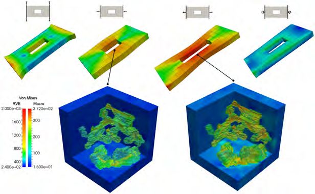
different pulling and pressing forces; see Figure 3 (top).12 A. KLAWONN, S. KÖHLER, M. LANSER, AND O. RHEINBACH
Fig. 3. Four different types of macroscopic deformations. Simulations performed with RVEs
with 663 552 finite elements and 2 738 019 degrees of freedom. The geometry of the RVEs corresponds
to a small cubic part of a larger structure obtained from EBSD measurements of a dual-phase steel.
The computations have been performed with 262 144 MPI ranks on 131 072 cores of JUQUEEN.
Based on data from [12].
Each of the simulations has been performed using 262 144 MPI ranks using 131 072
cores of the JUQUEEN supercomputer. The numerical scheme remained stable and
reliable results have been obtained; see Figure 3. The I/O-time to write all data for
all RVEs to the file system always stayed below 2% of the total runtime.
These results show the scalability of the FE2TI package and demonstrate its
ability to run efficiently on large supercomputers, consistent with the earlier results
from [34, 36, 7]. Therefore, in the following sections, we fokus on further optimizing
and tailoring the RVE solver. We also investigate if we can reduce the size of the
RVEs.
4.2. Considering different discretizations of the microscale. In this sec-
tion, we study the influence of the structure and resolution of the discretization of
a chosen RVE or SSRVE on the homogenized solution on the macroscale. The con-
struction of the SSRVEs using a fixed number of ellipsoidal inclusions based on EBSD
measurements is discussed in [53]; also see [12]. Nonetheless, the resolution of the
discretization of the SSRVEs is comparably coarse in [53]. Here, we present a com-
parison of macroscopic and microscopic results using meshes of different refinement
levels; see Figure 4 and Figure 5 for different SSRVE meshes. We consider structured
grids (Figure 4), which cannot resolve the ellipsoidal inclusions very well, as well as
unstructured grids (Figure 5). These investigations also provide us with a grid conver-
gence study. As a macroscopic problem, we extend a symmetric plate discretized with
72 finite elements in x-direction; see Figure 6 (left) for the undeformed geometry. We
first apply 11 load steps with a deformation of 0.025 percent of the current deformed
state in each load step; see Figure 6 (right) for a visualization of the load.
For our meshes, see Table 1. Our largest unstructured mesh, discretizing the
SSRVE using two ellipsoids [53], consists of 222 489 finite elements (see Figure 5 right)
and is chosen as our reference. When we to refer to the error (see Figure 8), we mean
the difference to the solution on the reference mesh.DOMAIN DECOMPOSITION IN COMPUTATIONAL HOMOGENIZATION 13
In Figure 7, we present the von Mises stresses in the macroscopic problem after
11 load steps using the reference discretization. To compare the effects of using
different SSRVE meshes on the macroscopic results, in Figure 8, we depict the relative
difference in the von Mises stresses between the reference solution from Figure 7 and
solutions obtained using coarser unstructured and structured grids.
For the unstructured grids – see Figure 8 (rows four to five) – we see only small
differences for both grids and also observe convergence to the reference solution from
the coarser grid (row four) to the finer one (row five). On the other hand, we obtain
significant differences using structured grids, even though the finest structured SSRVE
is of the same size as the unstructured reference SSRVE; see Figure 8 (rows one
to three). Therefore, we can conclude that the choice of the discretization of the
SSRVE has a significant impact. Our unstructured grids result in a significant better
approximation of the reference solution than all structured grids, even if the number
of finite elements is an order of magnitude smaller.
All in all, in our experiments, the von Mises stresses have been slightly higher
when structured grids are used. First, this is a result of high stress peaks caused by
the unsmooth resolution of the surfaces of the ellipsoids. Second, the minimal stresses
in the SSRVEs appear to be slightly higher in the case of structured meshes. The
first effect can be observed in the stress distributions in Figure 9, where we depict the
unstructured SSRVE alongside the structured ones. In Figure 9, four different Gauß
points A,B,C, and D are considered as well as two different grid resolutions.
We additionally provide data on the stress peaks and the average stresses in
Gauß points A and C in Figure 10 (left and middle). The second effect is depicted
in Figure 10 (right) for the same two Gauß points A and C.
Fig. 4. Structured discretization with similar numbers of finite elements as the unstructured
in Figure 5 and domain decomposition of an SSRVE with two ellipsoidal inclusions. The colors show
the decomposition of the lower half of the cube and the ellipsoids. Left: 20 480 finite elements and
30 subdomains. Middle: 69 120 finite elements and 64 subdomains. Right: 214 375 finite elements
and 110 subdomains.
4.3. Improvements of the numerical scheme. In this section, we study tech-
niques to improve the efficiency of our simulation. We also discuss the use of an
approximate tangent in the solution of the macroscopic problem.
Our macroscopic test problem in this section consists of only 16 macroscopic
finite elements, resulting in 128 microscopic RVE problems. Here, we always use
the unstructured SSRVE with 47 296 finite elements decomposed into 64 FETI-DP
subdomains; see Table 1. In this section, a 1% deformation in x-direction using 21
load steps was applied on the macroscale; see also Figure 11 for the macroscopic
solution. We keep the stopping criterion of the macroscopic and microscopic Newton
iterations fixed at 1e − 6 and, respectively, 1e − 8. We keep the relative stopping14 A. KLAWONN, S. KÖHLER, M. LANSER, AND O. RHEINBACH
Fig. 5. Unstructured discretization and domain decomposition of an SSRVE with two ellipsoidal
inclusions. The colors show the decomposition of the lower half of the cube and the ellipsoids. Left:
23 537 finite elements and 30 subdomains. Middle: 47 296 finite elements and 64 subdomains.
Right: 222 489 finite elements and 110 subdomains.
Fig. 6. Macroscopic Problem. Left: undeformed Geometry; Right: scaled deformation (factor
50) after 10 steps.
criterion of the FETI-DP solver at 1e − 9 since the high accuracy is necessary for fast
Newton convergence on the microscale.
We consider three improvements of our numerical scheme.
1. Lambda-recycling in FETI-DP: We reuse the solutions λ of earlier Newton
steps as initial values for the FETI-DP solvers; see (13).
2. Approximate tangent modulus: We vary the stopping tolerance for the linear
FETI-DP solves necessary for the computation of the consistent macroscopic tangent
moduli; see (10). Stopping early leads to an approximate tangent on the macroscale.
3. Extrapolation on the macroscale: We use an extrapolation approach to obtain
a proper initial value for the Newton iteration on the macroscale.
Lambda-recycling in FE2TI. In general, the idea of lambda-recycling in Newton-
Krylov-FETI-DP is to use the solution λ(k) of the linear system from the k-th Newton
iteration as an initial value for FETI-DP in the (k + 1)-th Newton iteration, e.g., to
compute λ(k+1) . In FE2TI, we apply Newton-Krylov-FETI-DP on each RVE in each
macroscopic step and use lambda-recycling on each RVE individually. Additionally,
we use the solution from the last Newton-Krylov-FETI-DP iteration of the previous
macroscopic step as an initial value for the first Newton-Krylov-FETI-DP iteration
of the current macroscopic step. Let us remark that nonlinear FETI-DP methods do
not need any lambda-recycling strategies since the reuse of information automatically
arises from the nonlinear scheme.
It is interesting to note that when solving for the nine right hand sides in (13),
these right hand sides are rather different and the lambda-recycling approach between
those nine solves does not seem to be beneficial. It turns out that it is more efficient to
use lambda-recyling from the nine individual solutions from the previous macroscopic
iteration. This strategy is thus included in the FE2TI package.
Approximate tangent modulus in FE2TI. The nine additional linear FETI-DP
solves to obtain a consistent tangent modulus and thus a consistent tangent on theDOMAIN DECOMPOSITION IN COMPUTATIONAL HOMOGENIZATION 15
Fig. 7. Von Mises stresses after 10 load steps using the largest of the three SSRVE.
Fig. 8. Pointwise relative error in von Mises stresses on the macroscale using different SS-
RVEs after 7 (left column) and 11 load steps (right column). The reference solution is obtained
using a large SSRVE with an unstructured mesh (see bottom right in Figure 5). For the results in
the first three rows, we use SSRVEs with structured meshes and for the last two rows SSRVEs with
unstructured meshes - First row: SSRVE with structured mesh decomposed into 30 subdomains and
20 480 finite elements. Second row: SSRVE with structured mesh decomposed into 64 subdomains
and 69 120 finite elements. Third row: SSRVE with structured mesh decomposed into 110 subdo-
mains and 214 375 finite elements. Fourth row: SSRVE with unstructured mesh decomposed into
30 subdomains and 23 537 finite elements. Fifth row: SSRVE with unstructured mesh decomposed
into 64 subdomains and 47 296 finite elements.16 A. KLAWONN, S. KÖHLER, M. LANSER, AND O. RHEINBACH
Fig. 9. From left to right: von Mises stresses in four Gauß points A,B,C, and D after 10
load steps - the locations of the points A to D is depicted above. The deformation of the SSRVEs
is scaled by a factor of 20. Rows one and two: coarse structured and unstructured discretizations
with 20 480 and, respectively, 23 537 finite elements, both decomposed into 30 irregular subdomains.
Rows three and four: fine structured and unstructured discretizations with 214 375 and, respec-
tively, 222 489 finite elements, both decomposed into 110 irregular subdomains.
macroscale (see (13)) can exhibit a significant portion of the runtime, especially when
using iterative solvers. Nevertheless, it is necessary in order to obtain quadratic con-
vergence of Newton’s method on the macroscale. We suggest to reduce the accuracy
of the nine linear solves and thus use an approximate tangent on the macroscale. We
therefore tested different stopping tolerances for FETI-DP for the computation of the
consistent tangent modulus.
Extrapolation of macroscopic solutions in FE2TI. This approach is rather simple.
If an extrapolation of the macroscopic iterates is activated in the FE2TI package, theDOMAIN DECOMPOSITION IN COMPUTATIONAL HOMOGENIZATION 17
Fig. 10. Maximal stress (left), average stress (middle), and minimal stress (right) after 10
load steps in structured and unstructured SSRVEs attached to Gauß points A and C - see Figure 9
for location of Gauß points; see Table 1 for the number of finite elements.
Fig. 11. Macroscopic solution of a small model problem after 17 load steps.
(0)
initial value for the (k + 2)-th macroscopic load step umacro,k+2 is chosen as a linear
extrapolation from the solutions of the k-th and (k + 1)-th load steps u∗macro,k and,
respectively, u∗macro,k+1 , i.e.,
(0)
umacro,k+2 = 2u∗macro,k+1 − u∗macro,k .
4.4. Effects of the improvements. Without any of the improvements intro-
duced in the previous section, the FE2 simulation takes 10 445.5s to perform 21 macro-
scopic load steps using a total of 82 macroscopic Newton steps. Using lambda-
recycling alone, the runtime can be reduced to 7 693.0s, which is 1.36 times faster.
Choosing different accuracies for the computation of the consistent tangent mod-
ulus (1e − 9, 1e − 6, 1e − 3, 1e − 1), quadratic convergence of the macroscopic Newton
iterations was lost only for 1e − 1, where the total number of Newton iterations in
21 load steps increases slightly from 82 to 88; see also Table 2.
The runtime is reduced from 7 693.0s to 5 573.5s for the tolerance 1e − 3, which
is our best choice and corresponds to a factor of 1.38 of reduction in runtime.
In Figure 12, we provide a comparison of three variants, namely without lambda-
recycling and with lambda-recycling and different tolerances 1e − 9 and 1e − 3 for the
consistent tangent.
Finally, adding the macroscopic extrapolation of solutions, the number of macro-
scopic Newton iterations is further reduced to 66, and thus also the runtime is reduced
to 4 721.0s; see Table 2. Combining all three improvements, we can accelerate the
computations by a factor of 2.2.
4.5. Large run using the improvements. Combining our different strategies,
i.e., λ-recycling, approximation of the consistent tangent moduli, and extrapolation
of macroscopic solutions, we are able to simulate 81 load steps with a 2.1% total18 A. KLAWONN, S. KÖHLER, M. LANSER, AND O. RHEINBACH
Fig. 12. Runtime of the macroscopic Newton iterations. Comparison between FE2TI without
optimization, FE2TI with lambda-recycling, and FE2TI with lambda-recycling plus using an approx-
imate tangent modulus with tolerance 1e − 3. Additionally, the macroscopic load steps are marked
in red on the x-axis.
load lambda stopping tol. Newton It. Total
steps recycling consistent tangent extrapolation Macroscale Runtime
21 no 1e-9 no 82 10 445.5s
21 yes 1e-9 no 82 7 693.0s
21 yes 1e-6 no 82 6 484.2s
21 yes 1e-3 no 82 5 573.5s
21 yes 1e-1 no 88 5 688.5s
21 yes 1e-3 yes 66 4 721.0s
Table 2
Improvements using lambda-recycling, inexact macroscopic Newton’s method, and extrapolation
of the macroscopic problem.
deformation in 4 hours and 39 minutes using 18 432 JUQUEEN cores. Here, we use
the unstructured SSRVE with 47 296 finite elements, since the approximation of the
reference solution showed to be accurate enough. We depict the final state of the
solution in Figure 13.
4.6. Improving scalability by exploiting parallelism on the macroscale.
As mentioned above, the capability to solve the macroscopic problem in parallel with
an iterative Krylov subspace method (e.g., CG or GMRES) and, e.g., the Boomer-
AMG preconditioner [29] was included. When using BoomerAMG, we always use
HMIS coarsening, long range ext+i interpolation, and a nodal coarsening approach;
see [4] for a discussion of efficient parameters for elasticity.
The macroscopic problem is assembled and solved in parallel on a subset of ranks
of the MPI communicators which are assigned to the RVEs. In our tests, these com-
municators have a reasonable size, e.g., 64 MPI ranks if the RVE is decomposed into
64 subdomains. In the following tests, we always use between 2 and 64 MPI ranks and
thus AMG is only applied on a small number of ranks. The result of the macroscopic
problem is distributed to the complete communicator and then available on all MPI
ranks. We perform two different weak scaling tests using the unstructured SSRVE
with 64 subdomains and the best parameter settings found before, i.e., λ-recycling,
approximation of the consistent tangent moduli, and extrapolation of macroscopic
solutions are used.
We perform 13 load steps for an uniaxial tension test of a macroscopic cube. In
the first weak scaling test, we use four MPI ranks for each JUQUEEN core and use up
to 1.04 million MPI ranks; see Figure 14 (top left and top right) and Figure 15 for the
results. The results in Figure 15 show significant improvements using parallelizationDOMAIN DECOMPOSITION IN COMPUTATIONAL HOMOGENIZATION 19
Fig. 13. Von Mises stresses after 81 load steps and a total deformation of approximately 2.1%
of the macroscopic reference configuration. Four SSRVEs A,B,C, and D (from left to right) are
depicted.
of the macro problem.
In the second test, we use two MPI ranks per core and scale up to the complete
machine; see Figure 14 (bottom left and bottom right). Considering the average time
per macroscopic Newton iteration, we obtain an excellent efficiency of 74% on 1.04
million MPI ranks using AMG for the macroscopic problem and, respectively, for the
setup using two MPI ranks per compute core, 78% parallel efficiency on the whole
machine. In both cases the scalability is increased drastically in comparison to the
approach using a direct solver on the macroscale.
4.7. Production runs on Theta using Nonlinear-FETI-DP-1. In this sec-
tion, we present some results for large production runs using Nonlinear-FETI-DP-1
to solve the microscopic problems.
Theta is a large Intel Xeon Phi (Xeon Phi 7230, 64 Cores, 1.3 Ghz, “Knights
Landing”) x86 installation at Argonne Leadership Computing Facility (ALCF) with
a total of 231 424 cores and ranked 18th in the TOP500 list of November 2017. Theta
is a very capable supercomputer. Unfortunately, Intel has discontinued its Xeon Phi
line and Theta’s successor named Aurora, planned to be the first exascale system of
the USA in 2021, will use a different architecture.
Analogously to the last subsection, we use the extrapolation approach and an
approximate consistent tangent. With Nonlinear-FETIDP-1, λ-recycling is not nec-
essary. Indeed, the most conservative nonlinear FETI-DP method – Nonlinear-FETI-
DP-1 – shows to be as robust and efficient as Newton-Krylov-FETI-DP with λ-
recycling.20 A. KLAWONN, S. KÖHLER, M. LANSER, AND O. RHEINBACH
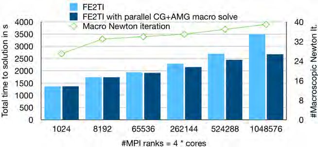
Fig. 14. Top Left: Average Time for each macroscopic Newton iteration scaling to 1.02 mil-
lion MPI ranks on JUQUEEN using CG plus AMG preconditioner or a direct solver, respectively.
Top Right: Corresponding efficiency to runtimes presented in top left figure. Bottom Left:
Average Time for each macroscopic Newton iteration scaling up to the complete JUQUEEN. Bot-
tom Right: Corresponding efficiency to runtimes presented in bottom left figure.
Fig. 15. Weak parallel scalability on JUQUEEN. Total time to solution of FE2TI for 13 load
steps using CG with an AMG preconditioner or, respectively, a direct solver on the macroscale. The
largest problem has 3.3 billion degrees of freedom on the microscale and 7.8 thousand degrees of
freedom on the macroscale.
4.8. First run on Theta. We are able to simulate 171 load steps with a total
deformation of 4.3% in exactly 4 hours walltime using 36 864 cores of Theta (Argonne
National Laboratory, USA). Here, we use the unstructured SSRVE with 47 296 finite
elements (see Table 1) since the approximation of the reference solution showed to be
accurate enough. The problem has 302 million degrees of freedom in the microscale
and 570 degrees of freedom on the macroscale
We depict the final state of the solution in Figure 16 and the development of the
von Mises stresses over time in Figure 17 for six different vertices.
We also show the number of necessary Newton and FETI-DP iterations on the
microscale. In Figure 18 the effect of plastification of certain RVEs can be observedDOMAIN DECOMPOSITION IN COMPUTATIONAL HOMOGENIZATION 21
Fig. 16. Von Mises stresses after 171 load steps and a total deformation of approximately 4.3%
of the macroscopic reference configuration. Four exemplary SSRVEs A,B,C, and D (from left to
right) are depicted.
Fig. 17. Von Mises stress in six vertices of the macroscopic problem over pseudo time.
nicely by observing the number of Nonlinear-FETI-DP-1 and GMRES iterations in
different load steps. Clearly, starting at load step number four, RVEs A and B need
more Newton steps to converge than C and D, which marks the point in time when
these two RVEs start to show a plastic behavior.
This introduces a certain load imbalance and can also be observed in the corre-
sponding runtimes; see Figure 19. This load imbalance shows to be of minor interest
and does not affect the performance of FE2TI severly, since, after approximately 20
load steps, all RVEs in the critical region show a plastic behavior and the load im-
balance vanishes. To illustrate this effect, we also present the Newton iterations and
Nonlinear-FETI-DP-1 runtimes of load steps 70 to 79; see Figure 18 (right) and Fig-22 A. KLAWONN, S. KÖHLER, M. LANSER, AND O. RHEINBACH
Fig. 18. Newton iterations on the microscale for the four RVEs A, B, C, and D (see Figure 13
for position of RVEs); each block of four columns represents a single macroscopic Newton step in a
certain macroscopic load step (marked on the x-axis). Left: Load steps 1 to 10. Right: Load steps
70 to 79.
Fig. 19. Runtime of Nonlinear-FETI-DP-1 on the microscale for the four RVEs A, B, C, and
D (see Figure 13 for position of RVEs); each block of four columns represents a single macroscopic
Newton step in a certain macroscopic load step (marked on the x-axis). Left: Load steps 1 to 10.
Right: Load steps 70 to 79.
ure 19 (right). We also present the number of GMRES iterations per Nonlinear-FETI-
DP-1 solve in Figure 20. The average number of GMRES iterations per linear solve
is approximately 40 for each of the four RVEs, which is a satisfactory result.
4.9. Second run on Theta. We finally present results for a refined macroscopic
mesh with 1 792 SSRVEs computed on Theta using Nonlinear-FETI-DP-1. We sim-
ulate 319 load steps using 114 688 cores of Theta and obtain a deformation of 7.7%
in x-direction. The problem has 693 million degrees of freedom in the microscale
and 1 305 degrees of freedom on the macroscale. Some results for different RVEs and
different load steps are presented in Figure 21.
4.10. Conclusion. We have presented a framework for parallel computational
homogenization using the FE2 approach. The usage of parallel domain decomposition
solvers on the microscale and parallel algebraic multigrid solvers on the macroscale al-
lows large multiscale simulations for micro-heterogeneous media. We have shown FE2
simulations with million-way parallelism and billions of degrees of freedom. Larger
simulations will be possible once exascale supercomputers will become available.
Acknowledgments The authors gratefully acknowledge the Gauss Centre for Supercomputing e.V.
(www.gauss-centre.eu) for providing computing time on the GCS Supercomputer SuperMUC at Leibniz
Supercomputing Centre (LRZ, www.lrz.de) and JUQUEEN [60] at Jülich Supercomputing Centre (JSC,
www.fz-juelich.de/ias/jsc). GCS is the alliance of the three national supercomputing centres HLRS (Uni-
versität Stuttgart), JSC (Forschungszentrum Jülich), and LRZ (Bayerische Akademie der Wissenschaften),
funded by the German Federal Ministry of Education and Research (BMBF) and the German State Min-
istries for Research of Baden-Württemberg (MWK), Bayern (StMWFK) and Nordrhein-Westfalen (MKW).
This research used resources (Theta) of the Argonne Leadership Computing Facility, which is a DOE Office
of Science User Facility supported under Contract DE-AC02-06CH11357. The authors acknowledge the use
of data from [12] provided through a collaboration in the DFG SPPEXA project EXASTEEL.
REFERENCESYou can also read