Analysis of experimental data for the BCI hybrid systems
←
→
Page content transcription
If your browser does not render page correctly, please read the page content below
University of Warsaw
              Faculty of Physics

                Dawid Laszuk
             Student’s book no.: 276909

Analysis of experimental data for the
        BCI hybrid systems
            Second cycle degree thesis
              field of study Physics
         speciality BIOMEDICAL PHYSICS

                         The thesis written under the supervision of
                         dr Rafał Kuś
                         University of Warsaw,
                         Faculty of Physics

              Warsaw, September 2012
Oświadczenie kieruja̧cego praca̧

Oświadczam, że niniejsza praca została przygotowana pod moim kierunkiem i stwierdzam, że spełniła
ona warunki do przedstawienia jej w postępowaniu o nadanie tytułu zawodowego.

Data                                                                           Podpis kieruja̧cego praca̧

 Statement of the Supervisor on Submission of the Thesis

I hereby certify that the thesis submitted has been prepared under my supervision and I declare that it
satisfies the requirements of submission in the proceedings for the award of a degree.

Date                                                                         Signature of the Supervisor

 Oświadczenie autora (autorów) pracy

Świadom odpowiedzialności prawnej oświadczam, że niniejsza praca dyplomowa została napisana przeze
mnie samodzielnie i nie zawiera treści uzyskanych w sposób niezgodny z obowiązującymi przepisami.
Oświadczam również, że przedstawiona praca nie była wcześniej przedmiotem procedur związanych z
uzyskaniem tytułu zawodowego w wyższej uczelni.
Oświadczam ponadto, że niniejsza wersja pracy jest identyczna z załączoną wersją elektroniczną.

Data                                                                                Podpis autora pracy

Statement of the Author(s) on Submission of the Thesis

Aware of legal liability I certify that the thesis submitted has been prepared by myself and does not
include information gathered contrary to the law.
I also declare that the thesis submitted has not been the subject of proceedings resulting in the award of
a university degree.
Furthermore I certify that the submitted version of the thesis is identical with its attached electronic
version.

Date                                                            Signature of the Author(s) of the thesis
Abstract
Interfejsy mózg-komputer (Brain-computer interfaces, BCI) umożliwiają człowiekowi komu-
nikację z komputerem bez pośrednictwa obwodowego układu nerwowego. Chociaż pierwszy in-
terfejs został skonstruowany ponad 20 lat temu, ich szybkość i skuteczność działania jest wciąż
niska. Obecnym trendem badań jest tworzenie hybrydowych systemów poprzez jednoczesne
wykorzystanie kilku paradygmatów BCI lub połączenie ich z innymi interfejsami.
Celem pracy było skonstruowanie hybrydowego interfejsu opartego na tzw. paradygmacie P300
i okulografie oraz opracowanie na jego potrzeby metod analizy danych. Szybkość omówionego
interfejsu wyznaczono na poziomie 86.45 bit/min.      Zaproponowana metoda analizy danych
składa się z filtru przestrzennego Common Spatial Pattern (CSP), liniowej analizy dyskryminacji
Fishera (Fisher’s linear discriminant analysis, FLD) oraz z filtrów czasowych i częstościowych.
Decyzja systemu jest podejmowana na podstawie wartości prawdopodobieństwa poszczególnych
modułów.

                                        Key words
Hybrydowy interfejs mózg-komputer, P300, Eyetracker, Okulograf, OpenBCI, Python, interfejs
mózg-komputer, CSP, FDA

    Area of study (codes according to Erasmus Subject Area Codes List)
                                             13.2

                            The title of the thesis in Polish
            Analiza danych ekseperymentalnych dla hybrydowych systemów BCI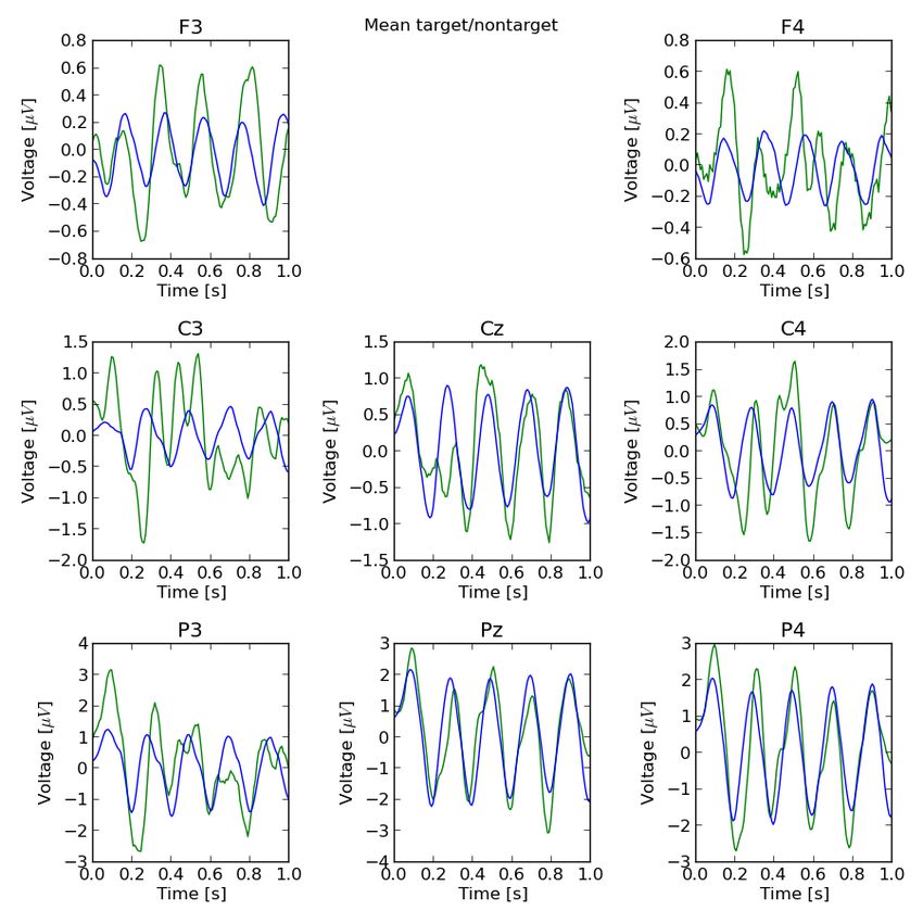
Abstract (English)
Brain-computer interfaces (BCI) provide the ability to control computer without any activity
in the peripheral nervous system. Although it has been more then two decades since the first
interface was built, their speed is still insufficiently low. This led to recent trends in research
community to build hybrid BCI.
The goal of this thesis was to construct a hybrid interface based upon P300 BCI paradigm and
eye tracker built from off-the-shelf parts. Resulting system showed a very promising bit rate
of 86.45 bits/min. Apart from construction of the specialized eye tracking hardware, the main
results of this study are due to the data analysis methods designed especially for this system.
They rely mostly on Common Spatial Pattern (CSP) filter, Fisher’s Linear Discriminant analysis
(FLD) and filters in time and frequency domains. Decisions made by the interface are based
upon probability values returned from individual modules.

                                    Key words (English)
Hybrid brain-computer interface, P300, Eye tracker, OpenBCI, Python, Brain-computer inter-
face, CSP, FDA

                                     Acknowledgements
First of all, I would like to gratefully acknowledge the supervision of my advisor, dr Rafał Kuś,
who has been abundantly helpful and patiently guided me through all processes of this work.
Moreover, I am very grateful to my individual course of study tutor dr hab. Piotr Durka for his
guidance during all my years at the University.
I would like to thank all those associated with the Biomedical Physics Division, especially dr
hab. Jarosław Żygierewicz and dr hab. Piotr Suffczyński, for their general assistance.
Last, but not least, I am grateful to my parents for their support and understanding.

                                                2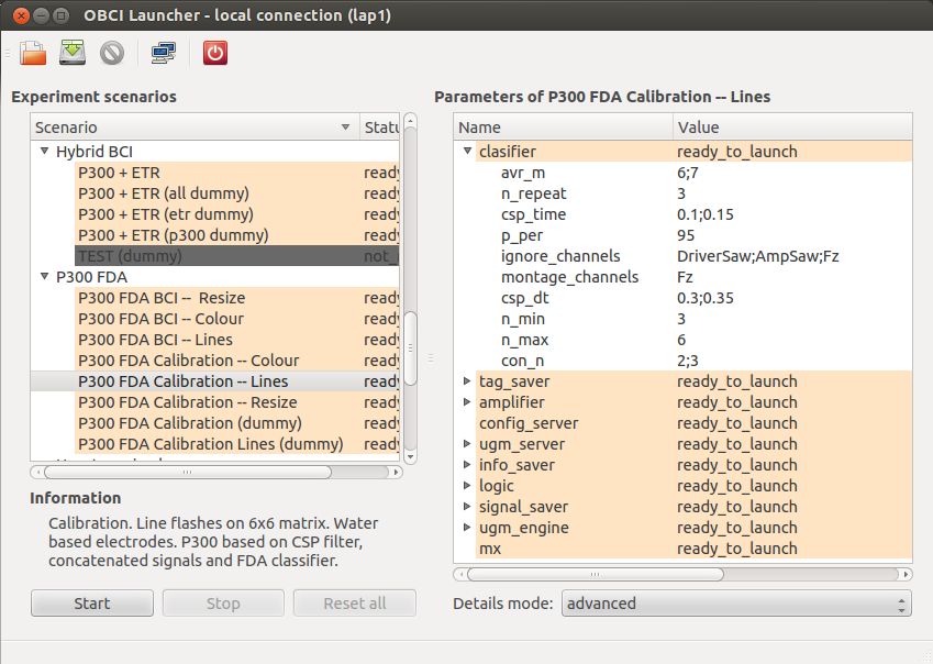
Contents

1. The Aim of this work . . . . . . . . . . . . . . . . . . . . . . . . . . . . . . . . . . .           4

2. Event-related potentials . . . . . . . . . . . . . . . . . . . . . . . . . . . . . . . . .           5

3. Methods for P300 analysis . . . . . . . . . . . . . . . . . . . . . . . . . . . . . . .              7
   3.1. Common Spatial Pattern         . . . . . . . . . . . . . . . . . . . . . . . . . . . . . . .    7
   3.2. Fisher’s Linear Discriminant . . . . . . . . . . . . . . . . . . . . . . . . . . . . . .       13
   3.3. Signal processing . . . . . . . . . . . . . . . . . . . . . . . . . . . . . . . . . . . .      14
   3.4. Selection of optimal parameters . . . . . . . . . . . . . . . . . . . . . . . . . . . .        15

4. P300 paradigm interface . . . . . . . . . . . . . . . . . . . . . . . . . . . . . . . . .           18
   4.1. Implementation . . . . . . . . . . . . . . . . . . . . . . . . . . . . . . . . . . . . .       18
   4.2. P300 calibration . . . . . . . . . . . . . . . . . . . . . . . . . . . . . . . . . . . .       20
   4.3. Speller application . . . . . . . . . . . . . . . . . . . . . . . . . . . . . . . . . . .      20

5. Eye tracker . . . . . . . . . . . . . . . . . . . . . . . . . . . . . . . . . . . . . . . . .       22
   5.1. The eye tracker built for this thesis . . . . . . . . . . . . . . . . . . . . . . . . . .      22
   5.2. Pupil detection . . . . . . . . . . . . . . . . . . . . . . . . . . . . . . . . . . . . .      22
   5.3. Cursor movement . . . . . . . . . . . . . . . . . . . . . . . . . . . . . . . . . . . .        23

6. Combination of P300 and eye tracking interfaces . . . . . . . . . . . . . . . . .                   25
   6.1. The P300 interface . . . . . . . . . . . . . . . . . . . . . . . . . . . . . . . . . . .       25
   6.2. The eye tracker interface . . . . . . . . . . . . . . . . . . . . . . . . . . . . . . . .      26
   6.3. The hybrid interface . . . . . . . . . . . . . . . . . . . . . . . . . . . . . . . . . .       26

7. Results . . . . . . . . . . . . . . . . . . . . . . . . . . . . . . . . . . . . . . . . . . . .     28
   7.1. Calibration and individual tests . . . . . . . . . . . . . . . . . . . . . . . . . . . .       28
   7.2. Both methods operating in parallel . . . . . . . . . . . . . . . . . . . . . . . . . .         29

8. Discussion . . . . . . . . . . . . . . . . . . . . . . . . . . . . . . . . . . . . . . . . . .      34

9. Summary . . . . . . . . . . . . . . . . . . . . . . . . . . . . . . . . . . . . . . . . . .         37

                                                   3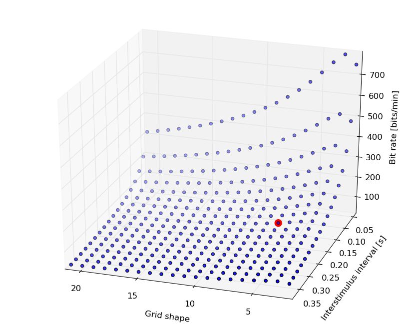
Chapter 1

The Aim of this work

Brain-computer interface (BCI) is a system which allows users to control the computer without
any muscles activity. According to the definition from the review of the first international BCI
technology meeting: “A brain–computer interface is a communication system that does not
depend on the brain’s normal output pathways of peripheral nerves and muscles” [1]. These
interfaces are divided into two categories: dependent and independent [2]. The dependent BCI
requires at least partially peripheral activity, but it interprets only the brain activity, whereas
independent one demands only brain’s normal activity.
BCIs have been under development since 1988 [3, 4, 5, 6, 7, 8], nevertheless, the progress in the
bit rate and stability of the communication is disappointingly slow. Therefore, recently, many
scientists turned their attention towards hybrid BCI (hBCI), which is composed of two BCIs,
or at least one BCI and another system [9]. As an example of such interfaces one can con-
sider BCI based on steady-state visual evoked potentials (SSVEP) paradigm and event-related
desynchronization/synchronization (ERD/ERS) paradigm [10] or P300 and SSVEP paradigms
[11]. Recently, authors of an article [12] pointed the need for creating a hybrid BCIs including
the P300 paradigm, which are thought to be promising. Moreover, according to a paper [13], a
combination of BCI with existing assistive technologies (AT) would provide more practical use
for disable people.
While the techniques of recording of the brain electrical activity from the surface of the head
(Electroencephalography, EEG) are very well developed over the last 90 years [14], the major
challenge remains in the methods used for extraction of relevant features, that is data analysis.
The aim of this work was to develop robust and effective methods of data analysis for a hybrid
BCI consisting of P300 paradigm and assistive technology — an eye tracker. As a result, a
complete system was build based on OpenBCI software and cheap eye tracker build from off-
the-shelf components. The P300 module employs adaptive statistical approach to the minimal
number of repetition, while the eye tracker provides selection based on spatially distributed
heatmaps.

                                                4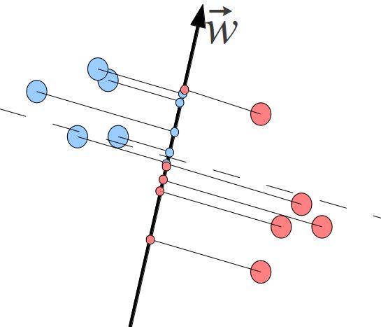
Chapter 2

Event-related potentials

An event-related potential (ERP) is defined as “Scalp-recorded neural activity that is generated
in a given neuroanatomical module when a specific computational operation is performed“ [15].
It can be either endogenous, when it is dependent on internal factors, or exogenous, if it is
elicited by outer cue, such as flash of light. The amplitude of these components is very low and
rarely exceeds few microvolts.
The basic method of extracting ERPs from EEG is averaging the signals time-locked to the
event. This is based on the assumption that response evoked by the stimulus r(t) is always the
same, however, it is covert with normal brain activity which is trial-independent and can be
described as zero mean noise n(t). Thus, after k-th stimulus one can measure:

                                         xk (t) = r(t) + nk (t).

After averaging over all trials

                         N                               N                               N
                                    !                                   !
                     1   X                1              X                             1 X
             x̄(t) =           xk (t)   =     N r(t) +         nk (t)       = r(t) +       nk (t)
                     N                    N                                            N
                         k=1                             k=1                             k=1

Hence, the more trials (N ) the better evoked waveform is visible. Normally, at least few dozens
have to be obtained.
Plot presented in Figure 2.1 is an idealised example of averaged over trials time-locked brain
response to the stimuli. The graph was drawn with negative voltage upwards, which is common
presentation of ERP waveforms in neuroscience. Usually, voltage deflections (components) are
labelled with a letter, which denotes its sign (P for positive and N for negative), and a number
indicating either ordinal position in waveform (for example N1) or latency in milliseconds after
the stimulus (like N100).
The largest ERP component is P300, which peak is about 300 ms after a stimulus. One of the
first, still the most popular and robust BCIs are based on this waveform [3]. The P300 can
be generated during the oddball paradigm, in which a subject is presented with a sequence of
events. These events can be categorized into two groups and one of which is rarely displayed.

                                                   5
Figure 2.1: Some of the ERP components. Stimulus onset at time 0 s. Note that voltage is
plotted negative upwards. Figure obtained from [16] under CC licence.

Figure 2.2: Waveform obtained from experimental data with two ERP components marked.
Stimulus onset at time 0 s.

In Figure 2.2 the response obtained from the experiment is presented. Both visible components,
N2 and P3, differ from the idealised waveform in amplitude and latency.

                                              6
Chapter 3

Methods for P300 analysis

Classical averaging technique mentioned in Chapter 2 is not sufficient for brain-computer inter-
face, as repetition of several dozens lasts too long. Advanced methods of extraction of the ERP
component, allowing for its detection only after a few instances, were designed in this work.
The proposed signal analysis methods use features of the potential like amplitude, latency and
shape. These features vary amongst people. Thus, it is important to perform for each user a
calibration procedure, while, after many repetitions of a target (expected stimulus) and non-
target (all other stimuli) the brain responses are collected and analysed. Based on the measured
signals the ERP detection, its feature extraction and classification can be performed.
Adequate EEG channels combination can emphasise feature’s visibility and its detection. Due to
the fact that ERP location varies between people the estimation of the optimal channel montage
which amplifies the event-related potential is non-trivial problem. The procedure of automatic
adjustment of channels montage, implemented in this work, is called Common Spatial Pattern
(CSP) and is described in section 3.1.
Classification procedure of analysed signals is described in Section 3.2. All steps of signal
processing are presented in Section 3.3. The methodology of selecting the optimal parameters
for classifier is introduced in Section 3.4.

3.1. Common Spatial Pattern
Usage of spatial filter increases signal to noise ratio for detection a spatially distributed potential.
Common Spatial Pattern (CSP) is an example of such filter and it was first used in EEG analysis
as a detection method for abnormal signal components [17]. Since then it has been used with
success in many brain-computer interfaces, mainly in ERD/ERS paradigm [18].
The purpose of this method is to estimate EEG channel montage, optimal for discrimination
between two different conditions denoted as target (+) and non-target (−). The montage is
described by transformation matrix P , which projects signals as follows:

                                       ±
                                      XCSP (t) = P T · XR± (t) ,                                  (3.1)

                                                   7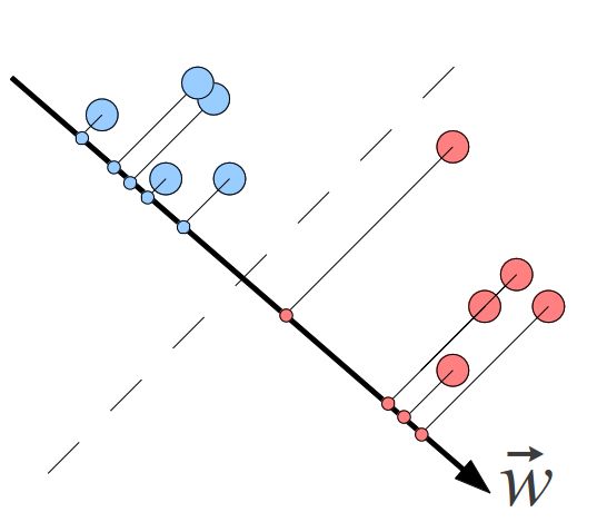
where X is EEG matrix and indexes R and CSP are respectively referred to raw signals and
signals after CSP transformation. The shape of X is C × N (X ∈ RC×N ), where C is number
of EEG channels and N holds for number of samples in each channel.
It is expected, that the obtained signals will fulfil the following conditions:
                   +            −
   1. The signals XCSP (t) and XCSP (t) are independent.

   2. There is no correlation between channels in each transformed signal.

   3. At least in one channel the variance of the transformed signals is maximized for targets
         and minimized for non-targets.

Covariance matrix of transformed signals, averaged over all trials, is given by:

                  ±      ±        ±
                                             T                        T
                 RCSP = XCSP (t) XCSP (t)         = P T XR+ (t) XR± (t) P = P T RR
                                                                                 ±
                                                                                   P,         (3.2)

       ±
where RR are covariance matrices of raw data averaged over all trials. Moreover, according to
                                +        −
conditions 1. and 2., matrices RCSP and RCSP should be diagonal.
The third condition can also be expressed as:

                                           +
                                          RCSP    −
                                               + RCSP = 1,                                    (3.3)

where 1 denotes identity matrix. Expanding formula (3.3) one can see that the diagonal values
(λ±            ±                                    +   −
  i refers to RCSP ) are bound with condition that λi +λi = 1. Thus, equations (3.2) represents
                                                                    +      −
the problem of simultaneous diagonalization of covariance matrices RR and RR . This can also
be represented with vectors as
                                          λ+
                                           i =p
                                                     +
                                              ~Ti · RR · p~i ,                              (3.4a)

                                          λ−
                                           i =p
                                                     −
                                              ~Ti · RR · p~i ,                              (3.4b)

where p~i are column vectors of matrix P . Considering ratio of equations (3.4a) and (3.4b) one
obtains:
                                                      +
                                           λ+
                                            i   p~Ti RR p~i
                                            − =    T  − ,                                     (3.5)
                                           λi   p~i RR p~i
which can also be transformed into

                                            +           −
                                           RR p~i = λi RR p~i ,                               (3.6)

                −
where λi = λ+
            i /λi . Equation (3.6) represents general form of eigenvalue problem, where eigen-
vectors p~i are interpreted as spatial filters. Thus, this method transforms raw signals into space
where signal variance best differentiates the two experimental conditions. The most discrimi-
native channels in CSP transformed signals are correlated to the largest eigenvalues due to Eq.
(3.3).
In case of the P300 paradigm the two experimental conditions can be distinguished. The first
one is presentation of the target stimulus, whereas any other stimuli is considered as the second

                                                    8
condition. It is expected that the information relevant to classification of the two conditions
is contained in a few transformed channels corresponding to the largest eigenvalues. This is
because the condition may affect a number of independent processes.
Example application of CSP
The impact of CSP filter on the EEG signals is presented in Figures 3.1, 3.2, 3.3 and 3.4. Figure
3.1 presents signals from individual electrodes averaged over all trials. Green lines represent
the signals recorded during target (“+”) condition, which should evoke a ERP component in a
window of range from 150 ms to 450 ms after stimulus onset, whereas red lines indicate reference
signals (non-target condition, “−“). Subtraction of both signals for all channels is displayed in
Figure 3.2. Figures 3.3 and 3.4 represent signals, average over all trials, composed of electrodes
which weight were respectively equal and determined by CSP filter. Top subplots include the
responses with and without desired features, whereas bottom subplots present subtraction of
these signals. Although in top of frame of Figure 3.3 it is hard to distinguish a difference between
target and non-target condition, it is easy detect the deflection about 0.2 s after stimulus onset in
their subtraction. After the CSP filter (Fig. 3.4) one can notice the difference in both subplots.
Moreover, the peak-to-peak value of the feature in subtraction plots has increased twice, from
2 µV to 4 µV.
9Figure 3.1: Averaged responses for each channel with stimulus onset at time 0 s. Green and
blue lines denote respectively responses to target and non-target stimuli. Signals were high
pass filtered and smoothed by means of moving average. Plots correspond to topographical
electrode’s displacement.
10Figure 3.2: Subtraction of averaged target and non-target responses for each channel with
stimulus onset at time 0 s. Signals were high pass filtered and smoothed by means of moving
average. Plots correspond to topographical electrode’s displacement.
11Figure 3.3: Averaged responses obtained from mean of signals from all electrodes. In top figure,
green and blue lines denote respectively responses to target and non-target stimuli. Bottom plot
represents subtraction of non-target from target. Signals were high pass filtered and smoothed
by means of moving average.
Figure 3.4: Averaged responses obtained from electrodes combination expressed by the largest
CSP transformation matrix eigenvalue. In top figure, green and blue lines denote respectively
responses to target and non-target stimuli. Bottom plot represents subtraction of non-target
from target. Signals were high pass filtered and smoothed by means of moving average.
123.2. Fisher’s Linear Discriminant
The signals obtained in P300 paradigm can be divided into two categories: target (containing
P300 component) and non-target (any other signal). An algorithm which classifies signal, to
one of predefined groups, based on its features, is called a classifier.
Fisher’s Linear Discriminant analysis (FLD) is one of the most efficient methods for P300 com-
ponent extraction and classification [6, 19]. This method is simple to calculate and provides
robust classification. Essence of this technique is to find a linear combination of features which
best discriminates both classes. To do so, one attempts to find a hyperplane in N–dimensional
hyperspace, that fully separates these categories.
In order to briefly explain how this method works a sample classification on 2 datasets of two
dimensional values is presented. For such case a separating hyperplane is a line, which maximizes
the distance, of the two groups, measured along the direction perpendicular to the line (Fig.
3.5).
(a) Good separation of two datasets. (b) Poor separation.
Figure 3.5: The graphs present basic concept of FLD method. Dots are grouped depending
on their colour. Dashed line represents separating hyperplane, whereas w
~ is its normal vector.
Projections are routed with continuous lines from dots onto the normal vector.
The dividing hyperplane is estimated under the condition of maximization of the ratio of the
variance between classes to the variance within classes. This can be expressed with an equation:
~ T SB w
w ~
J (w) = T
, (3.7)
w
~ Sw w ~
where SB and SW are respectively scatter matrices between classes and within classes. Vector w
~
is a projection direction, which best separates both groups. Scatter matrices can be estimated
13by covariance matrix, that is:
~ )T ,
P
SB = c (~
µc −µ
~ ) · (~
µc − µ
(3.8)
~ c )T ,
P P
SW = c xi − µ
i∈c (~ ~ c ) · (~xi − µ
where:
1 P
µ
~c = Nc i∈c ~
xi ,
1 P P
(3.9)
µ
~= N c i∈c ~
xi ,
c ∈ {+, −}.
In equations (3.9) Nc is the number of trials for a single class c, N is the total number of all
trials (N = N+ + N− ) and ~xi is a single data point.
One can shift origin so that scatter matrices are calculated in respect to one of the groups. This
procedure simplifies the expression for variance between classes to:
0
SB µ+ − µ
= (~ ~ − ) · (~ ~ − )T ,
µ+ − µ (3.10)
~ → αw;
Equation (3.7) is invariant with respect to rescaling of vectors w ~ thus if one assumes that
~ T SW w
the denominator satisfies w ~ = 1, then the maximization of the equation (3.7) requires the
~ T SB w,
minimization of the formula −w ~ what can be described in lagrangian formalism as
~ T SB w ~ T SW w
L = −w ~ +λ w ~ −1 . (3.11)
It can be shown [20] that formula (3.11) is maximized with vector:
~ = (Σ+ + Σ− )−1 (~
w µ+ − µ
~ −) , (3.12)
where Σ+/− are covariance matrices of signals recorded under target and non-target conditions.
Each new dataset (~s) is classified based on the result from projection onto the vector w
~
~ · ~s − c,
d=w (3.13)
where variable c is a threshold value and is substituted with 95th percentile score of non-target
distribution. Result of Eq. (3.13) is called d-value and it indicates how well new data fits into
the target class.
3.3. Signal processing
The calibration procedure is performed in following steps:
1. EEG signal consisting of C channels sampled with frequency S is converted into two
datasets of target and non-target respectively shaped into T × C × S and N T × C × S
matrices, where T and N T are the numbers of target and non-target stimuli.
142. Each signal is cropped to [csp time, csp time + csp dt] range, where csp time is a time
value (in seconds) from stimulus onset and csp dt is a length (in seconds) of a window;
3. A CSP filter matrix P is obtained, accordingly to Eq. (3.6), and its eigenvectors are sorted
in decreasing order of eigenvalues;
4. All signals are filtered with 2nd order 1.5 Hz cutoff high pass Butterworth filter and
averaged with avr m + 1 samples long window by means of moving average, where avr m
is the number of features to be extracted from analysed window;
5. Produced signals are downsampled to avr m evenly distributed points;
6. First con n eigenvectors of matrix P are consecutively concatenated;
7. Estimated FLD classifier’s hyperplane w
~ vector and c threshold are stored.
The set of variables from this procedure is denoted as G = {csp time, csp dt, avr m, con n}.
Signal processing is performed for each combination of parameters. The set which denotes the
best overall result is used in online analysis.
3.4. Selection of optimal parameters
For a given set of parameters G, described in section 3.3, a collection of d-values (Eq. (3.13)) for
targets {dT } and for non-targets {dN T } are obtained. For these values the Mann-Whitney U
statistics is computed using the function from SciPy statistical package. The set of parameters
which yields the most separated sets of {dT } and {dN T } is indicated by the lowest value of the
statistics U.
Additional control over the parameters (G) is provided by two types of plots. The first one,
exemplified in Figure 3.6, represents plots of averaged signals of elicited responses. Respectively
top and bottom rows correspond to the target and non-target stimulation. Curves in red indicate
single response after every cue, whereas green is an averaged signal over all stimuli. First column
represents signals computed by combining all channels with the same weights (simple mean),
where the second, third and fourth are evaluated with weights from CSP eigenvectors respectively
to the first, second and third largest eigenvalues.
The second type of figures displays distributions of d-values (Eq. (3.13)) for the targets and non-
targets. In Figure 3.7 the top left subplot represents histogram of the non-target distribution,
whereas the top right represents the target distribution. Vertical red lines indicate the average
values for given plot. The zero value is placed in 95th percentile of the non-target distribution.
Comparison of both distributions is presented in bottom subplot.
Both plots can be used to verify the selection of:
time limits for CSP computations (time interval when the average shows pronounced
deflections in targets),
15Figure 3.6: Plots obtained after calibration procedure. Rows present responses for target (top)
and non-target (bottom) stimulus. Red lines are related to a single trials, while green are
averaged responses. The first from left column displays simple mean signals from all electrodes.
The second, third and forth are related respectively to the first, second and third CSP eigenvector
combinations.
Figure 3.7: Histograms of the target and non-target values. Top left and top right histograms
represent respectively distributions of d-values for non-target and target cases. Red vertical lines
indicate mean values. The bottom subplot shows both distributions overlaid.
16 the number of CSP transformed channels to be used — it can be visually assessed in how
many of such channels there is a significant difference between targets and non-targets.
17Chapter 4
P300 paradigm interface
4.1. Implementation
Methods designed and discussed in this work were implemented in Python Programming Lan-
guage. Numerical analysis were done using NumPy (http://numpy.scipy.org/) and SciPy
(http://www.scipy.org/) packages. All plots were made with use of Matplotlib (http://
matplotlib.sourceforge.net/) package.
Implemented interface is a part of the OpenBCI [21] system, which is an open source architecture
for brain-computer interfaces. It is free to use and can be downloaded from git repository
http://escher.fuw.edu.pl/git/openbci/. Contributions to OpenBCI from this work are
stored in path interfaces/hybrid/p300etr relative to the main directory.
The system is equipped with a program called obci gui, which provides the user with control
over all modules, allowing to start/stop execution of any program, or change it’s parameters. In
Figure 4.1 a view on classifier’s options for P300 Calibration module are presented.
The EEG signals, sampled at 128 Hz frequency, are recorded from F3, F4, C3, Cz, C4, P3, Pz
and P4 electrodes with reference to Fz electrode (Fig. 4.2) according to the international 10–20
standard system. Each signal is filtered with high pass filter and smoothed by moving average
of a window length dependent on G parameter set (described in section 3.3).
The P300 interface designed within this work is divided into two modules:
P300 calibration,
Speller application,
Both modules use the same speller matrix for stimuli, which consists of 6 rows and 6 columns
of evenly distributed rectangles with symbols placed in their centres (see Figure 4.3a). The
top grey box indicates a space where selected characters are displayed. The ERP responses are
elicited by randomly lighting up line of blocks for 100 ms followed with 100 ms of pause. An
example of stimulus is presented in Figure 4.3b.
18Figure 4.1: A view of a obci gui software, which is a graphical user interface designed for
maintaining BCI scenarios.
Figure 4.2: Position of EEG electrodes on the surface of the head according to the International
10–20 standard. The electrodes marked with red colour were used for recording of EEG signals,
whereas blue one indicates reference electrode.
19(a) Without any stimuli. (b) The P300 stimulus as highlight of 3rd column.
Figure 4.3: A speller grid of 36 symbols used in the P300 interface. All lines, columns and rows,
highlight sequentially with intervals of 200 ms. During the calibration user has to focus his/her
attention on predefined character for 10 trials separated by 5 s long break. In a single trial, each
line highlights in random order from 8 to 10 times. In speller application mode one can select
any symbol by concentrating attention on it.
4.2. P300 calibration
Before a user can control computer with the P300 interface it has to be calibrated. User is
asked to focus his/her attention on a single character and count in thoughts how many times
it was elicited. A stimulus is a change of line’s background colour from black (#000000) to red
(#E42525). Each blink lasts for 100 ms and is followed by a break of the same length. After
10 trials, where each one includes from 72 to 84 stimuli flickerings, system tries to determine
the best G parameters set. Signals recorded during the calibration are used for selection of the
optimal CSP (sec. 3.1) and FDA parameters (sec. 3.2).
4.3. Speller application
General scheme of operation of the P300 interface is presented in Fig. 4.4. The amplifier records
EEG signals, which are analysed and, based on their the output, a decision is made. Feedback
is provided by displaying a character on the speller matrix.
P300 P300 Speller
EEG Amplifier Feedback
Analysis Decision matrix
Figure 4.4: Block scheme of the P300 interface.
Speller is based upon the grid presented in Figure 4.3. User selects symbol by concentrating
his/her attention on it. P300 potential is evoked by highlighting rows and columns in random
order for 100 ms with intervals lasting for 100 ms in between. After each stimulus, one second
of EEG signal is passed to the signal processing module, as mentioned in section 3.3. Obtained
20result is projected onto vector w
~ (perpendicular to FLD hyperplane, sec. 3.2) producing the
d-value (Eq. 3.13).
When each field highlights at least nM in times, program tries to find out to which field, defined
by row and column crossing, P300 potential can be associated. Decision is made on averaged
d-value a row and a column in which intersection the field is located
[c] [r]
[cr] di + di
di = (4.1)
2
based on no more than nLast line blinks after previous decision
n=N
1 X [cr]
d[cr] = di . (4.2)
N
n=0
The above procedure produces a 6 × 6 shaped matrix D of d-values. For each score a percentile
is calculated from non-target distribution. If there is only one d[cr] value for which this fraction
is greater than 95%, algorithm a makes decision corresponding to that field. More than one or
no, significant differences evoke another sequence of stimuli. After nM ax unsuccessful attempts
algorithm forces analysis module to make a decision by choosing the one with the highest score.
For example, setting nM ax = 1000 and nLast = 10 should result in a system, that would
minimize false positive rate (FP) detection during a period, when the user does not use the
interface. When a decision is made, the corresponding rectangle lights up in green for a second,
providing a visual feedback to the user.
21Chapter 5
Eye tracker
The eye tracker is a device which measures the movement of the eye [22]. In general, eye trackers
can be divided into two types [23]: either those that determine the position of the eye relative
to the head, or those that measure the eye’s orientation in space — the “point of regard“.
Devices belong to the second category, are commonly called gaze trackers, as they provide the
information about the point of gaze. The application of eye trackers varies widely across all
disciplines, these include: research tool in cognitive or advertising studies, a game controller or
an assistive technology for disable people.
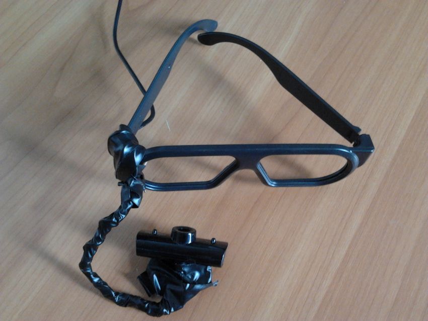
5.1. The eye tracker built for this thesis
The eye tracker, which was built by the author of this thesis and used in all experiments within
this work, is presented in Figure 5.1. The device consists of a webcamera supported on thick
copper wire, which is attached to plastic sunglasses holder. To preserve constant eye illumination,
that also does not annoy user, an infra red light was used. Two IR light emitting diodes (IR
LED) are placed on both sides of the camera and an IR filter is embedded between camera’s
lenses. Intensity of used LEDs is 20 mW/sr when powered with 20 mA current. Their peak
wavelength is λ = 940 nm with spectral bandwidth of ∆λ = 50 nm. The inspiration for building
such an eye tracker were instructions found on the internet at [24].
The main advantage of this eye tracker is it’s relative low cost, which is below $ 50. In contrast,
commercially available solutions, with prices above $ 6,000[25], are currently beyond reach of
average household.
5.2. Pupil detection
Conversion of an eye movement signal into cursor movement is made with EyeWriter application
obtained from the Internet (http://code.google.com/p/eyewriter/). It’s configuration window
is displayed in Figure 5.2. Purpose of image analysis is to find centre of pupil which is done in
following steps:
1. Circled area of image, containing pupil, is cropped.
22Figure 5.1: The eye tracker used in experiment.
2. New image is adjusted with brightness and contrast.
3. Pixels with values below set threshold are replaced with white pixels and the rest is turned
black.
4. White pixels are dilated into single blob to which ellipse is fitted.
5.3. Cursor movement
When pupil is detected one can proceed to software calibration, which will assign cursor’s co-
ordinates to pupil’s position. This procedure is done by displaying sequentially dots in crossing
of a grid presented in Figure 5.3. User’s task is to gaze at centre of each dot until it changes
position. It is critical not to move the head at any time during the calibration as it will result
in inaccuracy of cursor’s position. After calibration procedure green dot appears at place where
user is currently looking.
23Figure 5.2: EyeWriter configuration screen. Top left panel displays raw camera image. Top
right screen shows adjusted and circled cropped video. Bottom left view includes converted top
right image into binary format with set threshold value. Bottom right grey image indicates
pupil’s centre and an ellipse fitted to it’s contour.
Figure 5.3: EyeWriter calibration screen. In calibration mode program assigns cursor’s coordi-
nates to pupil’s position. A dot, which should attract one’s attention, travels from bottom left
to top left corner via each grid’s crossing, where it stops for a second. After 0.75 s from the
beginning of the break it turns red for 0.25 s, which means that it records current user’s eye
position.
24Chapter 6
Combination of P300 and eye
tracking interfaces
Both presented interfaces, the eye tracker and the P300, are designed to make independent
decisions. However, their simultaneous use requires validation of their predictions. Thus, both
modules pass the probabilities for each field of being a target to additional module, which
confronts them. Based on collective data, if only single option is significant, system produces a
decision. The block scheme for such solution is presented in Figure 6.1.
ETR ETR
Eye tracker
Analysis Probability
Hybrid BCI Speller
Feedback
Decision matrix
P300 P300
EEG Amplifier
Analysis Probability
Figure 6.1: Block scheme of created hybrid interface. Both modules, P300 and an eyetracker,
output probabilities which are confronted in Hybrid BCI Decision module and decision is passed
to speller matrix.
6.1. The P300 interface
After each epoch, which is denoted by single highlight of all possible lines, P300 analysis module
returns processed EEG signals, sc for columns and sr for rows, as described in section 3.3. Then,
these signals are projected onto the vector w
~ producing the d-values (Eq. 3.13). In a single trial,
each field is highlighted twice — in column block and in row block; thus, two signals can be
used to determine the current d-value for a stimulus. Since FLD classifier is a linear method,
these values can be easily obtained by averaging all d-values for lines to which they correspond,
25rather than averaging both signals and then projecting it:
d[cr] = 0.5w
~ · (~sc + ~sr ) = 0.5(w ~ · ~sr ) = 0.5(d[c] + d[r] ).
~ · ~sc + w (6.1)
As a result a matrix of projection values is returned. Each value can be described in terms of
probability as follows:
!
[cr]
[cr]
d[c] + d[r]
PP 300 = PerN T d = PerN T , (6.2)
2
where PerN T is a function which returns percentile score of non-target distribution for a given
argument. Thus, when a grid of 6 rows and 6 columns is considered, the probability matrix
Pp300 shape is 6 × 6.
6.2. The eye tracker interface
Coordinates of gaze ~r are sampled with constant frequency of 30 Hz and are expressed in screen’s
relative position, where (0,0) is the top left and (1,1) is the bottom right corner. Every fifth
sample, a mean value (h~ri) is calculated from last five samples and it’s distance (D) from the
centre of each possible stimulus rectangle is computed as:
q p
Dcr = |h~ri − R ~ cr |2 = (hxi − Xcr )2 + (hyi − Ycr )2 . (6.3)
~ cr = (Xcr , Ycr ) is the position of the field from column c and row r. To
In equation (6.3) R
emphasise fields located closely to current gaze coordinates, and to provide a rapid decrease
with distance, the function of probability is considered as a gaussian function, that is:
[cr] 2
PET R = exp −λDcr · 100%, (6.4)
where λ is a positive normalization parameter. It’s value is determined by the condition, that
the probability in distance of two nearest fields should decrease from 100% to 50%, which is
fulfilled when λ is as follows:
λ = log(2)N, (6.5)
where N is the number of rows (or columns, in a square grid) and log expresses natural loga-
rithmic function. The outcome probability function is displayed in Figure 6.2.
6.3. The hybrid interface
The general form of cumulative probability from both interfaces can be described with formula
[cr] [cr] [cr]
Ptot = α · PP300 + (1 − α) · PETR , (6.6)
[cr] [cr]
where PP300 and PETR are respectively described by equations (6.2) and (6.4). Presented in Eq.
[cr]
(6.6) parameter α (α ∈ [0, 1]) denotes the quantitative composition of the PP300 into outcome
probability. Thus, if α = 0, then total probability matrix depends only on eye tracking interface.
26Figure 6.2: Colour map of probability function, when gaze is in the centre of the field in the
third row and third column.
For purpose of this work both modules were taken into account with same weights, ergo α
parameter was set to be 1/2. This presents the overall outcome probability as follows
[cr] 1 [cr] 1 [cr]
Ptot = ·P + ·P . (6.7)
2 P300 2 ETR
After each P300 epoch the system makes an attempt to deduce if user is trying to select any
symbol. Positive decision is made when there is only one score above 90%. If there is none, or
more than one, then the system waits until the end of another epoch.
It is possible that one of the modules, either eye tracking interface, or P300 paradigm, may
perform better. For such case an additional condition for making decisions was formulated. If
a single score from PP300 matrix is greater then 90% and all values in PETR are less then 65%
then a symbol is selected according to P300 module. Likewise, if there is no significant response
for ERP target stimulus (< 65%), but distinctive score from PETR probability matrix (> 90%),
then the field is selected according to the outcome of the second method.
27Chapter 7
Results
Proposed system was tested by a single male subject without any disabilities. EEG signal
was collected using TMSI Porti7 EEG amplifier with 128 Hz sampling frequency. Water based
electrodes were placed at 10–20 EEG standard in F3, Fz, F4, C3, Cz, C4, P3, Pz and P4 with
Fz being reference electrode (same as on Fig. 4.2). As a ground for amplifier a disposable ECG
sticker electrode was placed at degreased skin over clavicle bone.
7.1. Calibration and individual tests
P300 module
Whole interface calibration proceeded in two steps, for each module separately. Firstly, P300
module was calibrated as mentioned in section 4.2 on page 20. To verify obtained results user
had to focus his attention on letter “H” which is positioned in the second row and the second
column. Test lasted until system had made 9 decisions. Gathered results are plotted in Figures
7.2 and 7.3.
First colour map (Fig. 7.2) represents progress of the probability matrices produced in a 7th
trial. Ordinal number of each plot corresponds to the number of each line highlights. One can
see, that the second row and the second column are distinctive in each graph.
Figure 7.3 presents cumulative probability after 6 flashes of each line (12 flashes for each field)
for each trial. System correctly chose letter “H” 8 out of 9 times. Only in the second trial a
wrong decision was made, with only slight difference.
Eye tracking module
To examine the reliability of the eye tracker, user also tested the respective interface. After
successful calibration, as presented in section 5.3, user’s task was to concentrate gaze at letter
“H” for 15 consecutive decisions. As seen in Figure 7.4, which presents probabilities that given
field will be chosen, there is 100% accuracy.
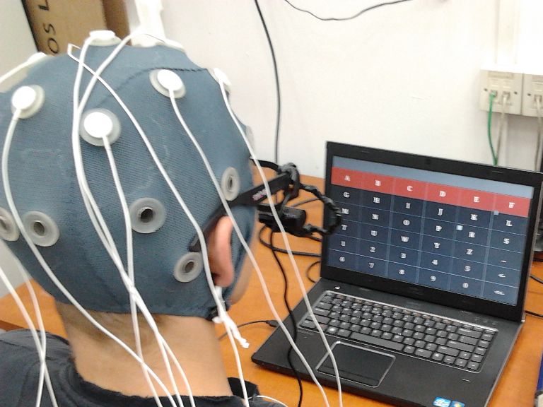
28Figure 7.1: User controlling the hybrid BCI interface. It consists of a professional EEG system
and eye tracker, built from off-the-shelf components.
7.2. Both methods operating in parallel
To test hybrid interface user’s task was to write a sentence “HYBRID BCI”. All lines had to be
highlighted at least once, before decision could be made. Whole test was repeated 5 times in a
row for better credibility. Colour maps presented in Figures 7.5, 7.6 and 7.7 were created from
first test’s data and they present probability matrices prior to decision, respectively for p300
module, eye tracking module and hybrid interface. Summary results from all tests are presented
in Table 7.1.
The performance of the interface can be measured by the Information Transfer Rate (ITR) [26]
as
A 1−p
B (p, N, T ) = p log2 (p) + (1 − p) log2 + log2 (N ) , (7.1)
T N −1
where p is accuracy denoted as a ratio of number of true positive selection to number of all made
decision (A), N is number of all possible different decisions and T is the time duration in which
decisions were made.
Considering 100% accuracy (p = 1) and square grid of n columns/rows of possible options
(N = n2 ), then Eq. 7.1 transforms into
A A
B (n, T ) = log2 n2 = 2 log2 n. (7.2)
T T
Maximum bit rate can be obtained when decision is made after single epoch, that is all line
29Figure 7.2: Colour maps obtained from single test trial of P300 module. User’s task was to
focus his/her attention on field in second row and second column. Plots represent progress of
probability matrices. Values are presented in percentage. Plot’s number, where top-left is one
and bottom-right is 6, corresponds to number of blink for each line.
highlight at least once. This denotes time duration as T = 2n∆t, where ∆t is the time inter-
val between consecutive stimulus, also called interstimulus interval (ISI). Thus, the maximum
theoretical bit rate is:
log2 n2
log2 (n)
Bmax (n, T ) = = . (7.3)
2n∆t n∆t
The maximum possible bit rate of presented interface (n = 6 and ∆t = 0.2 s) is 2.15 bits/s
or 129.25 bits/min. However, to estimate the actual information transfer rate, one also has to
take into account a feedback pause, when selected character is displayed. The experiment was
conducted with 1 s pause, which results in decreasing the maximum speed to 1.52 bits/s (91.23
bits/min). In total, it took 179.4 seconds to write 50 letters at 100% accuracy, providing an
average of 3.588 seconds per character and bit rate of 1.44 bits/s or 86.45 bits/min.
30Figure 7.3: Colour maps obtained from usage of P300 module. Each plot represents probability
matrices for fields to be target stimuli. Values are represented in percentage. User’s task was to
focus attention 9 times on field in crossing of second row and second column.
Table 7.1: Summary results from all tests.
Test No. Total No. of epochs Total time [s] Accuracy [%]
1. 12 37.8 100
2. 11 35.4 100
3. 13 40.2 100
4. 10 33.0 100
5. 10 33.0 100
Mean 11.2 35.88 100
31Figure 7.4: Colour maps obtained from tests of eye tracking module. User’s task was to con-
centrate gaze at second row and second column. Colours represent probability that the field is
target. All decision were correct.
Figure 7.5: Colour map of P300 probability produced after single stimulus of all rows and
columns. Each plot corresponds to different character.
32Figure 7.6: Colour map of eye tracker module probabilities produced after single stimulus of all
rows and columns. Each plot corresponds to different character.
Figure 7.7: Probability of field being target represented in colour maps. Each plot corresponds
to different character and was obtained after single stimulus of all rows and columns.
33Chapter 8
Discussion
In this work a method of data analysis for hybrid brain-computer interfaces is presented. The
interface consists of BCI paradigm called P300 and an eye tracking interface. To the best
author’s knowledge such combination has not yet been published.
Both modules, P300 and eye tracker, in each epoch return probability values for all possible
decisions. These probabilities are combined into the final decision in a way resembling a fuzzy
logic approach.
Calculated bit rate of the resulting system is estimated as 86.45 bits/min at 100% accuracy. The
obtained result cannot be compared to the bit rates of traditional and hybrid BCIs reported in
literature as they are based only on brain’s activities. Furthermore, information transfer rate
of the discussed interface, is based only on the one subject and more research are required for
better credibility. Current version is considered as a proof of concept, although, with great
potential for future developments and tests.
Presented interface can be easily adopted to all users. One can adjust impact of specific module
(P300 or eye tracker) by changing α parameter in total probability equation (Eq. (6.6)). The
subjects who control eye tracker well would set greater dependency on that module, whereas,
disable people without any eye control, or people who cannot fixate head in one position, would
benefit mostly from the P300 paradigm.
Although discussed interface provides very good results, a few changes should to improve the
overall performance:
The increase in general performance of the system could be achieved by embedding an EEG
artefact classification module, which would reject signals with too much noises. Potentials
induced by eye movement have hundred times larger amplitude than ERPs; thus, they
can modify these responses even after averaging over dozens of repetitions. Free from
noises signals would provide better estimation of component’s features and could improve
calibration process.
Modifications also can be made in reference to the process of selecting optimal parameters
34group G used in analysis. Currently, calculations are done on each set of parameters,
which is defined by user. This approach consumes much time and can result in accidental
omission of the best set. One of the solutions to this problem could be an implementation
method of the Mutual Information [27, 28]. This technique allows for determination of the
minimal number of the features which differentiate best two datasets.
The main disadvantage of the eye tracker interface is the lack of the algorithm to compen-
sate the head movement. This limits the number of users to such persons, who are able
to fixate their head position. An attempt to solve this issue using additional front-facing
camera is presented in Figure 8.2. Unfortunately, it was not possible to complete this
project within the time framework of this thesis.
The maximum bit rate (Eq. 7.3) of presented interface can also be increased by changing
properties of speller’s grid. Figure 8.1 shows change of bit rate in function of number of
columns/rows and interstimulus interval (ISI). The result obtained for discussed system is
emphasised with a red dot. Although, decreasing both values would benefit in increased
maximum theoretical transfer, this could lower the accuracy. Thus, tests are required to
determine the optimal shape and ISI value.
Another improvement to be considered is a feedback loop between eye tracking and P300
modules. If one assume that eye tracker works perfectly, then it could confirm or deny
decisions made by P300 module. Thus, one could assign the new signals to either tar-
get or non-target category, by eye tracker module, providing better estimations of both
distributions and allowing the P300 interface to adjust it’s parameters without additional
calibration. Likewise, if eye tracker performance would decrease, meaning that it’s vari-
ance would increase and both modules independent decision would differ significantly, then
an eye tracker’s calibration could be requested.
As discussed above, methods of data analysis and hardware presented in this study provide
satisfactory base for future developments and experiments.
35Figure 8.1: Bit rate dependency on grid’s shape and interstimulus interval (ISI) based on Eq.
(7.2). Presented interface’s speed is emphasised with red dot.
Figure 8.2: The first attempt to compensate for the head movements by using eye tracker with
additional front-facing camera. Reference LEDs, placed behind the screen, would be optimally
positioned in its corners, but this was not possible due to a narrow angle of the front-facing
camera.
36Chapter 9
Summary
The goal of this work was to present an approach to data analysis for hybrid BCI system. To
verify the operation of the algorithms designed for this thesis, a complete hybrid BCI system
was built based upon OpenBCI platform and a cheap eye tracker constructed from off-the-shelve
parts. The interface consists of BCI’s P300 paradigm and gaze tracking software. As presented
in Chapter 7, this interface is promising, as it provides bit rate of 86.45 bits/min with 100%
accuracy. However, interface’s performance was measured on a single subject; thus, for better
credibility, more tests should be conducted.
Proposed interface can be used by both disable patients and people without any disabilities.
Individuals who perform worse in one modality can adjust the system to their needs by changing
the impact of specific module on outcome decisions.
Designed interface is a part of OpenBCI system, which is free to use. It can be downloaded
from the git repository http://escher.fuw.edu.pl/git/openbci/. Modules created for this thesis
are stored in path interfaces/hybrid/p300etr relative to the main directory.
37Bibliography
[1] Jonathan R. Wolpaw, Niels Birbaumer, William J. Heetderks, Dennis J. McFarland,
P. Hunter Peckham, Gerwin Schalk, Emanuel Donchin, Louis A. Quatrano, Charles J.
Robinson, and Theresa M. Vaughan. Brain–computer interface technology: A review of the
first international meeting. IEEE Transactions on rehabilitation engineering, 8(2):164–173,
2000.
[2] J. R. Wolpaw, N. Birbaumer, D. J. McFarland, G. Pfurtscheller, and T. M. Vaughan.
Brain–computer interfaces for communication and control. Clinical Neurophysiology,
113:767–791, 2002.
[3] L. A. Farwell and E. Donchin. Talking off the top of your head: toward a mental prosthesis
utilizing event-related brain potentials. Electroencephalography and Clinical Neurophysiol-
ogy, 70(3):510–523, 1988.
[4] L. A. Miner, D. J. McFarland, and J. R. Wolpaw. Answering questions with an
electroencephalogram-based brain-computer interface. Arch Phys Med Rehabil, 79(9):1029–
1033, Sep 1998.
[5] Ming Cheng, Xiaorong Gao, Shangkai Gao, and Dingfeng Xu. Design and implementation
of a brain-computer interface with high transfer rates. 49(10):1181–1186, 2002.
[6] Ulrich Hoffmann, Jean-Marc Vesin, Touradj Ebrahimi, and Karin Diserens. An efficient
P300-based brain–computer interface for disabled subjects. Journal of Neuroscience Meth-
ods, 167(1):115–125, 2008.
[7] Dawid Laszuk. Implementacja paradygmatu P300 w systemie OpenBCI, 2011. Bachelor’s
thesis.
[8] P. J. Durka, R. Kuś, P. Milanowski, J. Żygierewicz, M. Michalska, M. Łabęcki, T. Spustek,
D. Laszuk, A. Duszyk, and M. Kruszyński. User-centered design of brain-computer inter-
faces: OpenBCI.pl and BCI Appliance. volume 3, 2012.
[9] B Z Allison, R Leeb, C Brunner, G R Müller-Putz, G Bauernfeind, J W Kelly, and C Neu-
per. Toward smarter BCIs: extending BCIs through hybridization and intelligent control.
Journal of Neural Engineering, 9(1):013001, 2012.
38[10] Brendan Z. Allison, Clemens Brunner, Christof Altstätter, Isabella C. Wagner, Sebastian
Grissmann, and Christa Neuper. A hybrid ERD/SSVEP BCI for continuous simultaneous
two dimensional cursor control. Journal of Neuroscience Methods, 209:299–307, 2012.
[11] R. C. Panicker, S. Puthusserypady, and Y. Sun. An asynchronous P300 BCI with SSVEP-
based control state detection. IEEE Trans Biomed Eng, 58(6):1781–1788, Jun 2011.
[12] Reza Fazel-Rezai, Brendan Z. Allison, Christoph Guger, Eric W. Sellers, Sonja C. Kleih,
and Andrea Kübler. P300 brain computer interface: current challenges and emerging trends.
Frontiers in Neuroengineering, 5(00014), 2012.
[13] J. del R. Millán, R. Rupp, G. Müeller-Putz, R. Murray-Smith, C. Giugliemma, M. Tanger-
mann, C. Vidaurre, F. Cincotti, A. Kübler, R. Leeb, Ch. Neuper, K. R. Müeller, and
D. Mattia. Combining brain-computer interfaces and assistive technologies: State-of-the-
art and challenges. Frontiers in Neuroscience, 4(00161), 2010.
[14] H. Berger. Über das elektroenkephalogramm des menschen. Arch. Psychiatr., 87:527–570,
1929.
[15] Steven J. Luck. An Introduction to the Event-Related Potential Technique. The MIT Press.,
2005.
[16] Wikipedia society. Components of ERP. http://en.wikipedia.org/wiki/File:ComponentsofERP.svg,
August 2012.
[17] Z. J. Koles. The quantitative extraction and topographic mapping of the abnormal com-
ponents in the clinical EEG. Electroencephalography Clinical Neurophysiology, 79:440–447,
1991.
[18] H. Ramoser, J. Müller-Gerking, and G. Pfurtscheller. Optimal spatial filtering of single
trial EEG during imagined hand movement. IEEE transactions on rehabilitation engineer-
ing: a publication of the IEEE Engineering in Medicine and Biology Society, 8(4):441–446,
December 2000.
[19] Dean J. Krusienski, Eric W. Sellers, Francois Cabestaing, Sabri Bayoudh, Dennis J. Mc-
Farland, Theresa M. Vaughan, and Jonathan R. Wolpaw. A comparison of classification
techniques for the P300 Speller. Journal of neural engineering, 20(3):299—-305, 2006.
[20] Keinosuke Fukunaga. Introduction to Statistical Pattern Recognition. Academic Press, San
Diego, CA, USA, 2nd edition edition, 1990.
[21] University of Warsaw Biomedical Physics Division, Faculty of Physics. OpenBCI system.
http://bci.fuw.edu.pl/, August 2012.
39[22] Andrew Duchowski. Eye Tracking Methodology. Springer, 530 Walnut Street, Philadelphia,
Pennsylvania 19106-3621 USA, second edition, 2007.
[23] Laurence Young and David Sheena. Survey of eye movement recording methods. Behavior
Research Methods, 7:397–429, 1975. 10.3758/BF03201553.
[24] The EyeWriter Development Team. The EyeWriter. http://www.instructables.com/
id/The-EyeWriter/, July 2012.
[25] Tobii Technology. Eye tracking and eye control for research, communication and integration.
http://www.tobii.com/, July 2012.
[26] J.R. Wolpaw, D.J. McFarland, and T.M. Vaughan. Brain-computer interface research at
the Wadsworth center. IEEE Transactions Rehabilitation Engineering, 8:222–226, June
2000.
[27] C. E. Shannon. A mathematical theory of communication. The Bell Systems Technical
Journal, 27:379–423, 623–656, 1948.
[28] Thomas M. Cover and Joy A. Thomas. Elements of information theory. Wiley-Interscience,
New York, NY, USA, 1991.
40You can also read