Geodesics in Heat: A New Approach to Computing Distance Based on Heat Flow
←
→
Page content transcription
If your browser does not render page correctly, please read the page content below
Geodesics in Heat:
A New Approach to Computing Distance Based on Heat Flow
KEENAN CRANE
Caltech
CLARISSE WEISCHEDEL, MAX WARDETZKY
University of Göttingen

We introduce the heat method for computing the geodesic distance to a
specified subset (e.g., point or curve) of a given domain. The heat method is
robust, efficient, and simple to implement since it is based on solving a pair
of standard linear elliptic problems. The resulting systems can be prefactored
once and subsequently solved in near-linear time. In practice, distance is
updated an order of magnitude faster than with state-of-the-art methods,
while maintaining a comparable level of accuracy. The method requires only
standard differential operators and can hence be applied on a wide variety of
domains (grids, triangle meshes, point clouds, etc.). We provide numerical
evidence that the method converges to the exact distance in the limit of
refinement; we also explore smoothed approximations of distance suitable
for applications where greater regularity is required.
Categories and Subject Descriptors: I.3.5 [Computer Graphics]: Computa-
tional Geometry and Object Modeling—Geometric algorithms, languages,
                                                                                   Fig. 1. Geodesic distance from a single point on a surface. The heat method
and systems                                                                        allows distance to be rapidly updated for new source points or curves.
                                                                                   Bunny mesh courtesy Stanford Computer Graphics Laboratory.
General Terms: Algorithms
Additional Key Words and Phrases: digital geometry processing, discrete            is Varadhan’s formula [1967], which says that the geodesic distance
differential geometry, geodesic distance, distance transform, heat kernel          φ between any pair of points x, y on a Riemannian manifold can be
                                                                                   recovered via a simple pointwise transformation of the heat kernel:
ACM Reference Format:
                                                                                                                  q
Keenan Crane, Clarisse Weischedel, and Max Wardetzky. 2013. Geodesics                               φ(x, y) = lim −4t log kt,x (y).                (1)
in Heat: A New Approach to Computing Distance Based on Heat Flow. ACM                                                           t→0
Trans. Graph. 28, 4, Article 106 (September 2009), 10 pages.                       The intuition behind this behavior stems from the fact that heat
DOI:http://dx.doi.org/10.1145/XXXXXXX.YYYYYYY                                      diffusion can be modeled as a large collection of hot particles taking
                                                                                   random walks starting at x: any particle that reaches a distant point
                                                                                   y after a small time t has had little time to deviate from the short-
1.    INTRODUCTION                                                                 est possible path. To date, however, this relationship has not been
                                                                                   exploited by numerical algorithms that compute geodesic distance.
Imagine touching a scorching hot needle to a single point on a                        Why has Varadhan’s formula been overlooked in this context?
surface. Over time heat spreads out over the rest of the domain and                The main reason, perhaps, is that it requires a precise numerical
can be described by a function kt,x (y) called the heat kernel, which              reconstruction of the heat kernel, which is difficult to obtain – ap-
measures the heat transferred from a source x to a destination y                   plying the formula to a mere approximation of kt,x does not yield
after time t. A well-known relationship between heat and distance                  the correct result, as illustrated in Figures 2 and 6. The heat method
                                                                                   circumvents this issue by working with a broader class of inputs,
                                                                                   namely any function whose gradient is parallel to geodesics. We can
                                                                                   then separate computation into two stages: first find the gradient of
Permission to make digital or hard copies of part or all of this work for          the distance field, then recover the distance itself.
personal or classroom use is granted without fee provided that copies are not         Relative to existing algorithms, the heat method offers two major
made or distributed for profit or commercial advantage and that copies show        advantages. First, it can be applied to virtually any type of geometric
this notice on the first page or initial screen of a display along with the full   discretization, including regular grids, polygonal meshes, and even
citation. Copyrights for components of this work owned by others than ACM          unstructured point clouds. Second, it involves only sparse linear
must be honored. Abstracting with credit is permitted. To copy otherwise, to       systems, which can be prefactored once and rapidly re-solved many
republish, to post on servers, to redistribute to lists, or to use any component   times. This feature makes the heat method particularly valuable
of this work in other works requires prior specific permission and/or a fee.       for applications such as shape matching, path planning, and level
Permissions may be requested from Publications Dept., ACM, Inc., 2 Penn            set-based simulation (e.g., free-surface fluid flows), which require
Plaza, Suite 701, New York, NY 10121-0701 USA, fax +1 (212) 869-0481,              repeated distance queries on a fixed geometric domain. Moreover,
or permissions@acm.org.                                                            because linear elliptic equations are widespread in scientific com-
 c 2013 ACM 0730-0301/2013/13-ARTXXX $15.00                                        puting, the heat method can immediately take advantage of new
DOI:http://dx.doi.org/10.1145/XXXXXXX.YYYYYYY                                      developments in numerical linear algebra and parallelization.
                                                                                          ACM Transactions on Graphics, Vol. 32, No. 3, Article XXX, Publication date: Month 2013.
2      •       K. Crane et al.

Fig. 2. Given an exact reconstruction of the heat kernel (top left) Varadhan’s
formula can be used to recover geodesic distance (bottom left) but fails in
the presence of approximation or numerical error (middle, right), as shown
here for a point source in 1D. The robustness of the heat method stems from                Fig. 3. The heat method computes the shortest distance to a subset γ of a
the fact that it depends only on the direction of the gradient.                            given domain. Gray curves indicate isolines of the distance function.

2.    RELATED WORK
                                                                                           substantially greater than for the heat method since they do not reuse
The prevailing approach to distance computation is to solve the                            information from one subset to the next. Finally, although [Surazh-
eikonal equation                                                                           sky et al. 2005] greatly simplifies the original formulation, these
                                  |∇φ| = 1                                   (2)           algorithms remain challenging to implement and do not immediately
                                                                                           generalize to domains other than triangle meshes.
subject to boundary conditions φ|γ = 0 over some subset γ of                                  Closest to our approach is the recent method of Rangarajan
the domain. This formulation is nonlinear and hyperbolic, mak-                             and Gurumoorthy [2011], who do not appear to be aware of
ing it difficult to solve directly. Typically one applies an iterative                     Varadahn’s √  formula – they instead derive an analogous relation-
relaxation scheme such as Gauss-Seidel – special update orders                             ship φ = − ~ log ψ between the distance function and solutions
are known as fast marching and fast sweeping, which are some                               ψ to the time-independent Schrödinger equation. We emphasize,
of the most popular algorithms for distance computation on reg-                            however, that this derivation applies only in Rn where ψ takes a
ular grids [Sethian 1996] and triangulated surfaces [Kimmel and                            special form – in this case it may be just as easy to analytically invert
                                                                                                                                                   2
Sethian 1998]. These algorithms can also be used on implicit sur-                          the Euclidean heat kernel ut,x = (4πt)−n/2 e−φ(x,y) /4t . Moreover,
faces [Memoli and Sapiro 2001], point clouds [Memoli and Sapiro                            they compute solutions using the fast Fourier transform, which lim-
2005], and polygon soup [Campen and Kobbelt 2011], but only indi-                          its computation to regular grids. To obtain accurate results their
rectly: distance is computed on a simplicial mesh or regular grid that                     method requires either the use of arbitrary-precision arithmetic or a
approximates the original domain. Implementation of fast marching                          combination of multiple solutions for various values of ~; no general
on simplicial grids is challenging due to the need for nonobtuse                           guidance is provided for determining appropriate values of ~.
triangulations (which are notoriously difficult to obtain) or else a                          Finally, there is a large literature on smoothed distances [Coifman
complex unfolding procedure to preserve monotonicity of the so-                            and Lafon 2006; Fouss et al. 2007; Rustamov et al. 2009; Lipman
lution; moreover these issues are not well-studied in dimensions                           et al. 2010], which are valuable in contexts where differentiability is
greater than two. Fast marching and fast sweeping have asymptotic                          required. However, existing smooth distances may not be appropriate
complexity of O(n log n) and O(n), respectively, but sweeping is                           in contexts where the geometry of the original domain is important,
often slower due to the large number of sweeps required to obtain                          since they do not attempt to approximate the original metric and
accurate results [Hysing and Turek 2005].                                                  therefore substantially violate the unit-speed nature of geodesics
   The main drawback of these methods is that they do not reuse                            (Figure 10). These distances also have an interpretation in terms
information: the distance to different subsets γ must be computed                          of simple discretizations of heat flow – see Section 3.3 for further
entirely from scratch each time. Also note that both sweeping and                          discussion.
marching present challenges for parallelization: priority queues are
inherently serial, and irregular meshes lack a natural sweeping order.
Weber et al. [2008] address this issue by decomposing surfaces
into regular grids, but this decomposition resamples the surface and
requires a low-distortion parameterization over a small number of
quadrilateral patches, which is difficult to obtain.
   In a different development, Mitchell et al. [1987] give an
O(n2 log n) algorithm for computing the exact polyhedral distance
from a single source to all other vertices of a triangulated surface.
Surazhsky et al. [2005] demonstrate that this algorithm tends to
run in sub-quadratic time in practice, and present an approximate
O(n log n) version of the algorithm with guaranteed error bounds;
Bommes and Kobbelt [2007] extend the algorithm to polygonal
sources. Similar to fast marching, these algorithms propagate dis-                         Fig. 4. Distance to the boundary on a region in the plane (left) or a surface
tance information in wavefront order using a priority queue, again                         in R3 is achieved by simply placing heat along the boundary curve. Note
                                                                                           good recovery of the cut locus, i.e., points with more than one closest point
making them difficult to parallelize. More importantly, the amortized                      on the boundary.
cost of these algorithms (over many different source subsets γ) is                                                                                 Car mesh courtesy AIM@Shape.

ACM Transactions on Graphics, Vol. 32, No. 3, Article XXX, Publication date: Month 2013.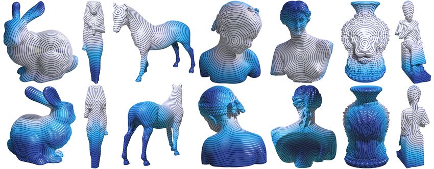
Geodesics in Heat:A New Approach to Computing Distance Based on Heat Flow                                          •      3

Fig. 5. Outline of the heat method. (I) Heat u is allowed to diffuse for a
brief period of time (left). (II) The temperature gradient ∇u (center left) is
normalized and negated to get a unit vector field X (center right) pointing
along geodesics. (III) A function φ whose gradient follows X recovers the
final distance (right).

3.    THE HEAT METHOD
Our method can be described purely in terms of operations on
smooth manifolds; we explore spatial and temporal discretiza-
tion in Sections 3.1 and 3.2, respectively. Let ∆ be the negative-
semidefinite Laplace–Beltrami operator acting on (weakly) differ-                      Fig. 6. Left: Varadhan’s formula. Right: the heat method. Even for very
entiable real-valued functions over a Riemannian manifold (M, g).                      small values of t, simply applying Varadhan’s formula does not provide an
The heat method consists of three basic steps:                                         accurate approximation of geodesic distance (top left); for large values of t
                                                                                       spacing becomes even more uneven (bottom left). Normalizing the gradient
                                                                                       results in a more accurate solution, as indicated by evenly spaced isolines
Algorithm 1 The Heat Method                                                            (top right), and is also valuable when constructing a smoothed distance
   I. Integrate the heat flow u̇ = ∆u for some fixed time t.                           function (bottom right).
  II. Evaluate the vector field X = −∇u/|∇u|.
 III. Solve the Poisson equation ∆φ = ∇ · X.                                           Section 3.2). We can get a better understanding of solutions to
                                                                                       Eq. (3) by considering the elliptic boundary value problem
                                                                                                              (id − t∆)vt = 0 on            M \γ
   The function φ approximates geodesic distance, approaching the                                                                                                    (4)
                                                                                                                       vt = 1 on            γ.
true distance as t goes to zero (Eq. (1)). Note that the solution to step
III is unique only up to an additive constant – final values simply                    which for a point source yields a solution vt equal to ut up to a
need to be shifted such that the smallest distance is zero. Initial                    multiplicative constant. As established by Varadhan in his proof of
conditions u0 = δ(x) (i.e., a Dirac delta) recover the distance to                     Eq. (1), vt also has a close relationship with distance, namely
a single source point x ∈ M as in Figure 1, but in general we can                                                           √
                                                                                                                             t
compute the distance to any piecewise submanifold γ by setting u0                                                   lim −   2
                                                                                                                                 log vt = φ                          (5)
                                                                                                                    t→0
to a generalized Dirac [Villa 2006] over γ (see Figures 3 and 4).
   The heat method can be motivated as follows. Consider an                            away from the cut locus. This relationship ensures the validity of
approximation ut of heat flow for a fixed time t. Unless ut ex-                        steps II and III since the transformation applied to vt preserves the
hibits precisely   the right rate of decay, Varadhan’s transformation                  direction of the gradient.
         √
ut 7→ −4t log ut will yield a poor approximation of the true
geodesic distance φ because it is highly sensitive to errors in mag-                   3.2     Spatial Discretization
nitude (see Figures 2 and 6). The heat method asks for something                       In principle the heat method can be applied to any domain with a
different: it asks only that the gradient ∇ut points in the right direc-               discrete gradient (∇), divergence (∇·) and Laplace operator (∆).
tion, i.e., parallel to ∇φ. Magnitude can safely be ignored since we                   Note that these operators are highly local and hence do not exhibit
know (from the eikonal equation) that the gradient of the true dis-                    significant cancellation error despite large global variation in ut .
tance function has unit length. We therefore compute the normalized
gradient field X =R −∇u/|∇u| and find the closest scalar potential                        3.2.1 Simplicial Meshes. Let u ∈ R|V | specify a piecewise
φ by minimizing M |∇φ − X|2 , or equivalently, by solving the                          linear function on a triangulated surface. A standard discretization
corresponding Euler-Lagrange equations ∆φ = ∇ · X [Schwarz                             of the Laplacian at a vertex i is given by
1995]. The overall procedure is depicted in Figure 5.
                                                                                                    1 X
                                                                                         (Lu)i =            (cot αij + cot βij )(uj − ui ),
3.1    Time Discretization                                                                         2Ai j

We discretize the heat equation from step I of Algorithm 1 in time                        where Ai is one third the area of all trian-
using a single backward Euler step for some fixed time t. In practice,                 gles incident on vertex i, the sum is taken over
this means we simply solve the linear equation                                         all neighboring vertices j, and αij , βij are the
                            (id − t∆)ut = u0                              (3)          angles opposing the corresponding edge [Mac-
                                                                                       Neal 1949]. We can express this operation via
over the entire domain M , where id is the identity (here we still                     a matrix L = A−1 LC , where A ∈ R|V |×|V | is
consider a smooth manifold; spatial discretization is discussed in                     a diagonal matrix containing the vertex areas and LC ∈ R|V |×|V | is
                                                                                 ACM Transactions on Graphics, Vol. 32, No. 3, Article XXX, Publication date: Month 2013.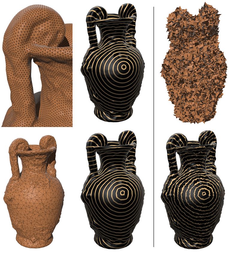
4      •       K. Crane et al.

Fig. 7. Since the heat method is based on well-established discrete opera-
tors like the Laplacian, it is easy to adapt to a variety of geometric domains.
Above: distance on a hippo composed of high-degree nonplanar (and some-
times nonconvex) polygonal faces.
                                                        Hippo mesh courtesy Luxology LLC.

the cotan operator representing the remaining sum. Heat flow can
then be computed by solving the symmetric positive-definite system
                                                                                            Fig. 8. The heat method can be applied directly to point clouds that lack
                             (A − tLC )u = δγ                                               connectivity information. Left: face scan with holes and noise. Right: kitten
                                                                                            surface with connectivity removed. Yellow points are close to the source;
   where δγ is a Kronecker delta over γ (the mass ma-                                       disconnected clusters (in the sense of Liu et al.) receive a constant red value.
trix A need not appear on the right-hand side – a Kro-                                                                                               Kitten mesh courtesy AIM@Shape.

necker delta already gives the integrated value of a
Dirac delta). The gradient in a given triangle can be                                       therefore approximate the magnitude of the gradient as
expressed succinctly as
                                                                                                                                 s
                             1 X                                                                                                     uTf Lf uf
                       ∇u =       ui (N × ei )                                                                        |∇u|f =                    .
                            2Af i                                                                                                       Af

   where Af is the area of the face, N is its unit                                          This quantity is used to normalize the 1-form values associated with
normal, ei is the ith edge vector (oriented counter-                                        half edges in the corresponding face. The integrated divergence is
clockwise), and ui is the value of u at the opposing                                        then given by dT M α where α is the normalized gradient, d is the
vertex. The integrated divergence associated with ver-                                      coboundary operator and M is the mass matrix for 1-forms (see
tex i can be written as                                                                     [Alexa and Wardetzky 2011] for details). These operators are applied
                   1X                                                                       in steps I-III as usual. Figure 7 demonstrates distance computed on
         ∇·X =           cot θ1 (e1 · Xj ) + cot θ2 (e2 · Xj )                              an irregular polygonal mesh.
                   2 j

where the sum is taken over incident triangles j each with a vec-                              3.2.3 Point Clouds. For a discrete point sample P ⊂ Rn of M
tor Xj , e1 and e2 are the two edge vectors of triangle j containing i,                     with no connectivity information, we solve the heat equation (step
and θ1 , θ2 are the opposing angles. If we let b ∈ R|V | be the vector                      I) using the point cloud Laplacian recently introduced by Liu et
of (integrated) divergences of the normalized vector field X, then                          al. [2012], which extends previous work of Belkin et al. [2009a]. In
the final distance function is computed by solving the symmetric                            this formulation, the Laplacian is represented by A−1   V LP C , where
Poisson problem                                                                             AV is a diagonal matrix of Voronoi areas and LP C is symmetric
                                                                                            positive semidefinite (see [Liu et al. 2012], Section 3.4, for details).
                                  LC φ = b.                                                    To compute the vector field X = −∇u/|∇u| (step II), we repre-
Conveniently, this discretization easily generalizes to higher di-                          sent the function u : P → R as a height function over approximate
mensions (e.g., tetrahedral meshes) using well-established discrete                         tangent planes Tp at each point p ∈ P and evaluate the gradient
operators; see for instance [Desbrun et al. 2008].                                          of a weighted least squares (WLS) approximation of u [Nealen
                                                                                            2004]. This approximation provides a discrete gradient operator
   3.2.2 Polygonal Surfaces. For a mesh with (not necessarily                               D ∈ R|P |×|P | . To compute tangent planes, we use a moving least
planar) polygonal faces, we use the polygonal Laplacian defined by                          squares (MLS) approximation for simplicity, although other choices
Alexa and Wardetzky [2011]. The only difference in this setting is                          are possible (see Liu et al.). To find the best-fit scalar potential φ
that the gradient of the heat kernel is expressed as a discrete 1-form                      (step III), we solve the linear, positive-semidefinite Poisson equation
associated with half edges, hence we cannot directly evaluate the                           LP C φ = DT AV X. Figure 8 shows two examples.
magnitude of the gradient |∇u| needed for the normalization step                               Other discretizations are certainly possible (see for instance [Luo
(Algorithm 1, step II). To resolve this issue we assume that ∇u is                          et al. 2009]); we picked one that was simple to implement in any
constant over each face, implying that                                                      dimension. Note that the computational cost of the heat method
                            Z                                                               depends primarily on the intrinsic dimension n of M , whereas
               uTf Lf uf =      |∇u|2 dA = |∇u|2 Af ,                                       methods based on fast marching require a grid of the same dimension
                                 M                                                          m as the ambient space [Memoli and Sapiro 2001] – this distinction
where uf is the vector of heat values in face f , Af is the magnitude                       is especially important in contexts like machine learning where m
of the area vector, and Lf is the local (weak) Laplacian. We can                            may be significantly larger than n.
ACM Transactions on Graphics, Vol. 32, No. 3, Article XXX, Publication date: Month 2013.
Geodesics in Heat:A New Approach to Computing Distance Based on Heat Flow                             •      5

   3.2.4 Choice of Time Step. Accuracy of the heat method relies
in part on the time step t. In the smooth setting, Eq. (5) suggests
that smaller values of t yield better approximations of geodesic
distance. In the discrete setting we instead discover that the limit
solution to Eq. (3) is purely a function of the combinatorial distance,
independent of how we discretize the Laplacian (see Appendix A).
Therefore, on a fixed mesh decreasing the value of t does not nec-
essarily improve accuracy, even in exact arithmetic. (Of course, we
can always improve accuracy by refining the mesh and decreasing
t accordingly.) Moreover, large values of t produce a smoothed
approximation of geodesic distance (Section 3.3). We therefore seek
an optimal time step t∗ that is neither too large nor too small.
   Determining a provably optimal expression for t∗ is difficult
due to the complexity of analysis involving the cut locus [Neel
and Stroock 2004]. We instead use a simple estimate that works
remarkably well in practice, namely t = mh2 where h is the mean
spacing between adjacent nodes and m > 0 is a constant. This
estimate is motivated by the fact that h2 ∆ is invariant with respect
to scale and refinement; experiments on a regular grid (Figure 18)
suggest that m = 1 is the smallest parameter value that recovers the
`2 distance, and indeed this value yields near-optimal accuracy for a
wide variety of irregularly triangulated surfaces, as demonstrated in
Figure 20. In this paper the time step                                                    Fig. 10. Top row: our smoothed approximation of geodesic distance (left)
                                                                                          and biharmonic distance (center) both mitigate sharp “cusps” found in the
                                                                                          exact distance (right), yet isoline spacing of the biharmonic distance can
                                                 t = h2                                   vary dramatically. Bottom row: biharmonic distance (center) tends to exhibit
                                                                                          elliptical level lines near the source, while our smoothed distance (left)
is therefore used uniformly throughout all tests and examples, except                     maintains isotropic circular profiles as seen in the exact distance (right).
where we explicitly seek a smoothed approximation of distance,                            Camel mesh courtesy AIM@Shape.
as in Section 3.3. For highly nonuniform meshes one could set h
to the maximum spacing, providing a more conservative estimate.                              In contrast, one can rapidly construct smoothed approximations
Numerical underflow could theoretically occur for extremely small                         of geodesic distance by simply applying the heat method for large
t, though we do not encounter this issue in practice.                                     values of t (Figure 9). The computational cost remains the same, and
                                                                                          isolines are evenly spaced for any value of t due to normalization
3.3        Smoothed Distance                                                              (step II); the solution is isometrically invariant since it depends
                                                                                          only on intrinsic differential operators. For a time step t = mh2 ,
Geodesic distance fails to be smooth at points in the cut locus, i.e.,                    meaningful values of m are found in the range 1 − 106 – past this
points at which there is no unique shortest path to the source – these                    point the term t∆ dominates, resulting in little visible change.
points appear as sharp cusps in the level lines of the distance function.                    Existing smooth distance functions can also be understood in
Non-smoothness can result in numerical difficulty for applications                        terms of time-discrete heat flow. In particular, the commute-time
which need to take derivatives of the distance function φ (e.g., level                    distance dC and biharmonic distance dB can be expressed in terms
set methods), or may simply be undesirable aesthetically.                                 of the harmonic and biharmonic Green’s functions gC and gB :
   Several distances have been designed with smoothness in mind,
including diffusion distance [Coifman and Lafon 2006], commute-                                       dC (x, y)2 = gC (x, x) − 2gC (x, y) + gC (y, y),
time distance [Fouss et al. 2007], and biharmonic distance [Lipman                                    dB (x, y)2 = gB (x, x) − 2gB (x, y) + gB (y, y).
et al. 2010] (see the last reference for a more detailed discussion).
These distances satisfy a number of important properties (smooth-                         On a manifold of constant sectional curvature the sum g(x, x) +
ness, isometry-invariance, etc.), but are poor approximations of true                     g(y, y) is constant. Locally, then, commute-time and biharmonic
geodesic distance, as indicated by uneven spacing of isolines (see                        distance look like the harmonic and biharmonic Green’s functions
Figure 10, middle). They can also be expensive to evaluate, requir-                       (respectively), which can be expressed via one- and two-step back-
ing either a large number of Laplacian eigenvectors (∼ 150 − 200                          ward Euler approximations of heat flow:
in practice) or the solution to a linear system at each vertex.                                                gC = limt→∞ (id − t∆)† δ,
                                                                                                               gB = limt→∞ (id − 2t∆ + t2 ∆2 )† δ.
                                                                                          (Here † denotes the pseudoinverse.)

                                                                                          3.4       Boundary Conditions
                                                                                          When computing the exact distance, either vanishing Neumann or
                                                                                          Dirichlet conditions suffice since this choice does not affect the
                                                                                          behavior of the smooth limit solution (see [von Renesse 2004],
                                                                                          Corollary 2 and [Norris 1997], Theorem 1.1, respectively). Bound-
Fig. 9. A source on the front of the Stanford Bunny results in nonsmooth
cusps on the opposite side. By running heat flow for progressively longer                 ary conditions do however alter the behavior of our smoothed dis-
durations t, we obtain smoothed approximations of geodesic distance (right).              tance. Although there is no well-defined “correct” behavior for this
Bunny mesh courtesy Stanford Computer Graphics Laboratory.                                smoothed function, we advocate the use of averaged boundary con-
                                                                                    ACM Transactions on Graphics, Vol. 32, No. 3, Article XXX, Publication date: Month 2013.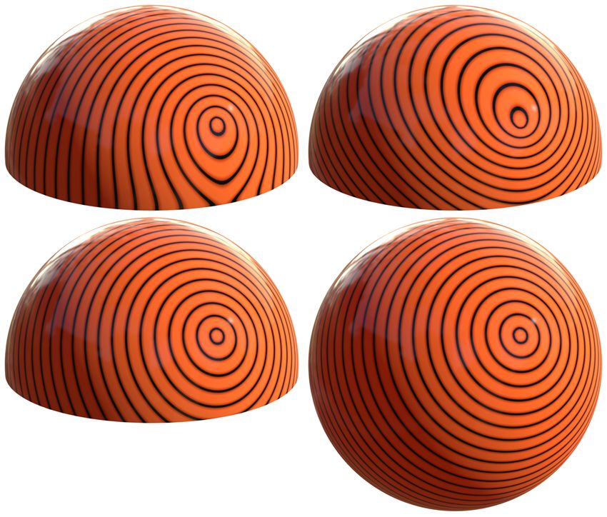
6      •       K. Crane et al.

                                                                                           4.    EVALUATION
                                                                                           4.1    Performance
                                                                                              A key advantage of the heat
                                                                                           method is that the linear systems in
                                                                                           steps (I) and (III) can be prefactored.
                                                                                           Our implementation uses sparse
                                                                                           Cholesky factorization [Chen et al.
                                                                                           2008], which for Poisson-type
                                                                                           problems has guaranteed sub-
                                                                                           quadratic complexity but in practice
                                                                                           scales even better [Botsch et al.
                                                                                           2005]; moreover there is strong evidence to suggest that sparse
                                                                                           systems arising from elliptic PDEs can be solved in very close to
                                                                                           linear time [Schmitz and Ying 2012; Spielman and Teng 2004].
                                                                                           Independent of these issues, the amortized cost for problems with
                                                                                           a large number of right-hand sides is roughly linear, since back
                                                                                           substitution can be applied in essentially linear time. See inset for a
Fig. 11. Effect of Neumann (top-left), Dirichlet (top-right) and averaged                  breakdown of relative costs in our implementation.
(bottom-left) boundary conditions on smoothed distance. Averaged boundary                  In terms of absolute performance, a number of factors affect the
conditions mimic the behavior of the same surface without boundary.                        run time of the heat method including the spatial discretization,
                                                                                           choice of discrete Laplacian, geometric data structures, and so forth.
                                                                                           As a typical example, we compared our simplicial implementation
                                                                                           (Section 3.2.1) to the first-order fast marching method of Kimmel &
                                                                                           Sethian [1998] and the exact algorithm of Mitchell et al. [1987] as
                                                                                           described by Surazhsky et al. [2005]. In particular we used the state-
                                                                                           of-the-art fast marching implementation of Peyré and Cohen [2005]
                                                                                           and the exact implementation of Kirsanov [Surazhsky et al. 2005].
                                                                                           The heat method was implemented in ANSI C in double precision
                                                                                           using a simple vertex-face adjacency list. Performance was mea-
                                                                                           sured using a single core of a 2.4 GHz Intel Core 2 Duo (Table I).
                                                                                           Note that even for a single distance computation the heat method
                                                                                           outperforms fast marching; more importantly, updating distance for
                                                                                           new subsets γ is consistently an order of magnitude faster (or more)
                                                                                           than both fast marching and the exact algorithm.

                                                                                           4.2    Accuracy
                                                                                           We examined errors in the heat method, fast marching [Kimmel and
                                                                                           Sethian 1998], and the polyhedral distance [Mitchell et al. 1987],
                                                                                           relative to mean edge length h on triangulated surfaces. Figures 21
                                                                                           and 22 illustrate convergence on simple geometries where the exact
                                                                                           distance can be easily obtained. Both fast marching and the heat
                                                                                           method appear to exhibit linear convergence; it is interesting to
Fig. 12. For path planning, the behavior of geodesics can be controlled via                note that even the exact polyhedral distance provides only quadratic
boundary conditions and the time step t. Top-left: Neumann conditions en-                  convergence. Keeping this fact in mind, Table I uses the polyhedral
courage boundary adhesion. Top-right: Dirichlet conditions encourage avoid-                distance as a baseline for comparison on more complicated geome-
ance. Bottom-left: small values of t yield standard straight-line geodesics.               tries – M AX is the maximum error as a percentage of mesh diameter
Bottom-right: large values of t yield more natural trajectories.                           and M IN is the mean relative error at each vertex (a convention
                                                                                           introduced in [Surazhsky et al. 2005]). Note that fast marching tends
                                                                                           to achieve a smaller maximum error, whereas the heat method does
ditions obtained by taking the mean of the Neumann solution uN                             better on average. Figure 14 gives a visual comparison of accuracy;
and the Dirichlet solution uD , i.e., u = 21 (uN + uD ). These condi-                      the only notable discrepancy is a slight smoothing at sharp cusps,
tions tend to produce isolines that are not substantially influenced by                    which may explain the slightly larger maximum error exhibited by
the shape of the boundary (Figures 11 and 19). The intuition behind                        the heat method. Figure 15 indicates that this phenomenon does
this behavior again stems from a random walker interpretation: zero                        not interfere with the extraction of the cut locus – here we simply
Dirichlet conditions absorb heat, causing walkers to “fall off” the                        visualize values of |∆φ| above a fixed threshold. Figure 23 plots
edge of the domain. Neumann conditions prevent heat from flowing                           the maximum violation of metric properties – both the heat method
out of the domain, effectively “reflecting” random walkers. Aver-                          and fast marching exhibit small approximation errors that vanish
aged conditions mimic the behavior of a domain without boundary:                           under refinement. Even for smoothed distance (m >> 1) the triangle
the number of walkers leaving equals the number of walkers return-                         inequality is violated only for highly degenerate geodesic triangles,
ing. Figure 12 shows how boundary conditions affect the behavior                           i.e., all three points on a common geodesic. In contrast, smoothed
of geodesics in a path-planning scenario.                                                  distances discussed in Section 2 satisfy metric properties exactly,
ACM Transactions on Graphics, Vol. 32, No. 3, Article XXX, Publication date: Month 2013.
Geodesics in Heat:A New Approach to Computing Distance Based on Heat Flow                                                                  •        7

                                  Fig. 13. Meshes used in Table I. Left to right: B UNNY, I SIS, H ORSE, B IMBA, A PHRODITE, L ION, R AMSES1 .

               Table I. Comparison with fast marching and exact polyhedral distance. Best speed/accuracy in bold; speedup in orange.
       M ODEL           T RIANGLES                                  H EAT M ETHOD                                                         FAST M ARCHING                                       E XACT
                                           P RECOMPUTE         S OLVE      M AX E RROR       M EAN E RROR                T IME           M AX E RROR  M EAN E RROR                              T IME
      B UNNY                  28k              0.21s         0.01s (28x)      3.22%             1.12%                     0.28s             1.06%        1.15%                                  0.95s
          I SIS               93k              0.73s         0.05s (21x)      1.19%             0.55%                     1.06s             0.60%        0.76%                                  5.61s
      H ORSE                  96k              0.74s         0.05s (20x)      1.18%             0.42%                     1.00s             0.74%        0.66%                                  6.42s
      K ITTEN                106k              1.13s         0.06s (22x)      0.78%             0.43%                     1.29s             0.47%        0.55%                                  11.18s
      B IMBA                 149k              1.79s         0.09s (29x)      1.92%             0.73%                     2.62s             0.63%        0.69%                                  13.55s
A PHRODITE                   205k              2.66s         0.12s (47x)      1.20%             0.46%                     5.58s             0.58%        0.59%                                  25.74s
      L ION                  353k              5.25s         0.24s (24x)      1.92%             0.84%                    10.92s             0.68%        0.67%                                  22.33s
   R AMSES                   1.6M              63.4s         1.45s (68x)      0.49%             0.24%                    98.11s             0.29%        0.35%                                 268.87s

                                                                                           but cannot be used to obtain the true geometric distance. Overall,
                                                                                           the heat method exhibits errors of the same order and magnitude as
                                                                                           fast marching (at lower computational cost) and is therefore suitable
                                                                                           in applications where fast marching is presently used.
                                                                                              The accuracy of the heat method depends on the particular choice
                                                                                           of spatial discretization, and might be further improved by con-
                                                                                           sidering an alternative discrete Laplacian (see for instance [Belkin
                                                                                           et al. 2009b; Hildebrandt and Polthier 2011]). In the case of fast
                                                                                           marching, accuracy is determined by the choice of update rule. A
                                                                                           number of highly accurate update rules have been developed for
                                                                                           regular grids (e.g., HJ WENO [Jiang and Peng 1997]), but fewer
                                                                                           options are available on irregular domains such as triangle meshes,
                                                                                           the predominant choice being the first-order update rule of Kimmel
                                                                                           and Sethian [1998]. Finally, the approximate algorithm of Surazhsky
                                                                                           et al. provides an interesting comparison since it tends to produce
                                                                                           results more accurate than fast marching at a similar computational
                                                                                           cost. However, one should be careful to note that accuracy is mea-
                                                                                           sured relative to the polyhedral distance rather than the smooth
                                                                                           geodesic distance of the approximated surface (see [Surazhsky et al.
                                                                                           2005], Table 1). Similar to fast marching, Surazhsky’s method does
                                                                                           not take advantage of precomputation and therefore exhibits a signif-
                                                                                           icantly higher amortized cost than the heat method; it is also limited
Fig. 14. Visual comparison of accuracy. Left: exact geodesic distance.                     to triangle meshes.
Using default parameters, the heat method (middle) and fast marching (right)
both produce results of comparable accuracy, here within less than 1% of
the exact distance – see Table I for a more detailed comparison.                           1 Bunny mesh courtesy Stanford Computer Graphics Laboratory. Isis, Horse, Bibma, Lion, and Ramses meshes courtesy
Kitten mesh courtesy AIM@Shape.                                                            AIM@Shape. Aphrodite mesh courtesy Jotero GbR.

                                                                                     ACM Transactions on Graphics, Vol. 32, No. 3, Article XXX, Publication date: Month 2013.
8        •        K. Crane et al.

Fig. 15. Medial axis of the hiragana letter “a” extracted by thresholding
second derivatives of the distance to the boundary. Left: fast marching. Right:
heat method.

4.3       Robustness
                                                                                           Fig. 17. Smoothed geodesic distance on an extremely poor triangulation
Two factors contribute to the robustness of the heat method, namely                        with significant noise – note that small holes are essentially ignored. Also
(1) the use of an unconditionally stable implicit time-integration                         note good approximation of distance even along thin slivers in the nose.
scheme and (2) formulation in terms of elliptic PDEs. Figure 16
verifies that the heat method continues to work well even on meshes
that are poorly discretized or corrupted by a large amount of noise
                                                                                           5.   CONCLUSION
(here modeled as uniform Gaussian noise applied to the vertex                              The heat method is a simple, general method that can be easily
coordinates). In this case we use a moderately large value of t to                         incorporated into a broad class of algorithms. However, a great deal
investigate the behavior of our smoothed distance; similar behavior                        remains to be explored, including an investigation of alternative
is observed for small t values. Figure 17 illustrates the robustness                       spatial discretizations. Further optimization of the parameter t also
of the method on a surface with many small holes as well as long                           provides an avenue for future work (especially in the case of variable
sliver triangles.                                                                          spacing), though one should note that the existing estimate already
                                                                                           outperforms fast marching in terms of mean error (Table I). Another
                                                                                           obvious question is whether a similar transformation can be applied
                                                                                           to a larger class of Hamilton-Jacobi equations – for instance, a vari-
                                                                                           able speed function might be incorporated by locally rescaling the
                                                                                           metric. Finally, weighted distance computation might be achieved
                                                                                           by simply rescaling the source data.

                                                                                           REFERENCES

                                                                                           Marc Alexa and Max Wardetzky. 2011. Discrete Laplacians on General
                                                                                              Polygonal Meshes. ACM Trans. Graph. 30, 4 (2011), 102:1–102:10.
                                                                                           Mikhail Belkin, Jian Sun, and Yusu Wang. 2009a. Constructing Laplace
                                                                                              operator from point clouds in Rd . In ACM-SIAM Symp. Disc. Alg.
                                                                                           Mikhail Belkin, Jian Sun, and Yusu Wang. 2009b. Discrete Laplace Operator
                                                                                              for Meshed Surfaces. In ACM-SIAM Symp. Disc. Alg. 1031–1040.
                                                                                           D. Bommes and Leif Kobbelt. 2007. Accurate computation of geodesic
                                                                                              distance fields for polygonal curves on triangle meshes. In Proc. Workshop
                                                                                              on Vision, Modeling, and Visualization (VMV). 151–160.
                                                                                           Mario Botsch, David Bommes, and Leif Kobbelt. 2005. Efficient linear sys-
                                                                                              tem solvers for mesh processing. In IMA Conference on the Mathematics
                                                                                              of Surfaces. Springer, 62–83.
                                                                                           Marcel Campen and Leif Kobbelt. 2011. Walking On Broken Mesh: Defect-
                                                                                              Tolerant Geodesic Distances and Parameterizations. Computer Graphics
                                                                                              Forum 30, 2 (2011), 623–632.
                                                                                           P. Chebotarev. 2011. The Walk Distances in Graphs. ArXiv e-prints (2011).
                                                                                           Yanqing Chen, Timothy A. Davis, William W. Hager, and Sivasankaran
                                                                                              Rajamanickam. 2008. Algorithm 887: CHOLMOD, Supernodal Sparse
Fig. 16. Tests of robustness. Left: our smoothed distance (m = 104 )                          Cholesky Factorization and Update/Downdate. ACM Trans. Math. Softw.
appears similar on meshes of different resolution. Right: even for meshes
with severe noise (top) we recover a good approximation of the distance                       35, Article 22 (October 2008), 14 pages. Issue 3.
function on the original surface (bottom, visualized on noise-free mesh).                  Ronald R. Coifman and Stephane Lafon. 2006. Diffusion maps. Appl.
Amphora mesh courtesy AIM@Shape.                                                              Comput. Harmon. Anal. 21 (2006), 5–30.
ACM Transactions on Graphics, Vol. 32, No. 3, Article XXX, Publication date: Month 2013.
Geodesics in Heat:A New Approach to Computing Distance Based on Heat Flow                                         •      9

Mathieu Desbrun, Eva Kanso, and Yiying Tong. 2008. Discrete Differential             Vitaly Surazhsky, Tatiana Surazhsky, Danil Kirsanov, Steven J. Gortler, and
 Forms for Computational Modeling. In Discrete Differential Geometry.                   Hugues Hoppe. 2005. Fast exact and approximate geodesics on meshes.
 Oberwolfach Seminars, Vol. 38. Birkhäuser Verlag, 287–324.                           ACM Trans. Graph. 24 (2005), 553–560. Issue 3.
Francois Fouss, Alain Pirotte, Jean-Michel Renders, and Marco Saerens.               S. R. S. Varadhan. 1967. On the behavior of the fundamental solution of the
  2007. Random-Walk Computation of Similarities between Nodes of a                      heat equation with variable coefficients. Communications on Pure and
  Graph with Application to Collaborative Recommendation. IEEE Trans.                  Applied Mathematics 20, 2 (1967), 431–455.
  on Knowl. and Data Eng. 19, 3 (2007), 355–369.                                     Elena Villa. 2006. Methods of Geometric Measure Theory in Stochastic
Klaus Hildebrandt and Konrad Polthier. 2011. On approximation of the                   Geometry. Ph.D. Dissertation. Università degli Studi di Milano.
  Laplace-Beltrami operator and the Willmore energy of surfaces. Comput.             Max-K. von Renesse. 2004. Heat Kernel Comparison on Alexandrov Spaces
  Graph. Forum 30, 5 (2011), 1513–1520.                                                with Curvature Bounded Below. Potential Analysis 21, 2 (2004).
S. Hysing and S. Turek. 2005. The Eikonal Equation: Numerical Efficiency             Ofir Weber, Yohai S. Devir, Alexander M. Bronstein, Michael M. Bronstein,
  vs. Algorithmic Complexity. In Proc. Algoritmy. 22–31.                                and Ron Kimmel. 2008. Parallel algorithms for approximation of distance
                                                                                        maps on parametric surfaces. ACM Trans. Graph. 27, 4 (2008).
Guangshan Jiang and Danping Peng. 1997. Weighted ENO Schemes for
 Hamilton-Jacobi Equations. SIAM J. Sci. Comput 21 (1997), 2126–2143.
                                                                                     APPENDIX
Ron Kimmel and J.A. Sethian. 1998. Fast Marching Methods on Triangu-
 lated Domains. Proc. Nat. Acad. Sci. 95 (1998), 8341–8435.
Yaron Lipman, Raif M. Rustamov, and Thomas A. Funkhouser. 2010. Bihar-               A.     A VARADHAN FORMULA FOR GRAPHS
  monic Distance. ACM Trans. Graph. 29, Article 27 (July 2010), 11 pages.
                                                                                        L EMMA 1. Let G = (V, E) be the graph induced by nonzeros
  Issue 3.
                                                                                     in any real symmetric matrix A, and consider the linear system
Yang Liu, Balakrishnan Prabhakaran, and Xiaohu Guo. 2012. Point-Based
  Manifold Harmonics. IEEE Trans. Vis. Comp. Graph. 18 (2012).                                                      (I − tA)ut = δ
Chuanjiang Luo, Issam Safa, and Yusu Wang. 2009. Approximating Gradi-                where I is the identity, δ is a Kronecker delta at a source vertex
  ents for Meshes and Point Clouds via Diffusion Metric. Comput. Graph.              u ∈ V , and t > 0 is a real parameter. Then generically
 Forum 28, 5 (2009), 1497–1508.
                                                                                                                                log ut
Richard MacNeal. 1949. The Solution of Partial Differential Equations by                                            φ = lim
  means of Electrical Networks. Ph.D. Dissertation. Caltech.                                                              t→0    log t
F. Memoli and G. Sapiro. 2001. Fast Computation of Weighted Dis-                                      |V |
                                                                                     where φ ∈ N0 is the graph distance (i.e., number of edges) be-
  tance Functions and Geodesics on Implicit Hyper-Surfaces. Journal of
                                                                                     tween each vertex v ∈ V and the source vertex u.
  Comp. Physics 173 (2001), 730–764.
F. Memoli and G. Sapiro. 2005. Distance Functions and Geodesics on                      P ROOF. Let σ be the operator norm of A. Then for t < 1/σ the
  Submanifolds of Rd and Point Clouds. SIAM J. Appl. Math. 65, 4 (2005).             matrix B := I − tA has an inversePand the solution ut is given
                                                                                     by the convergent Neumann series ∞            k k
                                                                                                                             k=0 t A δ. Let v ∈ V be a
J. Mitchell, D. Mount, and C. Papadimitriou. 1987. The discrete geodesic
                                                                                     vertex n edges away from u, and consider the ratio rt := |s|/|s0 |
   problem. SIAM J. of Computing 16, 4 (1987), 647–668.
                                                                                     whereP  s0 := (tn An δ)v is the first nonzero term in the sum and
Andrew Nealen. 2004. An As-Short-As-Possible Intro. to the MLS Method                s=( ∞    k=n+1  tk Ak δ)v is the sum of all remaining terms. Noting
 for Scattered Data Approximation and Interpolation. Technical Report.               that |s| ≤ ∞
                                                                                                P          k    k
                                                                                                                        P∞         k k
                                                                                                  k=n+1 t ||A δ|| ≤       k=n+1 t σ , we get
Robert Neel and Daniel Stroock. 2004. Analysis of the cut locus via the heat                                           ∞
                                                                                                        tn+1 σ n+1 k=0 tk σ k
                                                                                                                    P
  kernel. Surveys in Differential Geometry 9 (2004), 337–349.                                                                           t
                                                                                                  rt ≤                            =c        ,
James Norris. 1997. Heat Kernel Asymptotics and the Distance Function in                                       tn (An δ)v            1 − tσ
  Lipschitz Riemannian Manifolds. Acta Math. 179, 1 (1997), 79–103.                  where the constant c := σ n+1 /(An δ)v does not depend on t. We
G. Peyré and L. D. Cohen. 2005. Prog. in Nonlin. Diff. Eq. and Their                therefore have limt→0 rt = 0, i.e., only the first term s0 is significant
  Applications. Vol. 63. Springer, Chapter Geodesic Computations for Fast            as t goes to zero. But log s0 = n log t + log(An δ)v is dominated
  and Accurate Surface Remeshing and Parameterization, 157–171.                      by the first term as t goes to zero, hence log(ut )v / log t approaches
Anand Rangarajan and Karthik Gurumoorthy. 2011. A Fast Eikonal Equation              the number of edges n.
 Solver using the Schrödinger Wave Equation. Technical Report REP-2011-               Numerical experiments such as those depicted in Figure 18 agree
 512. CISE, University of Florida.                                                   with this analysis. See also [Chebotarev 2011].
Raif Rustamov, Yaron Lipman, and Thomas Funkhouser. 2009. Interior
  Distance Using Barycentric Coordinates. Computer Graphics Forum
 (Symposium on Geometry Processing) 28, 5 (July 2009).
Phillip G. Schmitz and Lexing Ying. 2012. A fast direct solver for elliptic
  problems on general meshes in 2D. J. Comput. Phys. 231, 4 (2012).
G. Schwarz. 1995. Hodge decomposition: a method for solving boundary
  value problems. Springer.
J.A. Sethian. 1996. Level Set Methods and Fast Marching Methods: Evolving
  Interfaces in Computational Geometry, Fluid Mechanics, Computer Vision             Fig. 18. Isolines of log ut / log t computed in exact arithmetic on a regular
  and Materials Science. Cambridge University Press.                                 grid with unit spacing (h = 1). As predicted by Lemma 1, the solution
Daniel A. Spielman and Shang-Hua Teng. 2004. Nearly-linear time al-                  approaches the combinatorial distance as t goes to zero.
 gorithms for graph partitioning, graph sparsification, and solving linear
 systems. In Proc. ACM Symp. Theory Comp. (STOC ’04). ACM, 81–90.
                                                                               ACM Transactions on Graphics, Vol. 32, No. 3, Article XXX, Publication date: Month 2013.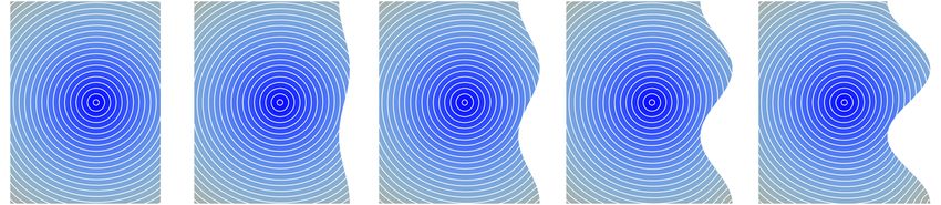
10       •      K. Crane et al.

Fig. 19. Smoothed geodesic distance (m = 1000) using “averaged” bound-
ary conditions. Notice that increasing geodesic curvature along the boundary
does not strongly influence the behavior of the solution.

                                                                                           Fig. 22. Convergence of geodesic distance on the torus at four different test
                                                                                           points. Error is the absolute value of the difference between the numerical
                                                                                           value and the exact (smooth) distance; linear and quadratic convergence are
                                                                                           plotted as dashed lines for reference. Right: test points visualized on the
                                                                                           torus; dark blue lines are geodesic circles computed via Clairaut’s relation.

Fig. 20. Mean percent error as a function of m, where t = mh2 . Each
curve corresponds to a data set from Table I. Notice that in most examples
m = 1 (dashed line) is close to the optimal parameter value (blue dots) and
yields mean error below 1%.

                                                                                           2.0                                               1.5

                                                                                           1.5

                                                                                                                                             1.0

                                                                                           1.0

                                                                                                       0.10   0.15   0.20   0.30    0.50           0.045   0.05    0.055   0.06   0.065 0.07

                                                                                                 5.0

                                                                                                 3.0

                                                                                                 2.0
                                                                                                 1.5

Fig. 21. L∞ convergence of distance functions on the unit sphere with                            1.0
respect to mean edge length. As a baseline for comparison, we use the exact
distance function φ(x, y) = cos−1 (x · y). Linear and quadratic convergence
are plotted as dashed lines for reference; note that even the exact polyhedral
distance converges only quadratically.                                                                           0.015      0.020          0.030           0.050           0.070

                                                                                           Fig. 23. Fast marching and the heat method both exhibit small violations
ACKNOWLEDGMENTS                                                                            of metric properties such as symmetry (top left) and the triangle inequality
This work was funded by a Google PhD Fellowship and a grant                                (top right) that vanish under refinement – we plot the worst violation among
from the Fraunhofer Gesellschaft. Thanks to Michael Herrmann                               all pairs or triples of vertices (respectively) as a percent of mesh diameter.
                                                                                           Dashed lines plot linear convergence. Bottom right: the triangle inequality is
for inspiring discussions, and Ulrich Pinkall for discussions about                        violated only for vertices along a geodesic between two distinguished points
Lemma 1. Meshes are provided courtesy of the Stanford Computer                             (in red), since the corresponding geodesic triangles are nearly degenerate.
Graphics Laboratory, the AIM@Shape Repository, Luxology LLC,                               Bottom left: percent of red vertices as a function of h – each curve represents
and Jotero GbR (http://www.evolution-of-genius.de/).                                       a different value of m sampled from the range [1, 100].
                                                                                           Bunny mesh courtesy Stanford Computer Graphics Laboratory.

Received September 2012; accepted March 2013

ACM Transactions on Graphics, Vol. 32, No. 3, Article XXX, Publication date: Month 2013.
You can also read