Blind Super Resolution of Real-Life Video Sequences - Krest ...
←
→
Page content transcription
If your browser does not render page correctly, please read the page content below
1544                                                                               IEEE TRANSACTIONS ON IMAGE PROCESSING, VOL. 25, NO. 4, APRIL 2016

                        Blind Super Resolution of Real-Life
                                 Video Sequences
Esmaeil Faramarzi, Member, IEEE, Dinesh Rajan, Senior Member, IEEE, Felix C. A. Fernandes, Member, IEEE,
                              and Marc P. Christensen, Senior Member, IEEE

   Abstract— Super resolution (SR) for real-life video sequences
is a challenging problem due to complex nature of the motion
fields. In this paper, a novel blind SR method is proposed to
improve the spatial resolution of video sequences, while the
overall point spread function of the imaging system, motion fields,
and noise statistics are unknown. To estimate the blur(s), first, a
nonuniform interpolation SR method is utilized to upsample the
frames, and then, the blur(s) is(are) estimated through a multi-
scale process. The blur estimation process is initially performed                 Fig. 1.   A sliding window of size M + N + 1 is defined around each
on a few emphasized edges and gradually on more edges as                          LR frame gk . The corresponding HR frame fk is reconstructed using the
the iterations continue. Also for faster convergence, the blur is                 SR operation by fusing the LR frames inside the window. Frames near the
                                                                                  two sides of the video sequence may have shorter lengths.
estimated in the filter domain rather than the pixel domain. The
high-resolution frames are estimated using a cost function that
has the fidelity and regularization terms of type Huber–Markov                    frames when the cut-off frequency of the detector is lower than
random field to preserve edges and fine details. The fidelity term                that of the lens. Temporal aliasing arises in video sequences
is adaptively weighted at each iteration using a masking operation
to suppress artifacts due to inaccurate motions. Very promising                   when the frame rate of the camera is not high enough to
results are obtained for real-life videos containing detailed struc-              capture high frequencies caused by fast moving objects. The
tures, complex motions, fast-moving objects, deformable regions,                  blur in the captured images and videos is the overall effect
or severe brightness changes. The proposed method outperforms                     of different factors such as defocus, motion blur, optical blur,
the state of the art in all performed experiments through both                    and detector’s blur resulting from light integration within the
subjective and objective evaluations. The results are available
online at http://lyle.smu.edu/~rajand/Video_SR/.                                  active area of each detector in the array. The references [3]–[5]
   Index Terms— Video super resolution, blur deconvolution,
                                                                                  provide overviews of different SR approaches.
blind estimation, Huber Markov random field (HMRF).                                  One way to increase the resolution of a video is by over-
                                                                                  laying a sliding window upon each frame and combining all
                      I. I NTRODUCTION                                            frames falling inside the window to build the corresponding
                                                                                  HR frame (Fig. 1) [6]. Then the window slides to the location
M       ULTI-IMAGE super resolution (SR) is the process of
        estimating a high resolution (HR) image by fusing a
series of low-resolution (LR) images degraded by various
                                                                                  of the other frames and the process repeats. For this system
                                                                                  to work, usually a local registration method (such as optical
artifacts such as aliasing, blurring, and noise. Video super                      flow, block-based, pel-recursive, or Bayesian [7]) is required
resolution, by contrast, is the process of estimating a HR                        to accurately estimate the displacement vector of each pixel
video from one or multiple LR videos in order to increase                         or block within the frames. However, local registration may
the spatial and/or temporal resolution(s). The spatial resolution                 not be reliable in some cases, especially when there are com-
of an imaging system depends on the spatial density of the                        plex dynamic changes (e.g. complex 3D motions), nonrigid
detector (sensor) array and the point spread function (PSF) of                    deformations (e.g. flowing water, flickering fire), or changes
the induced detector blur. The temporal resolution, on the other                  in illumination [8].
hand, is influenced by the frame rate and exposure time of the                       Another class of single-video SR techniques is the one
camera [1], [2]. Spatial aliasing appears in images or video                      known as learning-based, patch-based or example-based video
                                                                                  SR [9], [10]. The basic idea is that small space-time patches
  Manuscript received October 7, 2013; revised June 11, 2014 and                  within a video are repeated many times inside the same video
March 30, 2015; accepted January 14, 2016. Date of publication January 28,        or other videos, at multiple spatio-temporal scales. Therefore,
2016; date of current version February 23, 2016. The associate editor
coordinating the review of this manuscript and approving it for publication was   by replacing LR patches in the input video with equivalent
Prof. Sergio Goma.                                                                HR patches from internal/external sources, the resolution can
  E. Faramarzi and F. C. A. Fernandes are with Samsung Research                   be improved. The major advantage of patch-based image/video
America, Richardson, TX 75082 USA (e-mail: e.faramarzi@samsung.com;
felix.f@samsung.com).                                                             SR methods is that motion estimation and object segmentation
  D. Rajan and M. P. Christensen are with Southern Methodist University,          are not required. However, techniques of this group often have
Dallas, TX 75205 USA (e-mail: rajand@lyle.smu.edu; mpc@lyle.smu.edu).             high computational complexity and most of them need offline
  Color versions of one or more of the figures in this paper are available
online at http://ieeexplore.ieee.org.                                             database training. Furthermore, it is necessary that LR patches
  Digital Object Identifier 10.1109/TIP.2016.2523344                              are generated from HR patches by a known PSF.
                       1057-7149 © 2016 IEEE. Personal use is permitted, but republication/redistribution requires IEEE permission.
                            See http://www.ieee.org/publications_standards/publications/rights/index.html for more information.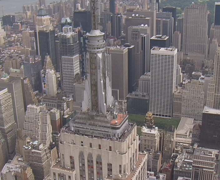
FARAMARZI et al.: BLIND SR OF REAL-LIFE VIDEO SEQUENCES                                                                           1545

   Most works on the image and video SR are non-blind,              to suppress noise while preserving the edges. Unlike in [2],
i.e. they do not consider blur identification during the SR         we discard the output of frame debluring process after the
reconstruction. These methods assume that the PSFs are either       blur estimation is accomplished and perform a non-blind SR
known a priori or negligible, both of which are simplistic          reconstruction to obtain the final estimates of the video frames.
assumptions for realistic applications. For images, there has       To improve the performance of this final frame estimation, the
been a significant amount of publications on blind deconvolu-       fidelity term is weighted adaptively at each iteration pixel by
tion, e.g. [11]–[18], and a few on blind SR, e.g. [2], [19].        pixel. We prove the performance of our proposed method with
However, to the best of our knowledge, there are only               different experiments and comparisons with the state of the art
two independent works on blind SR for videos, which are             methods.
discussed next.                                                        We assume that noise is additive white Gaussian with simi-
   In [20] a method is proposed which uses a total                  lar statistics for all frames and color channels. The blurs in the
variation (TV) prior for frames and a combination of quadratic      input LR video are space-invariant (SI) (identical for all pixels
and TV priors for blurs. The motion is estimated globally           within the frames), spatial (no temporal extension), equal for
either through a phase correlation method or by using an            all color channels (by ignoring the chromatic aberration of the
8-parameter perspective (homography) model. Pixels that are         lens), and either identical or with gradual variations over time.
detected to have inaccurate motion parameters are filtered          However, no prior knowledge about the type and size of the
out from the reconstruction by applying a masking operation.        PSF is required.
A limitation of the work in [20] is that since motion is               In summary, the major differences of this work com-
estimated globally, all regions having local motions need to        pared to our previous one [2] are as follows: 1) processing
be masked out. Therefore, the reconstructed video would be          videos with arbitrary local motions rather than images with
of low quality for all locally-moving objects in the scene which    global and translational motion differences, 2) discussions
could be the most prominent regions to reconstruct. Moreover,       on YCbCr/RGB color spaces and sequential/central motion
results are only presented for PSFs with small spatial support.     estimations, 3) adding a final non-blind frame reconstruction
   In [21] and [22] a Bayesian approach is proposed for             after blur estimation, 4) removing structures finer than the blur
simultaneously estimating the HR frames, motion, blur and           support during motion estimation, 5) using a fidelity term of
noise parameter. The regularization terms for all unknowns          type HMRF rather than quadratic for frame reconstruction to
are of type l1 norm. An estimated noise parameter is used           improve the performance, and 6) using a masking operation
to update the weight of the fidelity term at each iteration of      during frame reconstruction to suppress artifacts.
the optimization procedure. The noise level is updated at each         The usual way to model motion blur in video sequences
iteration, but assumed to be identical for all pixels. The blur     is to define it as a 2D spatial PSF. Using this model, the
kernel is assumed to be separable (h = h x ∗ h y ) and results      PSF would be space-variant (SV) when the scene contains
are only provided with Gaussian blurs. Promising results are        objects that move fast during the exposure time of the camera.
shown for 4× upscaling of real-life videos.                         To reconstruct in such a case, segmentation techniques are
   In [2] we proposed a method for blind deconvolution and          required to separate these objects from the rest of the scene,
super resolution of still images. Similar to most literature on     estimate their motions, deblur them, and then place them back
SR, we assumed the motion fields between the input images to        to the scene in a way that the reconstructed frames seem
be global and translational. In this paper, we extend [2] to the    consistent and artifact-free. This process may be difficult or
case of video sequences with complex motion fields. Errors in       even impossible when the motion blur is so severe that the
the estimated motions make the frame and blur reconstructions       shape of the objects is distorted. However, motion blur has
more challenging, so a careful estimation process is required       a temporal nature [23], [24], so by separating this blur from
to achieve accurate results.                                        other spatial blurring sources and modeling it as a rectangular
   For blur estimation, the input video is first upsampled          temporal PSF with a length equivalent to the exposure time,
(in case of SR) using a nonuniform interpolation (NUI) SR           the overall 3D spatio-temporal PSF would be SI (if spatial
method, then an iterative procedure is applied using the            blurs are all SI). In this paper, we assume that either the motion
following considerations: 1) during the initial iterations, the     blur is global, or the camera’s exposure time is high enough
blur is estimated exclusively using a few emphasized edges          so that no local motion blur appears in the captured videos.
while weak structures are smoothed out, 2) the number of               This paper is organized as follows: Section II discusses the
contributing edges gradually increases as iterations proceed,       SR observation (forward) model, different color spaces for SR
3) structures finer than the blur support are omitted from          processing, and two general approaches for motion estimation.
estimation, 4) the estimation is done in the filter domain rather   The blur estimation procedure is introduced in Section III.
than pixel domain, and finally 5) the estimation is performed       A non-blind SR process to estimate the final HR frames is
at multiple scales to avoid getting trapped in local minima.        discussed in Section IV. Experimental results are presented in
   The cost function used for frame debluring during the blur       Section V, and finally Section VI concludes the paper.
estimation process has fidelity and regularization terms both
of type Huber-Markov Random Field (HMRF). A fidelity term                           II. M ODEL D EFINITION
of this type diminishes outliers caused by inaccurate motion        A. Observation Model
estimation and preserve edges. By contrast, a HMRF prior              As shown in Fig. 1, a sliding window (temporal) of length
exploits the piecewise smoothness nature of the HR frames           M + N + 1 (with M frames backward and N frames forward)
1546                                                                  IEEE TRANSACTIONS ON IMAGE PROCESSING, VOL. 25, NO. 4, APRIL 2016

                                                   g      g
is overlaid around each LR frame gk of size Nx × N y × C,
and all LR frames inside the window are combined through
the SR process to generate the HR reference frame f k of size
   f       f
Nx × N y × C. Here, Nx and N y are frame dimensions in
two spatial directions and C is the number of color channels.
The linear forward imaging model that illustrates the process
of generating a LR frame gi inside the window from the HR                  Fig. 2.       Central motion (blue) versus sequential motion (red).
frame f k is given by:

 gi x ↓ , y↓ ; c = m k,i ( f k (x, y; c)) ∗ h(x, y) ↓L                  In our implementation, video sequences can be processed
                                                                   in either RGB or YUV formats. In the former case, SR is
                  + n k,i x ↓ , y↓ ; c , c = 1, . . . , C,
                                                                     used to increase the resolution of all R, G, and B channels.
                  k = 1, . . . , P, i = k − M, . . . , k + N   (1)
                                                                     However in the latter one, only the Y channel is processed
where P is the total number of frames, (x ↓ , y↓ ) and (x, y)        by SR for faster computation while the Cb and Cr channels
indicate the pixel coordinates in LR and HR image planes             are simply upscaled to the resolution of the super-resolved
respectively, L is the downsampling factor or SR upscaling           Y channel using a single-frame upsampling method such as
                  f         g         f        g
ratio (so that Nx = L Nx and N y = L N y ), and ∗ is the             bilinear or bicubic interpolation. The obtained results related
two-dimensional convolution operator. According to this              to these two cases are comparable using a subjective quality
model, the HR frame f k is warped with the warping func-             assessment.
tion m k,i , blurred by the overall system PSF h, downsampled
by factor L, and finally corrupted by the additive noise n k,i .     C. Motion Estimation
   It is more convenient to express this linear process in the          Accurate motion estimation (registration) with subpixel pre-
vector-matrix notion:                                                cision is crucial for video SR to achieve a good performance.
                      gi = DHMk,i fk + ni                      (2)   Two different approaches can be considered for registration in
                                                                     video SR: central and sequential (Fig. 2). In the former, motion
In (2) fk is the kth HR frame in lexicographical notation            is directly computed between each reference frame and all LR
                              f   f
indicating a vector of size Nx N y C × 1, matrices Mk,i and H        frames inside its sliding window (Fig. 1). By contrast, in the
are the motion (warping) and convolution operators of size           latter, each frame is registered against its previous frame; then
   f  f        f  f
Nx N y C × Nx N y C, D is the downsampling matrix of size            to use with SR, sequential motion fields must be converted
  g    g      f   f                                                                                                                to
Nx N y C × Nx N y C, and gi and ni are vectors of the i th LR        central fields for registration as follows: if Si = Sxi , S yi is
                                              g g
frame and noise respectively, both of size Nx N y C × 1. The         the sequential motion field           frame (w.r.t. the (i −1)th
                                                                                              for the i th
matrix Mk,i registers (or motion compensates) the reference          frame), then Mk,i = Mxk,i , M yk,i , the central motion field
frame fk to match the frame fi . As a result, Mkk is an              for the i th frame when the central frame is the kth frame is
identity (unit) matrix since no motion compensation is required      obtained as:
between a HR frame and its coincident LR frame. For a blur
                                                                                         k
deconvolution (BD) problem (i.e. L = 1), D is the identity            Mk,i = −                 Sn = −Si+1 +Mk,i+1 , k − M ≤ i < k
matrix and so the input and output videos are of the same                            n=i+1
size. Hence BD can be considered as a special case of SR.             Mk,k =         I
The objective in SR and BD is to estimate the HR frames fk
                                                                                         j
and the blur H given the LR frames gi while the motion Mk,i           Mk, j =                  Sn =      S j +Mk, j −1 , k < j ≤ k + N           (3)
and the noise ni are unknown as well.                                                n=k+1

                                                                     where I is the identity matrix.
B. Color Space                                                          With the sequential approach in SR, each frame needs to be
   The human visual system (HVS) is less sensitive to chromi-        registered only against the previous frame, whereas with the
nance (color) than to luminance (light intensity). In the RGB        central approach each frame is registered against all neighbor-
(red, green, blue) color space, the three color components have      ing frames within its reconstruction window. Therefore, the
equal importance and so all are usually stored or processed          computational complexity and the storage size of the motion
at the same resolution. But a more efficient way to take the         fields in the central approach is higher than that of using the
HVS perception into account is by separating the luminance           sequential approach.
from the color information and representing luma with higher            The lower storage size of the motion fields in the sequential
resolution than chroma [25]. A popular way to achieve this           approach is important in applications where the ground-truth
separation is to use the YCbCr color space where Y is                video is available (e.g. when the video to be transmitted is
the luma component (computed as a weighted average of                downsampled intentionally to cope with the bandwidth limi-
R, G, and B) and Cb and Cr are the blue-difference and               tations of the communication channel). In this situation, the
red-difference chroma components. The YUV video format               sequential motion fields estimated from the original video can
is commonly used by video processing algorithms to describe          be used by a SR processing unit at the receiver side to improve
video sequences encoded using YCbCr.                                 the SR performance and also reduce the computational cost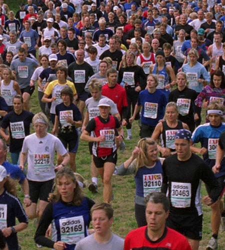
FARAMARZI et al.: BLIND SR OF REAL-LIFE VIDEO SEQUENCES                                                                        1547

(specially in real-time applications). To transmit the motion    where zk = Hfk is the upsampled but still blurry frame.
fields as metadata, they can be either embedded into the         Equation (4) suggests that we can first construct the upsampled
bitstream of the encoded downsampled video (e.g. via the SEI1    frames zk using an appropriate fusion method and then apply
message of AVC2 or HEVC3 video compression standards) or         a deblurring method to zk to estimate fk and h.
sent out separately over the channel along with the video.          If noise characteristics are also the same for all
   Contrary to the sequential approach that should be com-       frames, an appropriate way to estimate zk is using the
puted between successive frames of the same resolution           NUI method [3]–[5]. In NUI, the pixels of all LR frames
(e.g. between bicubically upsampled successive LR frames),       are projected on to the HR image grid according to their
with the central approach a reference HR frame fk can be         motion fields, and then the intensities of the true locations on
directly registered against its LR neighboring frame gi , as     the grid are computed via interpolation [2]. Our experiments
performed in [21] and [22]. This method may result in a more     show that using NUI for upsampling the frames leads to better
accurate estimation for the central approach, although at the    estimates of f and h (Sections III-B and III-C) compared to
cost of more computational complexity for each registration.     when zk is estimated iteratively from the LR frames g using a
   With both sequential and central approach, the motion         MAP (Maximum A Posteriori) or ML (Maximum Likelihood)
fields can be reestimated after several iterations of the blur   method such as [29] and [30].
estimation procedure (Section III) to refine the accuracy of
motion estimates.                                                B. Frame Deblurring
   In our work, we use the sequential approach to estimate         After upsampling the frames, we use the following cost
the motion fields between the successive frames by the use of    function, J , to estimate the HR frames fk having an estimate
dense optical flow method described in [26].                     of the blur h (or H):
                     III. B LUR E STIMATION
                                                                                                          4

                                                                        J (fk ) = ρ (Hfk − zk )1 + λn      ρ ∇ j fk        (5)
   In a multi-channel BD problem, the blurs could be estimated                                                             1
                                                                                                          j =1
accurately along with the HR images [27]. However in a blind
SR problem with a possibly different blur for each frame,        where ·1 denotes the l1 norm  (defined for a sample vector x
some ambiguity in the blur estimation is inevitable due to       with elements x i as x = i |x i | ), λn is the regularization
the downsampling operation [19]. By contrast, in a blind         coefficient, ρ(·) is the vector Huber function, ρ(·)1 is called
SR problem in which all blurs are supposed to be identical       the Huber norm, and ∇ j (i = 1, . . . , 4) are the gradient
or have gradual changes over time, such an ambiguity can be      operators in 0°, 45°, 90° and 135° spatial directions [2]. The
avoided [2]. Moreover, as discussed in Section III-A, the        first term in (5) is called the fidelity term which is the Huber-
assumption of identical (or gradually changing) blurs makes      norm of error between the observed and simulated LR frames.
it possible to separate the registration and upsampling pro-     While in most works the l2 -norm is used for the fidelity
cedures from the deblurring process which significantly          term, we use the robust Huber norm to better suppress the
decreases the blur estimation complexity.                        outliers resulting from inaccurate registration. The next two
   In Section III-A, the NUI method to reconstruct the upsam-    terms in (5) are the regularization terms which apply spatio-
pled frame is explained. This upsampled yet-blurry frame         temporal smoothness to the HR video frames while preserving
is used to estimate the PSF(s) and the deblurred frames          the edges.
through an iterative alternative minimization (AM) process.         Each element of the vector function ρ(·) is the Huber
The blur and frame estimation procedures are discussed in        function defined as:
Sections III-B and III-C, respectively. The estimated frames                            x2          if |x| ≤ T
are used only for the deblurring process and so omitted                       ρ(x) =                                           (6)
                                                                                        2T |x| − T if |x| > T,
                                                                                                  2
thereafter. Finally, the overall AM optimization process is
described in Section III-D.                                      The Huber function ρ(x) is a convex function that has a
                                                                 quadratic form for values less than or equal to a threshold T
A. Frame Upsampling                                              and a linear growth for values greater than T . The Gibbs PDF
  In [2] we discuss the situations in which the warping and      of the Huber function is heavier in the tails than a Gaussian.
blurring operations in (2) are commutable. Although for videos   Consequently, edges in the frames are less penalized with this
with arbitrary local motions this commutability does not hold    prior than with a Gaussian (quadratic) prior.
exactly for all pixels, however we assume here that this is         To minimize the cost function in (5), we use the conjugate
approximately satisfied. The ultimate appropriateness of the     gradient (CG) iterative method [30] because of its simplicity
approximation is validated by the eventual performance of        and efficiency. Compared to some other iterative methods such
the algorithm that is derived based on this model. With this     as Gauss-Seidel (GS) or SOR that need explicit derivation of
assumption, (2) can be rewritten as:                             matrix A when solving a linear equation Ax = b, CG can
                                                                 decompose the matrix A to concatenation of filtering and
            gi = DMk,i Hfk + ni = DMk,i zk + ni            (4)   weighting operations. However, CG can only be used with
 1 Supplemental enhancement information.                         linear equation sets, whereas the cost function in (5) is non-
 2 Advanced Video Coding.                                        quadratic and so its derivative is nonlinear. To overcome this
 3 High Efficiency Video Coding.                                 limitation, we use lagged diffusivity fixed-point (FP) iterative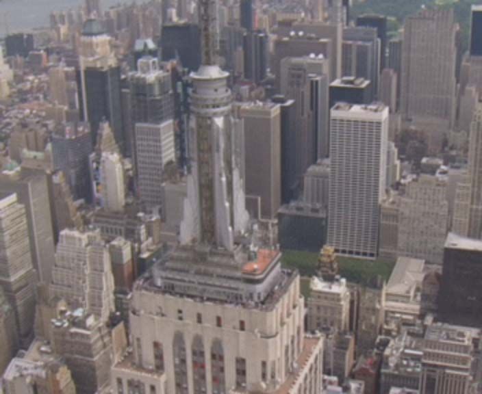
1548                                                                    IEEE TRANSACTIONS ON IMAGE PROCESSING, VOL. 25, NO. 4, APRIL 2016

method [31] to lag the diffusive term by one iteration [15].           Algorithm 1 Blur Estimation Procedure
Using this method for a sample vector x, at the nth iteration
the non-quadratic Huber-norm ρ(xn )1 is replaced by the
following quadratic form:
            n
           ρ(x ) = (xn )T Vn (xn ) = xn 2 n ,         (7)
                   1                        V

where Vn is the following diagonal matrix:

                              1              ˙
                                        xn−1 ≤T
             Vn = diag                                           (8)
                              T /̇x n−1 xn−1 >T
                                             ˙
In (8) the dots above the division and comparison operators
indicate element-wise operations. Applying the FP method
to (5) and setting the derivative of the cost function with
respect to fk to zero results in the following linear equation
set:

                           4
         Hn T Vn Hn + λn          ∇ Tj Wnj ∇ j = Hn T Vn zk ,    (9)
                           j =1

where:
                 Vn = diag ρ(Hfkn−1 − zk ) ,

                Wnj = diag ρ(∇ j fkn−1 )                        (10)

We discuss how to update the regularization parameter λn at
each iteration in Section III-D.

C. Blur Estimation
    Within an image or video frame, non-edge regions and weak
structures are not appropriate for blur estimation. Hence, more
accurate results would be obtained if the estimation is not
performed in such regions. For this reason, in [11] and [33]
the user should first manually select a region with rich edge
structure, whereas in [2], [13], [14], and [34] the most salient       Algorithm 2 Final Frame Estimation Procedure
edges are automatically chosen. Moreover, sharpening salient
edges would also improve the accuracy of blur estimation. The
authors of [34] leveraged these two strategies by preprocessing
blurred images with the shock filtering method proposed
in [35]. Shock filtering is an edge preserving smoothing
operation by which soft edges gradually approach step edges
within a few iterations while non-edge regions are smoothed.
Since shock filtering is sensitive to noise, sometimes a pre-
filtering operation is applied to first suppress noise. For
example, in [13] bilateral filtering (proposed by [36]) is used
and in [14] and [34] a lowpass Gaussian filtering is utilized
before shock filtering. A similar concept for the blur estimation
is exploited in [37] in which the image is first sharpened by
redistributing the pixels along the edge profiles in such a way
that antialiased step edges are produced. Having the sharpened
image and the blurry input image, the blur is then estimated
using a maximum a posteriori (MAP) framework.
    In our work, we employ the edge-preserving smoothing               through l0 gradient minimization using the following cost
method of [40] in which the number of surviving edges                  function:
                                                                               n  n             2
after smoothing is globally controlled by the regularization                J f  k = f  k − fkn 2 + β n ∇x f  0 + ∇ y f  0 , (11)
coefficient. This feature is helpful when one desires to limit
the number of salient edges at each iteration. This smoothing          where f  nk is the output of the edge-preserving smoothing
method aims to keep an intended number of non-zero gradients           algorithm and the l0 norm is defined as x0 = # (i |x i = 0).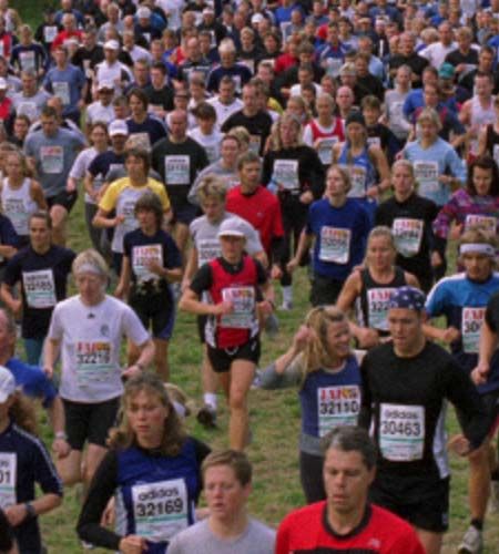
FARAMARZI et al.: BLIND SR OF REAL-LIFE VIDEO SEQUENCES                                                                                                1549

Fig. 3. Reconstruction result for the City video sequence (please zoom into the figure on screen; see the videos at http://lyle.smu.edu/~rajand/Video_SR/).
(a) Ground-truth frame; (b) LR frame by applying a Gaussian PSF with σ = 1.2 having size of 15 × 15, downsampling ratio of 2, and Gaussian noise with
SNR of 30d B, then upsampled to the original resolution using Bicubic; (c) Original blur; (d) Smoothed frame; (e) Negative of gradient magnitude of (d);
(f) Salient edges not narrower than the kernel support; (g) Result of 3D-ISKR [38] deblurred by [39] with PSNR of 28.9d B (after border removal); (h) Result
of our proposed method with PSNR of 32.4 dB; (i) Estimated blur with NMSE of 0.1.

                                                                                                                    2             −1
Unlike shock filtering, this smoothing method does not need                                         b = ∇x + ∇ y =                                    (14)
pre-filtering of noise.                                                                                            −1             0
   Though sufficient edge pixels are required for accurate blur                  In (13) and (14), a is the all-ones filter of size 11 × 11
estimation, it is shown in [14] that structures with scales                    and b is the sum-of-gradients filter. According to (12)-(14),
smaller than the PSF support could harm blur estimation.                       to compute Rkn , the sum of gradient components of f  nk is
Inspired by that work, we define Rkn in (12) to measure the                    computed first, then at each pixel it is summed up with
usefulness of each pixel for blur estimation:                                  the values of all neighboring pixels, and finally its absolute
                                    n
                        Rkn = ABf  k  ,                 (12)                value is obtained. For pixels on narrow structures, the sum of
                                                                               gradient values cancels out each other. Therefore, Rkn usually
where A and B are the convolution operators for the spatial                    has a small value at the location of narrow edges and smooth
filters a and b, respectively, as defined below:                               regions. Then f  nk is refined by only retaining strong and
                      ⎡               ⎤                                        non-spike edges:
                         1 ··· 1
                      ⎢               ⎥
                  a = ⎣ ... . . . ... ⎦               (13)                                 n     ∇f  nk if ∇f  nk  >T
                                                                                                                         ˙ 1n and Rkn >T
                                                                                                                                      ˙ 2n
                                                                                       ∇f k =                                              (15)
                            1    ···    1                                                          0       otherwise,
1550                                                                             IEEE TRANSACTIONS ON IMAGE PROCESSING, VOL. 25, NO. 4, APRIL 2016

Fig. 4. Experimental results for the Mobile video sequence (please zoom into the figure on screen; see the videos at http://lyle.smu.edu/~rajand/Video_SR/).
(a) Ground-truth video frame. (b) One LR frame generated by applying a 5 × 5 out-of-focus blur having size of 15 × 15, spatial downsampling of 2, and
Gaussian noise with SNR of 30d B, then upsampled to the original resolution using Bicubic; (c) Original blur; (d) Reconstruction result of 3D-ISKR [38]
deblurred by [39] with PSNR of 20.8d B; (e) Reconstruction result of our proposed method with PSNR of 22.7d B; (f) The estimated PSF with NMSE
of 0.15.

where T1n and T2n are threshold parameters which decrease at                   where ∇i (i = 1, 2) is ∇x or ∇ y , F (·) and F −1 (·) are FFT
each iteration.                                                                and inverse-FFT operations, and (·) is the complex conjugate
  In our work, the blur is estimated from the gradients of                     operator. We then apply the following constraints to the
zk and f  k instead of their pixel values since estimation in                estimated PSF: its negative values are set to zero, then the PSF
the filter domain converges faster than the pixel domain. The                  is normalized to the range [0, 1], and centered in its support
reason for faster convergence is that in a linear equation set                 window.
Ah = b (derived from a quadratic cost function defined for h),
matrix A would be better conditioned when the gradients of
images are used [13].                                                          D. Overall Optimization for Blur Estimation
  To avoid ringing artifact, we apply the MATLAB function                         The overall optimization procedure for estimating the PSF
edgetaper() to ∇f  nk . Then we estimate each blur hk using the              is shown in Algorithm 1. The HR frames and the PSF
cost function J (h) below:                                                     are sequentially updated within the AM iterations. We use
                                                                               a multi-scale approach to avoid trapping in local minima.

                    P1

          J (h) =      ∇zk − ∇F k h2 + γ n ∇h2 ,                 (16)    The regularization coefficients λn in (9) and γ n in (17)
                                       2           2
                    k=1
                                                                               decrease at each AM (alternating minimization) iteration
                                                                               up to some minimum values λmin and γmin , respectively
where P1 ≤ M + N and F k is the convolution matrix of f  k .               (see [2] for a discussion). The variation of these coefficients is
Since J (h) in (16) is quadratic, it can be easily minimized by                given by:
pixel-wise division in the frequency domain [41] as:
                                                                                                     λn = max r λn−1 , λmin ,
h nk (x, y)
                 2                                                                                 γ n = max r γ n−1 , γmin                         (18)
        −1

              P1

  =F                   F (∇i )×F            ˙ F (∇i )×F
                              ˙ ( f  nk ) ×        ˙ (z k )
              k=1 i=1                                                          where r is a scalar less than 1. Also the values of β n in (11)
                                                                           and T1n and T2n in (15) fall at each AM iteration which
                                   n 2̇
               /̇ F (∇i )×∇(
                          ˙   f  k ) + γ n |F (∇i )|2̇              (17)    increases the number of contributing pixels to blur estimation
                                                                               as the optimization proceeds.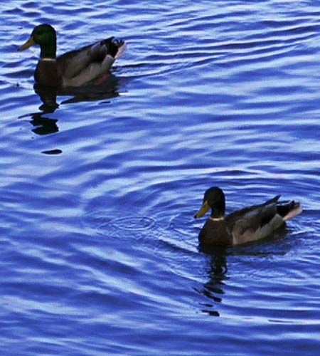
FARAMARZI et al.: BLIND SR OF REAL-LIFE VIDEO SEQUENCES                                                                                                1551

Fig. 5. Experimental results for the Mobile video sequence (please zoom into the figure on screen; see the videos at http://lyle.smu.edu/~rajand/Video_SR/).
(a) Ground-truth video frame. (b) One LR frame generated by applying a 9 × 9 motion blur with size of 15 × 15, spatial downsampling of 2, and Gaussian
noise with SNR of 30d B, then upsampled to the original resolution using Bicubic; (c) Original blur; (d) The reconstruction result of 3D-ISKR [38]
deblurred by [39] with PSNR of 31d B; (e) The reconstruction result of our proposed method with PSNR of 32.2d B; (f) The estimated PSF with
NMSE of 0.015.

               IV. F INAL HR F RAME E STIMATION                                 and the m-th diagonal element of Onk,i is computed              according
                                                                                to:
   After the PSF estimation is completed, the final HR frames                                      ⎧                                           ⎫
are reconstructed through minimizing the following cost                                            ⎨ Rm ρ(DHMk,i fkn−1 − gi )
                                                                                                                                                ⎬

function:                                                                           ok,i [m] = ex p −                                                 (22)
                                                                                                   ⎩               2σ 2                           ⎭
                           ⎛

                         P
                             k+N
                                                                            where in (22) Rm is a patch operator which extracts a patch
 J (f1 , . . . , f P ) =   ⎝     ρ Ok,i DHMk,i fk − gi
                                                           1                    of size q × q centered at the m-th pixel of fk,i .
                      k=1    i=k−M
                                                 ⎞                                 The final frame estimation procedure is demonstrated

                                  4
                                                                            in Algorithm 2.
                               +λ   ρ ∇ j fk  ⎠                        (19)                   V. E XPERIMENTAL R ESULTS
                                               1
                                     j =1
                                                                                   In this section, the performance of our method is evaluated
                                                                                and compared with the state-of-the-art video SR methods
where Ok,i is a diagonal weighting matrix that assigns less
                                                                                3D-ISKR4 [38] and Fast Upsampler [42] which are available
weights to the outliers. Minimizing this cost function with
                                                                                for public evaluation, and also with the commercial software
respect to fk yields:
                                                                                Video Enhancer [43]. Among these three, we only display the
 ⎛                                                                   ⎞          results from 3D-ISKR [38]. This non-blind SR method does

     k+N
                                                  4
                                                                                not include a debluring step, so we post process its outputs
 ⎝            T
             Mk,i HT DT Onk,i Vn DHMk,i + λ               ∇ Tj Wn ∇ j ⎠ fkn
                                                                                with the debluring method of [39]. Different parameters for
     i=k−M                                         j =1
                                                                                debluring were tried out in each experiment to get the best pos-
                                          T
                                       = Mk,i HT DT Onk,i Vn gi          (20)   sible outcomes from 3D-ISKR. Furthermore, since 3D-ISKR
                                                                                implementation does not estimate pixels near frame bound-
where:                                                                          aries, we remove the boundaries from the reconstructed frame
                                                                                before an objective evaluation. As the outputs of Fast Upsam-
                Vn = diag ρ(DHMk,i fkn−1 − gi ) ,                               pler and Video Enhancer have always a small global misalign-
                                                                                ment with the ground-truth frames, we use Keren method [44]
               Wnj = diag ρ(∇ j fkn−1 )                                  (21)    4 Iterative Steering Kernel Regression.
1552 IEEE TRANSACTIONS ON IMAGE PROCESSING, VOL. 25, NO. 4, APRIL 2016
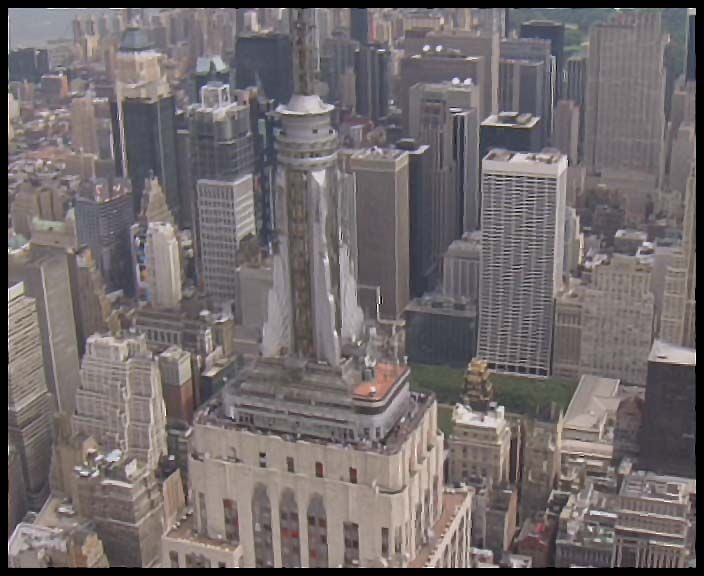
Fig. 6. Experimental results for some popular HD (1080p) video sequences with complicated motions; the frames are cropped for better visibility (please
zoom into the figure on screen; see the videos at http://lyle.smu.edu/~rajand/Video_SR/).The SR upsampling ratio and temporal window size are 2 and 5,
respectively. (a) BQ Terrace. (b) Crowd Run. (c) Old Town Cross. (d) Ducks Take Off.
to estimate and compensate the global misalignments. The by normalized mean square error (NMSE) defined as:
reconstructed videos of our proposed method are available
at http://lyle.smu.edu/~rajand/Video_SR/. h − ĥ2
NMSE(ĥ) = , (24)
To measure the accuracy of our proposed blind method h2
for different blur types, we synthetically generate LR video
sequences from four popular videos commonly used in where h and hÌ‚ ˆ are the original and estimated blurs, respec-
video processing experiments: City, Mobile, Foreman, and tively. The goal is to obtain high frame-PSNR and low
Bus. All these videos have 4:2:0 chroma subsampling for- PSF-NMSE values.
mat which means the chrominance channels have half of For the first experiment, the City video sequence (one frame
the horizontal and vertical resolutions of the luminance of which is shown in Fig. 3(a)) in 4CIF resolution is used.
channel [25]. The PSFs in the experiments are generated using It contains many structures at different scales, some of which
the MATLAB function fspecial(). Also we demonstrate the are smaller than the support of applied blur. This sequence
results of upscaling some other popular videos to the FHD5 is blurred by applying a Gaussian PSF of size 15 × 15
or 1080p (1920×1080 progressive) resolution. Furthermore, to with the standard deviation of 1.2, downsampled by a factor
see the performance for an actual video (i.e. not downsampled of 2, and corrupted by Gaussian noise with SNR of 30d B.
by our method), we use Highway video sequence to upscale The Bicubically-upsampled LR frame and the applied PSF
it from CIF (352 × 288) to 4CIF (704 × 576) resolution. are shown in Figs. 3(b) and (c), respectively. The size of
For objective evaluation of the frame reconstruction perfor- SR temporal window is 5 (with 2 frames forward and 2 frames
mance of the proposed method, we use peak signal-to-noise backward). To estimate the blur(s), the frames are first upsam-
ratio (PSNR) which is defined for the pixel intensity range of pled using the NUI method, then the luma channel of each
[0, 255] as: frame is smoothed out (Fig. 3(d)), its gradient magnitude is
f f calculated (Fig. 3(e)), and its salient edges not belonging to
2552 Nx N y C
PSNR(f̂) = 10 log10 , (23) structures finer than the kernel support are extracted (Fig. 3(f)).
f − f̂2 The reconstructed frame using 3D-ISKR [38] deblurred by [39]
ˆ are the ground-truth and reconstructed frames,
where f and f̂
is shown in Fig. 3(g) with PSNR of 28.9d B (after border
removal). The estimated HR frame and PSF using our
respectively. Also the accuracy of blur estimation is evaluated
method are shown in Figs. 3(h) and (i) with frame-PSNR of
5 Full High Definition. 32.4d B and PSF-NMSE of 0.01. Both subjective and object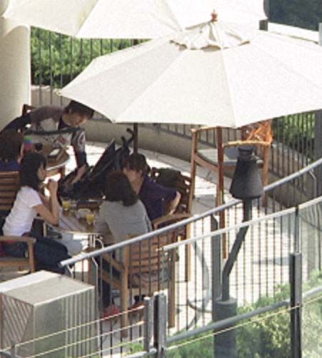
FARAMARZI et al.: BLIND SR OF REAL-LIFE VIDEO SEQUENCES 1553
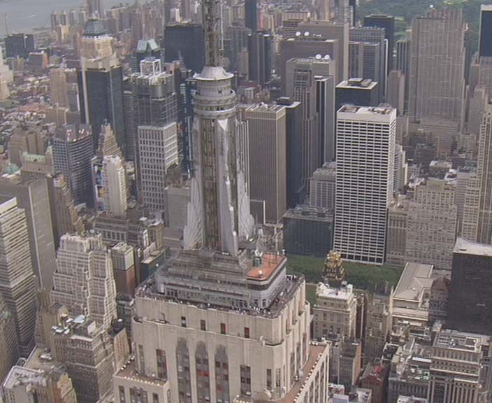
Fig. 7. (a) One frame of Highway video sequence; (b) The result of proposed method. The resolution is improved (e.g. see the green sign) and the noise is
reduced. Please see the video at http://lyle.smu.edu/~rajand/Video_SR/.
TABLE I Fig. 6 demonstrates the performance of our SR method
PSNR C OMPARISON B ETWEEN THE P ROPOSED M ETHOD versus Bicubic for some popular 1080p video sequences
AND THE S TATE OF THE A RT
having complicated motions. The resolution improvement is
clearly observable in all cases. The masking operation has
successfully suppressed motion artifacts in occluded regions
(e.g. around the runners) and deformable area (e.g. torch flame,
stream of water).
Now we evaluate the proposed method using a real-life low
quality and noisy video sequence. Fig. (a) displays one frame
of the Highway sequence in CIF resolution. This is a fast
comparisons confirm superiority of the proposed method over moving scene and so is challenging for SR processing. The
3D-ISKR. resulting 4CIF video using our proposed method is shown
For the second experiment, the Mobile sequence in CIF res- in (b). The resolution is visibly improved as can be seen
olution is chosen (Fig. 4(a)). This sequence is blurred by a 5×5 for instance from the green signboard. Also the noise level
out-of focus PSF with size of 15×15, downsampled by apply- is significantly suppressed.
ing a SR factor of 2 and contaminated by additive Gaussian
noise with SNR of 40d B. One Bicubically-upsampled LR VI. C ONCLUSION
frame and the original PSF are shown in Figs. 4(b) and (c), A method for blind deconvolution and super resolution
respectively. To reconstruct each HR frame, we use a window from one low-resolution video is introduced in this paper.
of length 5. Fig. 4(d) shows the reconstruction result of The complicated nature of motion fields in real-life videos
3D-ISKR [38] deblurred by [39] with PSNR of 21.2d B. make the frame and blur estimations a challenging problem.
Also, Figs. 4(e) and (f) demonstrate the estimated frame and To estimate the blur(s), the input frames are first upsampled
PSF using our method with frame-PSNR of 22.7d B and using non-uniform interpolation (NUI) SR method assuming
PSF-NMSE of 0.015. that the blurs are either identical or have slow variations over
As the third experiment, the Foreman video sequence time. Then the blurs are determined iteratively from some
(Fig. 5(a)) is blurred with a 45-degree motion blur of size enhanced edges in the upsampled frames. After completion of
15 × 15 with the support size of 9 × 9, downsampled by blur estimation, the reconstructed frames are discarded and a
a SR factor of 2, and contaminated by 30 dB noise. One non-blind iterative SR process is performed to obtain the final
Bicubically-upsampled LR frame and the PSF are presented reconstructed frames using the estimated blur(s). A masking
in Figs. 5(b) and (c), respectively. The reconstruction result operation is applied during each iteration of the final frame
of [38] is demonstrated in Fig. 5(d) with PSNR of 32d B. The reconstruction to successively suppress artifacts resulted by
reconstructed image and the estimated PSF obtained by our inaccurate motion estimation. Comparison is made with the
proposed method are shown in Figs. 5(e) and (f), respectively state of the art and the superior performance of our proposed
with PSNR of 33.1d B and NMSE of 0.08. method is confirmed through different experiments.
Table I summarizes the PSNR values from our method
compared to those from 3D-ISKR [38] (deblurred by [45]),
R EFERENCES
Video Enhancer [43], Fast Upsampler [42], and Bicubic for
different video sequences. In all experiments, the proposed [1] E. Faramarzi, V. R. Bhakta, D. Rajan, and M. P. Christensen, “Super
resolution results in PANOPTES, an adaptive multi-aperture folded
method outperforms other methods with significant PSNR architecture,” in Proc. 17th IEEE Int. Conf. Image Process. (ICIP),
differences. Sep. 2010, pp. 2833–2836.1554 IEEE TRANSACTIONS ON IMAGE PROCESSING, VOL. 25, NO. 4, APRIL 2016
[2] E. Faramarzi, D. Rajan, and M. P. Christensen, “Unified blind method [29] M. Elad and Y. Hel-Or, “A fast super-resolution reconstruction algorithm
for multi-image super-resolution and single/multi-image blur deconvo- for pure translational motion and common space-invariant blur,” IEEE
lution,” IEEE Trans. Image Process., vol. 22, no. 6, pp. 2101–2114, Trans. Image Process., vol. 10, no. 8, pp. 1187–1193, Aug. 2001.
Jun. 2013. [30] J. R. Shewchuk, “An introduction to the conjugate gradient method with-
[3] S. Borman and R. L. Stevenson, “Spatial resolution enhancement of low- out the agonizing pain,” School Comput. Sci., Carnegie Mellon Univ.,
resolution image sequences: A comprehensive review with directions for Pittsburgh, PA, USA, Tech. Rep. CMU-CS-94-125, 1994.
future research,” Dept. Elect. Eng., Univ. Notre Dame, Notre Dame, IN, [31] C. R. Vogel and M. E. Oman, “Iterative methods for total variation
USA, Tech. Rep., Jul. 1998. denoising,” SIAM J. Sci. Comput., vol. 17, no. 1, pp. 227–238, 1996.
[4] S. Borman and R. L. Stevenson, “Super-resolution from image [32] D. Krishnan, T. Tay, and R. Fergus, “Blind deconvolution using
sequences—A review,” in Proc. Midwest Symp. Circuits Syst., a normalized sparsity measure,” in Proc. IEEE CVPR, Jun. 2011,
Notre Dame, IN, USA, Aug. 1998, pp. 374–378. pp. 233–240.
[5] S. C. Park, M. K. Park, and M. G. Kang, “Super-resolution image [33] C. Wang, L. Sun, P. Cui, J. Zhang, and S. Yang, “Analyzing image
reconstruction: A technical overview,” IEEE Signal Process. Mag., deblurring through three paradigms,” IEEE Trans. Image Process.,
vol. 20, no. 3, pp. 21–36, May 2003. vol. 21, no. 1, pp. 115–129, Jan. 2012.
[6] R. R. Schultz, L. Meng, and R. L. Stevenson, “Subpixel motion [34] J. H. Money and S. H. Kang, “Total variation minimizing blind decon-
estimation for super-resolution image sequence enhancement,” J. Vis. volution with shock filter reference,” Image Vis. Comput., vol. 26, no. 2,
Commun. Image Represent., vol. 9, no. 1, pp. 38–50, Mar. 1998. pp. 302–314, 2008.
[7] A. M. Tekalp, Digital Video Processing (Prentice Hall Signal Processing [35] S. Osher and L. I. Rudin, “Feature-oriented image enhancement using
Series). Englewood Cliffs, NJ, USA: Prentice-Hall, 1995. shock filters,” SIAM J. Numer. Anal., vol. 27, no. 4, pp. 919–940, 1990.
[8] Y. Caspi and M. Irani, “Spatio-temporal alignment of sequences,” IEEE [36] C. Tomasi and R. Manduchi, “Bilateral filtering for gray and color
Trans. Pattern Anal. Mach. Intell., vol. 24, no. 11, pp. 1409–1424, images,” in Proc. 6th Int. Conf. Comput. Vis. (ICCV), Washington, DC,
Nov. 2002. USA, Jan. 1998, pp. 839–846.
[9] O. Shahar, A. Faktor, and M. Irani, “Space-time super-resolution from [37] N. Joshi, R. Szeliski, and D. Kriegman, “PSF estimation using sharp
a single video,” in Proc. IEEE Comput. Soc. Conf. Comput. Vis. Pattern edge prediction,” in Proc. IEEE Conf. Comput. Vis. Pattern Recognit.,
Recognit. (CVPR), Jun. 2011, pp. 3353–3360. Anchorage, AK, USA, Jun. 2008, pp. 1–8.
[10] V. Cheung, B. J. Frey, and N. Jojic, “Video epitomes,” Int. J. Comput. [38] H. Takeda, P. Milanfar, M. Protter, and M. Elad, “Super-resolution with-
Vis., vol. 76, no. 2, pp. 141–152, 2008. out explicit subpixel motion estimation,” IEEE Trans. Image Process.,
[11] R. Fergus, B. Singh, A. Hertzmann, S. T. Roweis, and W. T. Freeman, vol. 18, no. 9, pp. 1958–1975, Sep. 2009.
“Removing camera shake from a single photograph,” ACM Trans. [39] A. Levin, R. Fergus, F. Durand, and W. T. Freeman, “Image and depth
Graph., vol. 25, no. 3, pp. 787–794, 2006. from a conventional camera with a coded aperture,” ACM Trans. Graph.,
[12] Q. Shan, J. Jia, and A. Agarwala, “High-quality motion deblurring from vol. 26, no. 3, 2007, Art. ID 70.
a single image,” ACM Trans. Graph., vol. 27, no. 3, p. 73, 2008. [40] L. Xu, C. Lu, Y. Xu, and J. Jia, “Image smoothing via L 0 gradient
[13] S. Cho and S. Lee, “Fast motion deblurring,” ACM Trans. Graph., minimization,” ACM Trans. Graph., vol. 30, no. 6, 2011, Art. ID 174.
vol. 28, no. 5, 2009, Art. ID 145. [41] A. Levin, Y. Weiss, F. Durand, and W. T. Freeman, “Efficient mar-
[14] L. Xu and J. Jia, “Two-phase kernel estimation for robust motion ginal likelihood optimization in blind deconvolution,” in Proc. IEEE
deblurring,” in Proc. 11th Eur. Conf. Comput. Vis., 2010, pp. 157–170. Comput. Soc. Conf. Comput. Vis. Pattern Recognit. (CVPR), Jun. 2011,
[15] T. F. Chan and C.-K. Wong, “Total variation blind deconvolution,” IEEE pp. 2657–2664.
Trans. Image Process., vol. 7, no. 3, pp. 370–375, Mar. 1998. [42] Q. Shan, Z. Li, J. Jia, and C.-K. Tang, “Fast image/video upsampling,”
[16] Y.-L. You and M. Kaveh, “A regularization approach to joint blur ACM Trans. Graph., vol. 27, no. 5, 2008, Art. ID 153.
identification and image restoration,” IEEE Trans. Image Process., vol. 5, [43] Video Enhancer v1.9.10. [Online]. Available: http://www.infognition.
no. 3, pp. 416–428, Mar. 1996. com/VideoEnhancer/
[17] Y.-L. You and M. Kaveh, “Blind image restoration by anisotropic [44] D. Keren, S. Peleg, and R. Brada, “Image sequence enhancement using
regularization,” IEEE Trans. Image Process., vol. 8, no. 3, pp. 396–407, sub-pixel displacements,” in Proc. IEEE Comput. Soc. Conf. Comput.
Mar. 1999. Vis. Pattern Recognit. (CVPR), Jun. 1988, pp. 742–746.
[18] F. Šroubek and J. Flusser, “Multichannel blind deconvolution of spa- [45] A. Levin, Y. Weiss, F. Durand, and W. T. Freeman, “Understanding and
tially misaligned images,” IEEE Trans. Image Process., vol. 14, no. 7, evaluating blind deconvolution algorithms,” in Proc. IEEE Comput. Soc.
pp. 874–883, Jul. 2005. Conf. Comput. Vis. Pattern Recognit. (CVPR), Jun. 2009, pp. 1964–1971.
[19] F. Šroubek, G. Cristóbal, and J. Flusser, “A unified approach to super-
resolution and multichannel blind deconvolution,” IEEE Trans. Image
Process., vol. 16, no. 9, pp. 2322–2332, Sep. 2007.
[20] F. Šroubek, J. Flusser, and M. Šorel, “Superresolution and blind decon-
volution of video,” in Proc. 19th Int. Conf. Pattern Recognit. (ICPR),
Dec. 2008, pp. 1–4.
[21] C. Liu and D. Sun, “A Bayesian approach to adaptive video super
resolution,” in Proc. IEEE Conf. Comput. Vis. Pattern Recognit. (CVPR),
Jun. 2011, pp. 209–216.
[22] C. Liu and D. Sun, “On Bayesian adaptive video super resolution,”
IEEE Trans. Pattern Anal. Mach. Intell., vol. 36, no. 2, pp. 346–360,
Feb. 2014.
[23] E. Shechtman, Y. Caspi, and M. Irani, “Space-time super-resolution,”
IEEE Trans. Pattern Anal. Mach. Intell., vol. 27, no. 4, pp. 531–545,
Apr. 2005.
[24] H. Takeda and P. Milanfar, “Removing motion blur with space– Esmaeil Faramarzi received the B.S. and M.S.
time processing,” IEEE Trans. Image Process., vol. 20, no. 10, degrees from the Amirkabir University of Technol-
pp. 2990–3000, Oct. 2011. ogy, Tehran, Iran, in 2000 and 2003, respectively,
[25] I. E. Richardson, The H.264 Advanced Video Compression Standard. and the Ph.D. degree from Southern Methodist Uni-
New York, NY, USA: Wiley, 2011. versity, Dallas, TX, USA, in 2012. From 2003 to
[26] C. Liu, “Beyond pixels: Exploring new representations and applications 2008, he was a Research Faculty Member with the
for motion analysis,” Ph.D. dissertation, Dept. Elect. Eng. Comput. Sci., Iranian Research Institute for Information Science
Massachusetts Institute of Technology, Cambridge, MA, USA, 2009. and Technology, Tehran, where he managed several
[27] F. Šroubek and P. Milanfar, “Robust multichannel blind deconvolution research projects and developed automation software
via fast alternating minimization,” IEEE Trans. Image Process., vol. 21, for image analysis and text recognition of scanned
no. 4, pp. 1687–1700, Apr. 2012. university dissertations and books written in Farsi
[28] R. C. Hardie, K. J. Barnard, J. G. Bognar, E. E. Armstrong, and and Latin languages. He is currently a Staff Engineer with Samsung Research
E. A. Watson, “High-resolution image reconstruction from a sequence of America, Richardson, TX. He made some contributions to the Display
rotated and translated frames and its application to an infrared imaging Adaptation part of ISO/IEC Green MPEG Standard for energy-efficient video
system,” Opt. Eng., vol. 37, no. 1, pp. 247–260, 1998. consumption.FARAMARZI et al.: BLIND SR OF REAL-LIFE VIDEO SEQUENCES 1555
Dinesh Rajan received the B.Tech. degree in elec- Marc P. Christensen received the B.S. degree
trical engineering from IIT IIT, Madras, and the in engineering physics from Cornell University,
M.S. and Ph.D. degrees in electrical and computer in 1993, the M.S. degree in electrical engineer-
engineering from Rice University, Houston, TX. ing from George Mason University, in 1998, and
He joined the Electrical Engineering Department, the Ph.D. degree in electrical and computer engi-
Southern Methodist University (SMU), Dallas, TX, neering from George Mason University, in 2001.
in 2002, as an Assistant Professor, where he is From 1991 to 1998, he was a Staff Member and
currently the Department Chair and Cecil and Ida Technical Leader with the Sensors and Photonics
Green Professor with the Electrical Engineering Group (now part of Northrop Grumman Mission
Department. His current research interests include Systems), BDM. His work ranged from developing
communications theory, wireless networks, informa- optical signal processing and VCSEL-based optical
tion theory, and computational imaging. He received the NSF CAREER Award interconnection architectures, to infrared sensor modeling, simulation, and
for his work on applying information theory to the design of mobile wireless analysis. In 1997, he co-founded Applied Photonics, a free-space optical
networks. He is a recipient of the Golden Mustang Outstanding Faculty Award interconnection module company. His responsibilities included hardware
and the Senior Ford Research Fellowship from SMU. demonstration for the DARPA MTO FAST-Net, VIVACE, and ACTIVE-EYES
programs, each of which incorporated precision optics, microoptoelectronic
arrays, and micromechanical arrays into large system level demonstrations.
In 2002, he joined Southern Methodist University. He has contributed to
large industry/university consortia centered on integrated photonics, such
Felix C. A. Fernandes received the as the DARPA PhASER and CIPhER programs. He has co-authored over
M.S. (Hons.) degree in computer science 100 journal and conference papers. He holds two patents in the field of
from the University of Kansas, Lawrence, in 1997, free space optical interconnections, one pending in the field of integrated
and the Ph.D. degree in electrical engineering from photonics, and four pending in the field of computational imaging. In 2010,
Rice University, in 2001. His dissertation was on he was selected as the inaugural Bobby B. Lyle Professor of Engineering
directional, shift-insensitive, and complex wavelet Innovation and serves as the Dean Ad Interim of the Lyle School of
transforms with controllable redundancy. From Engineering. In 2008, he was recognized for outstanding research with the
2001 to 2005, he was a member of the Technical Gerald J. Ford Research Fellowship.
Staff with the Video and Image Processing Branch,
R&D Center, Texas Instruments, where he was
the official ISO/IEC delegate and contributed
to the standardization of MPEG-4. His research spanned image/video
codecs, transcoding, error resilience, and digital camera pipelines. From
2005 to 2009, he was with WiQuest Communications, an ultrawideband
startup, where he architected a proprietary video codec that was productized
as a wireless docking station by Toshiba in their Portege R400 laptop.
In 2009, he designed and implemented image/video algorithms with
Ambrado, a startup targeting HD codecs on a parallel processor in
Toshiba/Ikegami studio cameras. Since 2010, he has been a Director of
media-processing research and standardization with Samsung Research
America, Dallas. His team has developed and standardized new technology
for video coding and fingerprinting, image search, multimedia transport, and
energy-efficient processing. He holds 14 issued patents, several pending,
and over 40 publications in peer-reviewed journals and conferences. He is
the Co-Chair of the ISO/IEC Green MPEG AdHoc Group, an Editor of
the MPEG Green Metadata Standard, and a member of the Eta Kappa Nu
Engineering Honor Society.You can also read