Registration of PE Segment contour deformations in digital High-Speed Videos
←
→
Page content transcription
If your browser does not render page correctly, please read the page content below
Registration of PE Segment contour deformations
           in digital High-Speed Videos
                  – submitted to Medical Image Analysis –

  Michael Stiglmayr∗†              Raphael Schwarz‡              Kathrin Klamroth†
                  Günter Leugering†                Jörg Lohscheller‡

                                         Abstract
          Oncologic therapy of laryngeal cancer may necessitate a total excision
      of the larynx which results into loss of voice. Voice rehabilitation can be
      archived using mucosal tissue vibrations at the upper part of the esopha-
      gus which serve as substitute voice generating element (PE segment). The
      quality of the substitute voice is closely related to vibratory characteris-
      tics of the PE segment. By means of a high-speed camera the dynamics
      of the PE segment can be recorded in real-time. Using image processing
      the deformations of the PE segment are extracted from the image series
      as deforming contours. Commonly, the characterization of PE dynamics
      bases on the spectral analysis of the time varying contour area. However,
      this constitutes an integral approach which masks most of the specific
      dynamics of PE deformations.
          We present an algorithm that automatically registers one segmented
      frame of the video sequence to the next frame to derive discrete 2-D trajec-
      tories of PE vibrations. By concatenation of the obtained transformations
      this approach provides a total registration of PE segment contours. We
      suggest a mixed-integer programming formulation for the problem that
      combines an advanced outlier handling with the introduction of dummy
      points in regions that newly open up, and that includes normal informa-
      tion in the objective function to avoid unwanted deformations. Numerical
      experiments show that the implemented alternate convex search algorithm
      produces robust results demonstrated in two high speed recordings of la-
      ryngectomee subjects.
   ∗ Corresponding author. E-mail: stiglmayr@am.uni-erlangen.de; Tel: +49 9131 8528306;
FAX: +49 9131 8528126; Adress: Institute of Applied Mathematics, Martensstr. 3, 91058
Erlangen, Germany; http://www2.am.uni-erlangen.de/∼stiglmayr
   † Institute of Applied Mathematics, University of Erlangen – Nürnberg, partially supported

by DFG, Sonderforschungsbereich 603 subproject C11
   ‡ Department of Phoniatrics and Pediatric Audiology, University of Erlangen – Nürnberg,

supported by DFG, Sonderforschungsbereich 603 subproject B5

                                              1
1 Introduction
Depending on the stage and location of laryngeal cancer the surgical excision
of the larynx may be the only adequate oncologic therapy. At a so-called total
laryngectomy the malignancy is excised in conjunction with the larynx which
requires a separation of the trachea and the esophagus to prevent uncontrolled
mixing of breathing and swallowing Blom (2000). While the connection of the
upper esophageal sphincter with the pharynx is not affected, the upper end of
the trachea is sutured into the anterior skin of the neck. The artificial tracheal
opening at the neck is called tracheostoma and facilitates the vitally important
maintenance of respiration. Due to the disconnection of the trachea from the
pharynx and the loss of the larynx a total laryngectomy results into the loss of
voice which deeply affects the post-surgical social integration Eadie and Doyle
(2004).
Rehabilitation of voice can be achieved by exciting tissue vibrations within
the esophagus serving as substitute voice generator to compensate the function
of the excised larynx. It is achieved by means of a silicon shunt valve that recon-
nects the trachea to the oral cavity. The prothesis builds up an unidirectional
connection and permits air to pass from the trachea into the esophagus but pre-
vents food from being aspirated into the trachea Blom (2000). Fig. 1.1 shows
schematically the main principle of tracheoesophageal voice production. The
shunt valve redirects the airstream into the esophagus when the tracheostoma
is manually occluded during exhalation. At the upper part of the esophagus
the streaming air excites tissue vibrations including the scar between esophagus
and the pharynx which in turn modulate the airstream and generate the substi-
tute voice signal. On account of the location of the oscillating tissue the sound
emitting part of the esophagus is named pharyngo-esophageal segment, abbre-
viated PE segment. Finally as in normal voice production, the acoustical signal
reaches the vocal tract, gets filtered by its resonance cavity, and is emitted as
voice signal through the mouth Titze (1994).
In comparison with normal voice, the quality of tracheoesophageal voice is
significantly reduced which affects the quality of life of patients which under-
went a larnygectomy van As-Brooks et al. (2005). Thus, voice therapy plays a
major part within the oncologic rehabilitation following surgery Schuster et al.
(2004). Improvement of voice quality requires a comprehensive understanding of
the substitute voice generating process. The quality of tracheoesophageal voice
depends essentially on the vibration pattern of the PE segment. In order to in-
vestigate the relationship between PE vibrations and voice quality the vibrations
of the PE segment have to be analyzed during sound production (i.e., phona-
tion). For this purpose PE segment vibrations are investigated using endoscopic
high-speed video systems which enable an insight into its anatomical, morpho-
logical, and dynamic characteristics in real-time. Current high-speed camera
systems have a frame rate of 4000 Hz and a spatial resolution of 256 × 256 pixel
(High-Speed Endocam, Wolf Corp., Knittlingen, Germany). Simultaneously,
the emitted acoustic signal is recorded (microphone: type B&K 4129 Brüel &
Kjaer Corp., sampling rate 44.1 kHz, discretization 16 bit).
2Microphone
Camera
d
a
a - Shunt valve
c b - Trachea
b c - Esophagus
d - PE segment
Figure 1.1: Principle of tracheoesophageal voice production. A tracheal
airstream passes through the shunt valve (a) and excites soft tissue vibrations
of the PE segment (d) which serves as substitute voice generating element.
A schematic draft of the examination situation is shown in Fig. 1.1. The
patients are instructed to articulate a vowel /a/ in a comfortable way. The
vibrations of the PE segment are recorded from a top-view position with a
high-speed camera system which is coupled to a rigid endoscope. Fig. 1.2 shows
short sequences of two high-speed recordings (A,B).
Within the sequences the deformations of the PE segment are captured. In
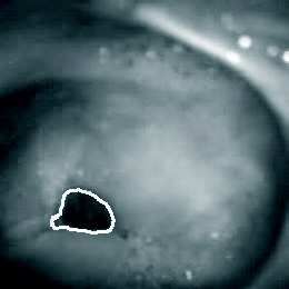
each frame the mucosal tissue of the PE segment forms a constriction within
the esophagus which constitutes the border of the enclosed opening. The visible
opening formed by the PE segment is called pseudoglottis. The two high-speed
movies show that the movements of the PE segment follow a quasi-periodic
vibration pattern. However, the PE segment oscillations of different subjects
diverge with respect to the shape, size, frequency, and orientation of pseudoglot-
tal deformations.
For the extraction of PE dynamics an image processing procedure had been
developed which bases on active contour models using an adapted gradient
vector flow field (GVF-field) as external force Lohscheller et al. (2004, 2003).
Fig. 1.3 shows the segmentation results of the high-speed movies A and B.
The contours track the deformation of the pseudoglottis and confirm the quasi-
periodic vibration characteristic of the PE segment.
By setting the spectral information of the pseudoglottal deformations into re-
lation to the spectral properties of the emitted acoustical signal the interrelation
between the substitute voice and the PE vibration could be verified Lohscheller
3pseudoglottis PE tissue
A
t = 0 ms t = 1 ms t = 2 ms t = 3 ms t = 4 ms
PE tissue
pseudoglottis
B
t = 0 ms t = 1.5 ms t = 3 ms t = 4.5 ms t = 6 ms
Figure 1.2: Oscillation cycles extracted from two high-speed movies (A,B)
recorded during sustained phonation of a vowel. The fundamental frequencies
of PE segment vibrations are 166 Hz and 125 Hz.
et al. (2004); Schuster et al. (2005). Up to now, just the time-varying pseu-
doglottal area function is derived from the segmentation results and serves as
measure to describe PE segment oscillations. As the analysis of the pseudoglot-
tal area is an integral approach, the specific information of the properties of the
PE tissue vibrations as oscillation directions, velocities and amplitudes gets lost.
Also no predictions can be made how to alter the PE morphology by surgical
intervention to modify the PE vibration pattern to improve voice quality.
In this work we propose a novel approach to register consecutive contours of
the PE segment in order to transfer the segmented contours into 2-D trajectories
of discrete contour points. This enables the formulation of an adequate objective
function and gives a detailed description of PE vibrations which is essential to
reveal the dynamics of PE segment vibrations.
A variety of different algorithms that use point alignment to find an opti-
mized transformation from a template image to a reference image have been
suggested in the recent literature. However, most of these methods have dif-
ficulties if applied to PE oscillations. For a proper registration of PE contour
deformations the following properties of PE oscillations are considered. Firstly,
data points of the PE segment are located on a single closed contour, and they
are consecutively numbered along this contour. Consequently, gradient informa-
tion can be approximated and incorporated into the the optimization process.
Secondly, the size and shape of the PE contours varies considerably during an
oscillation cycle. Thus, one-to-one point assignments are in general not suitable
to map contours from one frame to the next frame. This motivates the suggested
advanced outlier handling as well as the introduction of ’dummy points’ in re-
gions where new parts of the contour in the reference frame have no appropriate
counterpart in the template frame. Finally, information is used that a given PE
contour appears again after a certain time interval. Thus, correlating PE con-
4A
t = 0 ms t = 1 ms t = 2 ms t = 3 ms t = 4 ms
B
t = 0 ms t = 1.5 ms t = 3 ms t = 4.5 ms t = 6 ms
Figure 1.3: Segmentation results displayed within the oscillation cycles of high-
speed movies recorded from two male laryngectomees (A,B) during phonation.
The white lines mark the segmented contours of the pseudoglottis.
tours can be registered across an oscillation cycle which leads to a reduced error
propagation in contrast to an exclusive frame-by-frame registration.
The paper is organized as follows: After a brief review of the relevant lit-
erature in the following section, an advanced contour matching approach for
PE segment registration is described in Section 2.1. Results are discussed in
Section 3, and the paper is concluded in Section 4 with a short summary of the
results and an outlook on further research tasks.
1.1 Literature review
The following brief literature review concentrates on point based registration ap-
proaches that appear to be suitable for PE segment registration, and discusses
their advantages as well as their shortcomings in the context of the applica-
tion at hand. Since the suggested adaptive contour matching approach extends
ideas from the robust point matching method of Chui and Rangarajan (2003),
the corresponding results are reviewed in more detail.
The strategy using the obtained registration function as an approximation
of the sought physical movement is already mentioned and used in Saadah et al.
(1998) for the movement of the local folds in the larynx. The difference between
our model and the model used in Saadah et al. (1998) is that we restrict the
function space of the sought registration function, whereas in Saadah et al.
(1998) a priori every two dimensional vector field u(x) is thought of as a possible
movement f (x) = x + u(x). To ensure a certain degree of ”smoothness”, the
angle between the displacement vectors of consecutive points on the contour
is used as a regularization term. But with a movement described by a vector
field no evaluation of the registration function outside of the considered points
5is possible. Therefore the gained information is very limited. We are going to
present a method that overcomes these drawbacks because the solution obtained
with this method is restriced to a ”nice” function space.
This is achieved by an extension of the following registration algorithms.
Landmark based registration algorithms like those suggested, for example, in
Banerjee et al. (1995) use invariants of rigid transformations (such as angles or
parallel lines) to find corresponding points (landmarks) in the reference and in
the template image. Alternatively, landmarks can be selected manually (for ex-
ample, by the physician) or automatically together with their correspondences.
In medical image registration, morphologically characteristic landmarks can be
used and automatically detected in both images. Consequently, landmark based
algorithms are in most cases specialized to specific registration tasks, see Betke
et al. (2003). Even though there are extensions to landmark based registra-
tion algorithms to non-rigid transformations like in Johnson and Christensen
(2002) the problem of finding correspondances remaines. Therefore landmark
based registration algorithms are not suitable for our purpose. Moreover, it
is generally impossible to decide how the data points are shifted between two
consecutive frames of the video sequence since the movement of the soft tissue
in the PE segment is to an extreme degree non rigid.
The iterative closest point algorithm (ICP) first proposed in Besl and McKay
(1992) uses a heuristic to find corresponding points. Each point in the first image
is assigned to the nearest point in the second image, and the transformation
is computed such that the sum of squared distances (SSD) between assigned
points is minimal. This procedure is iterated until no further improvement of
the SSD can be achieved. For rigid transformations, and given a good starting
solution, this method works well and produces stable results. However, if non-
rigid transformations are sought, or if a good initial guess is not available, the
ICP generally converges to a stationary point or local minimum, which may in
fact be far away from a reasonably good solution. There are various variants
and improvements of the ICP, some of them are listed in Liu (2004).
In addition to the fact that the PE segment moves non-rigidly we have to
address the problem of outlier points. The number of points on the contour
may largely vary between consecutive frames because of the different contour
length. This typically happens, for example, if the PE segment opens up in
an area where it was previously closed and thus not visibly for the camera.
In this situation a one-to-one point assignment is not meaningful. Note that
this problem can not be overcome with a simple re-sampling step since the
foregoing segmentation based on active contours (snakes) generates in general
non-uniformly distributed points on the contour.
Chui and Rangarajan (2003) propose a robust point matching algorithm that
incorporates a strategy for outlier handling in an ICP framework. The method
is based on the formulation of a generalized assignment problem for finding
corresponding points, and it involves the optimization of two types of variables:
Discrete (binary) assignment variables and continuous transformation variables.
Since our approach is closely related to the robust point matching algorithm, it
will be reviewed in the following.
6Problem 1.1 (Chui and Rangarajan (2003)). Let X = {x1 , . . . , xI } and Y =
{y1 , . . . , yJ } be sets of points in the template and the reference image, respec-
tively, and let F be a finite dimensional function space containing candidates for
the sought transformation f between X and Y . Then the robust point matching
problem can be formulated as
J
I P J
I P
P 2 2 P
min zij kyj − f (xi )k + λ kLf k − ξ zij
i=1 j=1 i=1 j=1
PI+1
s.t. i=1 zij = 1 ∀j ∈ {1, . . . , J}
PJ+1 (1.1)
j=1 zij = 1 ∀i ∈ {1, . . . , I}
zij ∈ {0, 1} ∀i ∈ {1, . . . , I +1} ∧ j ∈ {1, . . . , J +1}
f ∈ F,
2
where λ, ξ ≥ 0 are fixed penalty parameters and kLf k is a measure for the
smoothness of the transformation function f ∈ F.
In formulation (1.1), the assignment variables zij , i ∈ {1, . . . , I}, j ∈ {1, . . . ,
J}, are equal to 1 if the point xi is assigned to the point yj , and 0 otherwise.
2
Thus the product zij kyj − f (xi )k in the objective function implies the min-
2
imization of the distance kyj − f (xi )k only for those pairs of points yj and
f (xi ) that are assigned to each other. If zi,J+1 = 1 for some i ∈ {1, . . . , I} or
if zI+1,j = 1 for some j ∈ {1, . . . , J}, the point xi or yj , respectively, is con-
sidered as an outlier and is excluded from the P distance
PJminimization. To avoid
I
solutions with too many outliers, the term −ξ i=1 j=1 zij is included in the
objective function, where ξ ∈ R+ is a steering parameter that can be adapted
with respect to the specific problem at hand. The smaller ξ becomes the more
points are identified as outliers, and in the case of ξ = 0 it is always optimal to
consider every point as an outlier.
The function space F in (1.1) may be based on thin plate splines or radial
basis functions, or it may be restricted to affine or rigid mappings. It should
be noted that even if improvements of the ICP are applied to problem (1.1), it
is very difficult or in some cases even impossible to find a global or even local
optimum of the robust point matching problem for general non-rigid transfor-
mations.
But also for ’simple’ function spaces F, solving the robust point matching
problem (1.1) remains computationally expensive. Due to the combination of
integer assignment and continuous function interpolation variables, it belongs
to the class of mixed integer programming problems (MIP), for which no poly-
nomial time algorithm is known in general.
To overcome this difficulty, Chui and Rangarajan (2003) suggest a heuristic
solution approach similar to the ICP, which solves the problem iteratively in
the discrete and in the continuous variables. The resulting subproblems are
an integer linear programming problem (in the assignment variables zij ) and a
convex optimization problem (in the transformation function f ).
Note that due to the structure of the constraints the assignment matrices
are contained in a polytope whose edges are binary matrices, as also noted in
7Rangarajan et al. (1997a). The assignment subproblems are therefore totally
unimodular, which implies that the assignment subproblem of (1.1) always has
an integer optimal solution, even if the integrality constraints are relaxed to
zij ∈ [0, 1] ∀i ∈ {1, . . . , I + 1}, j ∈ {1, . . . , J + 1}.
The main drawback of this approach if applied to PE segment registration
can be seen in the fact, that only the position of the points is taken into ac-
count, and no information about the shape of the contour is used. Numerical
experiments showed that this often leads to wrong correspondences in the video
frames, especially when the contour of the PE segment closes and opens again.
In most of these cases we obtained assignments of points that are located on
opposite sides of the gap. Due to these wrong assignments the corresponding
transformations f may be strange functions with (locally) very large gradients.
Another modell formulation for the point matching problem is proposed
by Zheng and Doermann (2006). An assignmet is there choosen such, that
neighbooring structures are preserved and the mapping is “locally rigid”. But
this may lead to arbitrary mappings and the movement of the PE Segment is
not “locally rigid”.
This motivates the formulation of an alternative, adaptive contour matching
problem and -algorithm that is capable of separating opposite contour lines, and
that effectively uses all the information available in PE segment registration.
2 Methods
2.1 Registration of consecutive PE contours
While motivated by - and based on - the robust point matching algorithm of
Chui and Rangarajan (2003), the adaptive contour matching approach described
below modifies and extends this method in various ways to better incorporate
the problem structure and the characteristics of PE segment registration. An
advanced outlier handling, allowing for asymmetric assignments and dummy
point introduction, is combined with an enhanced problem description incor-
porating gradient information. Particularly, introducing knowledge about the
temporal properties of PE contour deformations facilitates proper registration
results. The proposed registration procedure is also well suited for further regis-
tration problems that are based on a preceding segmentation step which yields
finite and ordered point sets along closed contours.
2.1.1 Including normal information
One of the most problematic situations in PE segment registration is the reg-
istration of contours with incisions. When the distance between opposite curve
segments of the contour is small, the robust point matching algorithm of Chui
and Rangarajan (2003) frequently generates assignments across the shape (more
or less independently of the chosen parameter settings). Measuring the regis-
tration error exclusively based on squared Euclidean distances between corre-
sponding points is therefore not sufficient in this case. Therefore, we suggest
8to use additionally a different quality measure, that is easily computable, that
allows the separation of the inside from the outside of the contour, and that
provides information about the local shape of the contour. These requirements
are met, for example, by the angle between the normal vectors n(y) to the con-
tour, which can be easily approximated at the individual data points y = yj ,
j = {1, . . . , J} using the two adjacent data points yj−1 and yj+1 that are im-
mediately available due to the fixed ordering of points along the contour, see
Figure 2.1.1. (To simplify notation, we set yJ+1 = y1 and xI+1 = x1 .)
.
t(yj ) .......
q
....... ..
....... ..
yj+1
....... .
kt(yj )k
..........
....
.......
.......
....
...
.
...... ...... ...
............ .... . ............
. ..
...
......... ........ ......... ....... ..
. . ..
.......... .. ....... ..
·q ...
n(y )
j
.....
...... ................
........... ..
........... ...
... ..... ....................
...
y
... j ... .........
·
..... ...
.. ........
.... .. .. ..
......
...
... ... ......
... .. ..
... .. ......
..
... ... ......
... . ..
.... .
..
.
.. .
... ....
...
....
q .....
yj−1
Figure 2.1: Approximation of the normal vector n(yj ) and of the normalized
t(y )
tangent vector kt(yjj )k at yj
The additional integration of normal information, as also mentioned in Fry
(1997), leads to a model formulation that considers both the local topology of
the shape and the Euclidean distance between corresponding points. Unlike Fry
(1997) who uses normal information as a distance measure for shape recognition,
we want to augment the registration process with this concept.
Since the angle α between two normal vectors n(yj ), n(f (xi )) is equal to the
angle between the corresponding tangent vectors t(yj ), t(f (xi )), the normal-
angle-distance between two points f (xi ) and yj , i = {1, . . . , I}, j = {1, . . . , J}
can be approximated as follows:
T
(f (xi+1 ) − f (xi−1 )) (yj+1 − yj−1 )
dN
ij = 1 − cos α = 1 − . (2.1)
kf (xi+1 ) − f (xi−1 )k kyj+1 − yj−1 k
The relative influence of the normal distance as compared to the influence
of the Euclidean distance in the objective function is controlled via a weighting
9parameter δ ∈ [0, 1]. This yields the following modified objective function:
X J
I X X J
I X X J
I X
min δ zij dij + (1 − δ) zij dN
ij − ξ zij , (2.2)
i=1 j=1 i=1 j=1 i=1 j=1
2
where dij = kf (xi ) − yj k is the Euclidean distance between the points yj and
f (xi ), i = {1, . . . , I}, j = {1, . . . , J}. This formulation has an interesting inter-
pretation from the point of view of multicriteria optimization, where two or more
objectives are optimized simultaneously. For all values of δ ∈ [0, 1], objective
(2.2) can be seen as a weighted sums scalarization combining the two individual
PI PJ PI PJ
criteria i=1 j=1 zij dij and i=1 j=1 zij dN ij into one joint objective func-
PI PJ
tion. Similarly, the term i=1 j=1 zij can be interpreted as a third objective
aiming at the rejection of solutions with too many outliers, and weighted with
the parameter −ξ. The resulting optimization problems are well posed for all
feasible choices of δ and ξ, and they all yield a feasible registration. However,
the registration result does for some parameter settings meet the requirements
of the application in PE segment registration more than for others, even though
we cannot define a ’best choice’ for the parameters δ and ξ from a theoretical
point of view. In the computational tests a parameter δ = 0.85 provided good
results. Since the effect of the parameter ξ is to a high degree dependent of the
distance l between consecutive points on the contour, we selected ξ relative to
l.
2.1.2 Asymmetric assignments: An alternative outlier
handling
Different effects can corrupt the image quality during image acquisition, and
wrong point detection may be a consequence of the segmentation procedure. To
avoid that wrongly segmented points disturb the registration result, they should
be identified as outliers and hence not taken into account when computing the
transformation function. In this context, several authors suggested preprocess-
ing steps using statistical methods for outlier rejection, see, for example, Besl
and McKay (1992) and Wells III (1997), or special metrics that restrict the
influence of outliers, Mount et al. (1998). Including a term for outlier handling
directly in the assignment problem was suggested by Rangarajan et al. (1997b),
and in a similar form by Zhang (1994) for free-form surfaces. This approach pro-
vides a comparably robust and elegant method that achieves good registration
results even in the case of data or segmentation errors.
In PE segment registration we have a different situation. Due to the rela-
tively clear structure of the PE segment with clearly visible boundaries in the
video frames, the segmentation yields in general good results and there is no
need to consider outliers caused by segmentation errors. However, in this case
we are confronted with a different kind of ’outliers’. The contour of the PE seg-
ment may be – and is in practice – often of varying length. Therefore the number
of detected points largely varies from frame to frame. Since between two frames
10with a different number of points no one-to-one correspondence exists, a new
kind of outlier handling has to be developed. Unlike the outliers caused by data
errors, these ’outliers’ should not be rejected during the registration process,
but used instead as additional information defining the contour. This motivates
the replacement of the classical assignment constraints in formulation (1.1) by
the following constraints for an asymmetric and ambiguous assignment
I
P
zij ≤ B1
i=1
PJ (2.3)
zij ≤ B2
j=1
with problem dependent and adaptable right hand sides B1 , B2 ≥ 1. We suggest
to select B1 and B2 depending on the ratio JI between the number of points in
the two frames that have to be registered. If I is significantly larger then J (for
example, if I > 1.1 · J), each data point yj , j = {1, . . . , J} may principally be
assigned to more than one data point xi , i = {1, . . . , I}. This can be realized,
for example, by setting B1 = 2 and B2 = 1. However, in order to get more
flexibility in the optimization process and thereby the ability to compensate
for the fact, that the points are in general not uniformly distributed along the
1
contour, we set B1 = B2 = 2 whenever 1.1 ≤ JI ≤ 1.1, i.e.,
1 if J > 1.1 · I 1 if I > 1.1 · J
B1 = B2 =
2 otherwise 2 otherwise.
By using inequality constraints in (2.3) (instead of equality constraints as in
the original assignment constraints, c.f. (1.1)), we can omit the outlier compo-
nent in the assignment matrices (i.e., the (I +1)-st and (J +1)-st row and col-
umn, respectively). Nevertheless, the penalty term or, to be more precise, the
PI PJ
’gratification term’ −ξ i=1 j=1 zij (c.f. (2.2)) is still needed in the objective
function since otherwise the ’empty’ assignment with zij = 0 ∀i ∈ {1, . . . , I},
j ∈ {1, . . . , J} would always be an (unwanted) optimal solution to the problem.
As in the robust point matching problem (1.1), the number of outliers can be
controlled by the parameter ξ. Its effect depends, among others, on the distance
between pairs of adjacent points in each data set (Euclidean plus normal-angle-
distance). Since, due to the relative benefit of assignment and non-assignment
in the objective function, only pairs of points with a combined distance smaller
than ξ are aligned in an optimal solution, we select the parameter ξ depending
on the magnitude of these point to point distances.
The discussion above leads to the following overall model for adaptive con-
11tour matching:
J
I P J
I P J
I P
zij dN
P P P
min δ zij dij + (1 − δ) ij − ξ zij
i=1 j=1 i=1 j=1 i=1 j=1
2
s.t. dij = kf (xi ) − yj k
(f (xi+1 )−f (xi−1 ))T (yj+1 −yj−1 )
dN
ij = 1 − kf (xi+1 )−f (xi−1 )kkyj+1 −yj−1 k (2.4)
PI
i=1 zij ≤ B1 ∀j ∈ {1, . . . , J}
PJ
j=1 zij ≤ B2 ∀i ∈ {1, . . . , I}
zij ∈ [0, 1] ∀i ∈ {1, . . . , I} ∧ j ∈ {1, . . . , J}.
Registration results based on formulation (2.4) for different outlier handling
parameters ξ are depicted in Figure 2.1.2.
2.1.3 Insertion of dummy points
As illustrated by the example in Figure 2.1.2, enforcing a complete registra-
tion with very few outliers may produce unrealistic transformations if the two
considered frames are rather different. From a theoretical point of view, the reg-
istration shown in Figure 2.1.2(c) may nevertheless be optimal: It contains only
very few outliers, and the distances between corresponding points are small.
On the other hand, one of the requirements for the transformation was, that it
should model the movement of the soft tissue in the PE segment. The function
shown in Figure 2.1.2(c) clearly does not meet this requirement.
In this example, the points in the two data sets do not represent the same
morphological situation. In other words, the points, that are visible in the first
frame, have not moved to cover all points in the second frame, and thus not
according to the transformation shown in Figure 2.1.2(c). In fact, another gap
has opened up in the PE segment that is visible in the second frame, but that
was not visible in the first frame. The points on the contour of the new gap
are in this sense ’new’ points that have no correspondence in the first frame.
Consequently, the movement of the left part of the segment that is present in
both frames is better represented by the transformation function found with a
smaller value of ξ as illustrated in Figure 2.1.2(b).
To obtain a realistic registration function that also simulates the movement
of points in the case that a new gap opens up in the PE segment, we suggest
the introduction of dummy points. Dummy points are artificial points that are
included as correspondences for the new points in a new part of the segment.
Allowing for ’pseudo assignments’ (i.e., assignments including dummy points),
information about the movement of the soft tissue at newly opened gaps can be
included in the model.
A first step towards this goal is to formulate criteria for the detection of
new gaps between two consecutive frames. This is realized by restricting the
total number of consecutive outliers, and evaluating the obtained registration
quality. If more than k consecutive points on the contour (with an appropriate
12(a) The template and the reference contour
before registration
y y
f(x) f(x)
(b) Small ξ (c) Larger ξ, with an additional contraint to
overcome the first local minimum
Figure 2.2: Registration results based on formulation (2.4) for different outlier
parameters ξ (frame 4)
parameter k > 0) are selected as outliers in an optimal solution of problem (2.4),
we can assume that a new gap in the contour has opened up. The parameter k
should be selected depending on the number of points in each frame, I and J.
For our data sets with 80 to 300 data points a choice of k ∈ [10, 15] led to the
best results.
In the following discussion we assume that the points yj , . . . , yj+κ are outliers
with some constant κ > k and that a good pre-registration is known (e.g., from
a previous registration step with a small value of ξ or, as sufficient in the case
of PE segment registration, given by the identity mapping).
Along the line starting from the centroid S of the κ outlier points in Y
and ending at the (closest) point x̄ = mini kS − xi k, we insert κ dummy points
x̃1 , . . . , x̃κ .
In every step two dummy points are placed, one of them shifted by a distance
13y
f(x)
qxL
......
......
......
......
......
...... .... q
........
ε
......
......
......
q ......
......
...... q
......
......
......
......
q ......
......
......
......
...
qS
Figure 2.3: Inserting dummy points (frame 4)
Figure 2.4: Re-registred with inserted dummy points (frame 4)
of ε to the left side of the line, the other to the right side. This is done in order
to allow for registration functions that separate the dummy points and aligns
them to opposite sides of the new contour. Using this approach, the tissue
movement can be simulated very well by the obtained registration function.
2.1.4 Alternate convex search algorithm
Problem (2.4) is strongly non-convex and has in general a very large number of
local minima, some of which correspond to very unrealistic registration functions
(c.f. Figure 2.1.2(c) for an example). The determination of a global optimum
with, for example, Branch and Bound methods is however in general very time-
consuming. Since each video sequence of the PE segment consists of several
hundreds of images that need to be registered, and since in this application the
identity mapping is a very good starting solution, we have instead implemented
a computationally efficient heuristic solution method based on ’Alternate Con-
vex Search’ (ACS). The method alternates between the determination of an
optimal assignment for a given (and fixed) transformation function f , and the
14consecutive optimization of f for the fixed assignment determined before. This
approach is iterated until no further improvements are made, or until some other
stopping condition is satisfied. Note that both subproblems (the optimization of
f for given z, and the optimization of z for given f ) are convex and can thus be
solved using methods of convex (or even linear) optimization. For the function
space F, from which the transformation function f has to be selected, we have
used thin-plate-splines as in Chui and Rangarajan (2003). The regularization
2
term kLf k is based on the gradients of the transformation functions f . For
a review of thin-plate splines and radial basis functions in image warping see
Modersitzki (2004), Rohr et al. (2001) or Arad and Reisfeld (1995). Summa-
rizing the discussion above, we can formulate an ’Adaptive Contour Matching’
algorithm as follows:
Algorithm 2.1 (Adaptive Contour Matching).
1. Set λ = λ0 > 0, ξ > 0, k ∈ N+ , 0 < τ < 1, 0 ≤ δ ≤ 1
2. Optimize zij with respect to
J
I P J
I P J
I P
zij dN
P P P
min δ zij dij + (1 − δ) ij − ξ zij
i=1 j=1 i=1 j=1 i=1 j=1
2
s.t. dij = kf (xi ) − yj k
(f (xi+1 )−f (xi−1 ))T (yj+1 −yj−1 )
dN
ij = 1 − kf (xi+1 )−f (xi−1 )kkyj+1 −yj−1 k
PI
i=1 zij ≤ B1 ∀j ∈ {1, . . . , J}
PJ
j=1 zij ≤ B2 ∀i ∈ {1, . . . , I}
zij ∈ [0, 1] ∀i ∈ {1, . . . , I} ∧ j ∈ {1, . . . , J}
3. Optimize f with respect to
J
I P
P 2 2
min zij kf (xi ) − yj k + λ kLf k
i=1 j=1
s.t. f ∈ F
4. WHILE no termination condition is satisfied, set λ = τ λ, GOTO (2)
5. IF κ > k consecutive points yj , . . . yj+κ are identified as outliers, GOTO (6),
ELSE STOP
6. Determine the centroid S of the κ consecutive outlier points
7. Determine x̄ = argminx∈X kS − xk
8. Insert κ points x̃1 , . . . , x̃κ along the line (S, x̄) as illustrated in Figure 2.1.3
9. Set X = X ∪ {x̃1 , . . . , x̃κ } and reorder the data points
10. GOTO (2)
152.2 Registration of periodic contour deformations
Processing an entire high-speed sequence demands the registration of several
hundreds of consecutive PE contours. A simple frame by frame registration
would cause serious error propagation which would finally lead to a complete
registration failure. However, PE contour deformations are not chaotic but
follow a quasi-periodic vibration pattern. Particularly, consecutive oscillation
cycles show strong geometric similarities of the deforming PE contours. Thus,
a certain PE geometry reoccurs after a certain time interval which depends on
the fundamental frequency of PE vibrations. Registration of PE contour defor-
mations takes advantage of the quasi-periodic PE vibration pattern. Initially,
for a high-speed sequence the fundamental frequency and cycle length of PE
vibrations is determined. Following, the entire sequence is decomposed into
consecutive cycles. Fig. 2.2 shows a PE oscillation cycle and schematically the
further registration process. The beginning and ending of a cycle is defined by
the maximum area (open-state) of the PE segment. The open-state possess a
high amount of contour points which positively influences the performance of
registration. Due to the knowledge that the last frame of a cycle resembles
the first one, the two images are initially registered across the oscillation cycle.
Following, starting from the first and last frame the remaining images of the PE
cycle are forward and reversely registered, respectively.
The intermediate image of a PE cycle is registered twice. For this image,
the analysis of differences between the forward and reverse registration enables
an objective error estimation for PE registration.
K
1 X f
err = y − yjr , (2.5)
K j=1 j 2
with K being the number of trajectories, yjf the endpoint of the jth trajctory
in the intermediate frame after forward registration and yjr the endpoint in the
intermediate frame after reverse registration.
For all consecutive oscillation cycles the procedure is iterated which leads to a
registration of an entire high-speed sequence.
2.3 Trajectories of discrete contour points
To visualize and validate the results of the obtained registration functions 2-D
trajectories of discrete contour points can be computed. Therefore, a sequence
of registrations over one oscillation cycle has to be computed. In the first frame
we select points on the contour line of the PE segment as starting points for
the tracing. After the computation of the registration function we apply it on
the selected points. In order to avoid error propagation we project the mapped
point orthogonally onto the contour line in the second frame. Since we select the
considered oscillation cycle such that the PE segment is opened in the starting
(and in the end) frame and (nearly) closed at a frame in the middle, the influence
of errors can be diminished by changing the order of registrations. Instead of
16initial cross cycle registration
open-state open-state
t = 0 ms t = 2 ms t = 4 ms t = 6 ms t = 8 ms
forward registration dual registration reverse registration
error estimation
Figure 2.5: Scheme for the registration of quasi-periodic PE contour defor-
mations. Error propagation is reduced by an initial cross cycle registration,
followed by successive forward/reverse registration steps. For the intermediate
frame the comparison of the two registration results enables an error estimation
of PE contour registration.
registering each frame to its consecutive frame, we determine the frame with the
smallest open PE segment and register forward before and backwards after it.
With this strategy the error made by merging the two parts of each trajectory is
smaller than the error propagation made by simple forward registration, because
the contour in the middle is smaller or even closed.
Algorithm 2.2 (Compute trajectories).
1. Choose an oscillation cycle, such that the PE segment is opened in the
starting frame st_frame and in the end frame end_frame. Determine the
frame m_frame with the smallest opening.
2. Select the starting points x1, . . . xn of the trajectories.
3. Register every frame from st_frame to m_frame −1 with its consecutive
frame according to algorithm 2.1.
4. Trace the selected points in st_frame using the obtained registration func-
tions.
5. Register st_frame to end_frame and compute the points corresponding
to x1, . . . xn in end_frame.
6. Register every frame from end_frame to m_frame +1 with its prior frame
according to Algorithm 2.1.
7. Trace the corresponding points in end_frame using the obtained registra-
tion functions.
173 Results and Discussion
3.1 Registration of consecutive PE contours
All of the computations presented in this section have been run on an Intel
Pentium 4, 2×3.2Ghz, 1000 MB RAM computer. The solution method was
implemented in Matlab. All results were found by one single computation,
using the identity mapping as starting solution for the transformation function
f . Since the implemented ACS method generally converges to a local minimum
in some attraction area of the starting solution, the results may vary if the
computations are repeated with different starting solutions.
y y
f(x) f(x)
Figure 3.1: Registration of frame 303 to frame 304 (parameter setting: ξ =
0.21629, δ = 0.85, λ0 = 0.001, τ = 0.1)
All problems considered are based on PE segment data obtained at the De-
partment of Phoniatrics and Pediatric Audiology, University Hospital Erlangen,
Germany. The registration shown in Figure 3.1 is in a sense an easy example of
a registration problem. The structure and the morphology of the contour are
nearly the same in the template and the reference image. The main difficulty in
this example was the number of points: 291 in the template image and 268 in
the reference image, respectively. Due to the relatively large number of points,
the computation time of 121 seconds was one of the largest in our study.
In the example shown in Figure 3.2, the two opposite lines of the reference
contour are in some areas relatively close to each other. Without including
normal information, assignments across the contour are quite likely in this case.
However, with the normal angle distance included in the objective function, the
adaptive contour matching algorithm easily registers this closing movement of
the PE segment.
The registration of frame 107 to 108 (shown in Figure 3.3) demonstrates
again the necessity of including dummy points in the registration procedure.
In this example, 64 dummy points were included. They were assigned to the
new points on the right hand side of the contour. Since the registration pro-
cess is restarted after the insertion of artificial points, the computation time is
18y y
f(x) f(x)
Figure 3.2: Registration of frame 261 to frame 262 (parameter setting: δ = 0.85,
λ0 = 0.001, τ = 0.1)
approximately twice the computation time without dummy points.
y
f(x)
(a) Before registration
y y
f(x) f(x)
(b) With inserted Dummy-points (c) After registration
Figure 3.3: Registration of frame 107 to frame 108 (parameter setting: δ = 0.85,
λ0 = 0.001, τ = 0.1, 64 dummy points inserted)
The example shown in Figure 3.4 represents in some sense the inverse move-
ment of the PE segment as the example shown in Figure 3.2. In this case the
PE segment opens up, a movement that is much more difficult to represent by
a registration function. Due to this opening of two very close contour lines,
large gradients appear in the registration function. Since the regularization of
the used thin-plate-splines is based on restricting their gradients, the parameter
λ0 has to be set to a very small value. The expanding registration function is
illustrated in Figure 3.5.
19y y
f(x) f(x)
Figure 3.4: Registration of frame 108 to frame 109 (parameter setting: δ = 0.85,
λ0 = 5e−10 , τ = 0.1 )
y
f(x)
Figure 3.5: Registration function for frame 108 to frame 109
3.2 Trajectories of discrete contour points
The presented registration procedure was successfully applied to high-speed
recordings comprising about 350 consecutive frames. As the interpretation of
abstract registration functions is not suitable for medical interpretation, the
registered PE deformations are visualized using a set of discrete trajectories.
Trajectories are derived from the computed registration functions and represent
the 2-D deflection of a contour point with respect to time. Fig 3.6 shows a set
of three trajectories which are displayed as black lines within the segmented PE
contours during two oscillation cycles of a PE segment. The continuity of tra-
jectories demonstrates the functionality of the suggested registration procedure.
20It strictly follows the opening and closing of the pseudoglottal area.
50
40
time [frame]
30 open states
20
10 T1
0
T3
120
140 T2
160
y [pixel] 180
30 35 40 45 50 55 60
x [pixel]
Figure 3.6: 3-dimensional illustration of trajectories T1 - T3 of three contour
points during a sequence length of 48 frames.
However, for medical purpose the interpretation of the temporal character-
istics of the trajectories is hardly practicable within the 3-D visualization. In
order to realize a proper assessment of oscillating PE contour deformations, a
2-D representation is suggested as shown in Fig. 3.7. For a single oscillation
cycle the PE contours are displayed exclusively for the two open states, at the
beginning and the end of the cycle. To capture the PE dynamics the lateral
deflections of selected contour points are displayed as two-dimensional curves,
which establish a connection between the two PE contours. The geometric
pattern of the 2-D trajectories describe characteristically the PE vibrations at
specified parts of the PE segment. Fig. 3.7(a) shows the 2-D representation of
four PE trajectories for a single oscillation cycle derived from the registration
results of the recording A. The trajectories start at four different points of the
contour c(f rame = 1) and end at c(f rame = 20). The estimated registration
error as defined in equation (2.5) is 0.7806 ± 0.3444 pixel. The progression of
T1 - T4 is firstly inwardly directed and follows an elliptic path. The time de-
pendency of the trajectories is exemplarily demonstrated within trajectory T3
where the time axis is displayed. The highest deflections of PE tissue takes
place at the dorsal left part of the PE segment. Fig. 3.7(b) shows the same
PE trajectories obtained during a later oscillation cycle of the same high-speed
recording. The principle pattern of the trajectories T1 - T4 is almost identical.
The highest deflections occur again at the dorsal left part of the PE contour
21and all trajectories show an elliptic curvature. The stability of the trajectories
reveal that the PE deformations do not show chaotic vibrations but follow a
regular vibration pattern.
90
dorsal dorsal
T1 T4
T1 T4
80 T2
c(frame=20)
y [pixel]
time T2
right
right
left
left
8
c(frame=1)
70 c(frame=1) 9 6
15
5
1
20
c(frame=20)
T3 4
cycle 4 T3 cycle 10
ventral ventral
60
70 80 90 100 110 70 80 90 100 110
x [pixel] x [pixel]
(a) (b)
Figure 3.7: 2-dimensional illustration of four trajectories T1 -T4 for two PE oscil-
lation cycles registered from high-speed recording A. The fundamental frequency
of PE segment oscillations is 200 Hz. (a) Cycle number = 4, (b) Cycle number
= 10.
Fig. 3.8(a)-(b) visualize the registration results of the high-speed record-
ing B. Again, a set of four characteristic trajectories are representatively se-
lected to picture the vibration characteristics of the PE segment. In contrast
to recording A, the shapes of the starting curve c(f rame = 1) and the end
curve c(f rame = 28) differ considerably from each other. Nevertheless, a cor-
rect registration result could be achieved which is reflected by the progression
of the trajectories T1 - T4 and the estimated registration error 0.9907 ± 0.4216
pixel. Here, the dominant deflections of PE oscillations equally takes place at
the left part of the PE segment, reflected by T4 . The deflections of T1 - T3
are significantly reduced. The curves show a flat elliptic pattern and are firstly
inwardly directed. During the PE closing they follow the same path as during
the opening process and are thus almost located on top of each other. Again,
the dominant vibration characteristics of the two oscillation cycles in sub-figure
(a) and (b) strongly correlate to each other. The stability of the trajectories
confirm the assumption, that during sustained phonation PE oscillations are
reproducible and do not show chaotic behavior.
Up to the present, the analysis of PE dynamics simply focused on the descrip-
tion of the pseudoglottal area, either by visual inspection or image processing.
The here presented registration procedure enables to derive further valuable in-
formation about the vibrating tissue of the PE segment. The visualization of
the registration function by 2-D trajectories presents a new method to charac-
terize PE dynamics. It permits to describe specifically the vibration pattern at
different parts of the PE segment.
The time-dependent trajectory characteristics are affected by the morphol-
ogy of the PE segment and depend consequently on the applied surgical tech-
2260
dorsal dorsal
T1
T1 T4
50 T4
y [pixel]
T2
right
right
left
left
T2
c(frame=28) 8 c(frame=28)
40 5 2 c(frame=1) 17
c(frame=1)
24
T3 T3
ventral cycle 1 ventral cycle 8
30
80 100 120 80 100 120
x [pixel] x [pixel]
(a) (b)
Figure 3.8: 2-dimensional illustration of four trajectories T1 -T4 for two PE oscil-
lation cycles registered from high-speed recording B. The fundamental frequency
of PE segment oscillations is 148 Hz. (a) Cycle number = 1, (b) Cycle number
= 8.
nique during the excision of the larynx. Thus, the specific analysis and descrip-
tion of PE vibrations enables to investigate the influences of surgical interven-
tions to PE dynamics and the relation to substitute voice quality.
4 Conclusions and future research
We have developed a robust registration method specifically tailored for PE seg-
ment registration. Our computational experiments show that ’Adaptive Con-
tour Matching’ can cope with PE segments of largely varying size and shape,
and it integrates all information available in a combined objective function that
can be adapted to specific data sets through an appropriate parameter selection.
The approach is based on an advanced outlier handling strategy, including the
option of ambiguous and asymmetric assignments, and the optimization process
is driven by a combination of distance minimization, gradient alignment, and
outlier rejection. An optimized registration function is found using an ’Alter-
nate Convex Search’ algorithm that alternates between the determination of
optimal assignments for a given transformation function, and the optimization
of the transformation function assuming a fixed assignment for corresponding
points between the two frames being registered. Since the identity mapping is
in general a good starting solution in the case of PE segment registration, the
solution found with this approach models the movement of the soft tissue in the
PE segment very well in all test data sets considered.
To extend this approach also to other registration tasks, and in particular
to situations where no good starting solution is known, future research should
include the development of a global optimization procedure for the adaptive
contour matching problem. For this purpose, problem simplifications as, for
example, a restriction to rigid transformation functions and a linearization of
the objective function based on polyhedral distance measures may be used,
and global solution strategies like Branch and Bound should be implemented.
23Moreover, the selection of the weighting parameters δ and ξ combining the
three individual objective functions (measuring point distances, gradient align-
ment and outlier rejection, respectively) should be analyzed using, for example,
concepts of multicriteria optimization. This allows a detailed analysis of the
trade-off between the above mentioned criteria and of their impact on the found
registration solution.
References
Arad, N., Reisfeld, D., Mar. 1995. Image warping using few anchor points and
radial functions. Computer Graphics Forum 14 (1), 35–46.
Banerjee, S., Mukherjee, D., Majumdar, D. D., 1995. Point landmarks for reg-
istration of CT and MR images. Pattern Recognition Letters 16, 1033–1042.
Besl, P. J., McKay, N. D., 1992. A method for registration of 3-D shapes. IEEE
Trans. Pattern Anal. Mach. Intell. 14, 239–256.
Betke, M., Hong, H., Thomas, D., Prince, C., Ko, J. P., 2003. Landmark de-
tection in the chest and registration of lung surface with an application to
nodule registration. Med Image Anal 7, 265–281.
Blom, E., 2000. Tracheoesophageal voice restoration: Origin - evolution - state-
of-the-art. Folia Phoniatr Logop 52, 14–23.
Chui, H., Rangarajan, A., 2003. A new point matching algorithm for non-rigid
registration. Computer Vision and Image Understanding 89, 114–141.
Eadie, T., Doyle, P., 2004. Auditory-perceptual scaling and quality of life in
tracheoesophageal speakers. Laryngoscope 114, 753–759.
Fry, D., 1997. Shape recognition using metrics on the space of shapes. Ph.D.
thesis, Harvard University.
Johnson, H. J., Christensen, G. E., 2002. Consistent landmark and intensity-
based image registration. IEEE Transactions on Medical Imaging 21, 450–461.
Liu, Y., 2004. Improving icp with easy implementation for free-form surface
matching. Pattern Recognition 37 (2), 211–226.
Lohscheller, J., Doellinger, M., Schuster, M., Eysholdt, U., Hoppe, U., 2003. The
laryngectomee substitute voice: Image processing of endoscopic recordings by
fusion with acoustic signals. Methods Inf. Med. 42, 277–281.
Lohscheller, J., Döllinger, M., Schuster, M., Schwarz, R., Eysholdt, U., Hoppe,
U., 2004. Quantitative investigation of the vibration pattern of the substitute
voice generator. IEEE Trans. Biomed. Eng. 51 (8), 1394–1400.
Modersitzki, J., 2004. Numerical Methods for Image Registration. Oxford Uni-
versity Press, New York.
24Mount, D. M., Le Moigne, J., Netanyahu, N. S., 1998. Efficient algorithms for
robust feature matching. Pattern Recognition 92, 17–38.
Rangarajan, A., Chui, H., Bookstein, F. L., 1997a. The softassign procrustes
matching algorithm. In: IPMI ’97: Proceedings of the 15th International
Conference on Information Processing in Medical Imaging. Springer-Verlag,
London, UK, pp. 29–42.
Rangarajan, A., Chui, H., Mjolsness, E., Pappu, S., Davachi, L., Goldman-
Rakic, P., Duncan, J., September 1997b. A robust point-matching algorithm
for autoradiograph alignment. Med Image Anal 1 (Issue 4), 379–398.
Rohr, K., Stiehl, H. S., Buzug, T. M., Weese, J., Kuhn, M. H., 2001. Landmark-
based elastic registration using approximating thin-plate splines. IEEE Trans
Med Imaging 20, 526–534.
Saadah, A., Galatsanos, N., Bless, D., Ramos, C., 1998. Deformation analysis
of the vocal folds from videostroboscopic image sequences of the larynx. J
Acoust Soc Am. 103, 3627–41.
Schuster, M., Lohscheller, J., Kummer, P., Hoppe, U., Eysholdt, U.,
Rosanowski, F., 2004. Voice handicap of laryngectomees with tracheoe-
sophageal speech. Folia Otorhinolaryngologica 56, 62–67.
Schuster, M., Rosanowski, F., Schwarz, R., Eysholdt, U., Lohscheller, J., 2005.
Quantitative detection of substitute voice generator during phonation in pa-
tients undergoing laryngectomy. Arch Otolaryngol Head Neck Surg. 131 (11),
945–952.
Titze, I., 1994. Principles of Voice Production. Prentice Hall, Englewood Cliffs,
NJ.
van As-Brooks, C., Hilgers, F., van Beinum, F. K., Pols, L., 2005. Anatomical
and functional correlates of voice quality in tracheoesophageal speech. J Voice
19, 360–372.
Wells III, W. M., 1997. Statistical approaches to feature-based object recogni-
tion. Int. J. Comput. Vision 21 (1-2), 63–98.
Zhang, Z., 1994. Iterative point matching for registration of free-form curves
and surfaces. Int. J. Comput. Vision 13 (2), 119–152.
Zheng, Y., Doermann, D., 2006. Robust point matching for nonrigid shapes
by preserving local neighborhood structures. IEEE Transactions on Pattern
Analysis and Machine Intelligence 28, 643–649.
25You can also read