A Short Guide to Using Python For Data Analysis In Experimental Physics

Page created by Danny Day
 
CONTINUE READING
A Short Guide to Using Python For Data Analysis In Experimental Physics
A Short Guide to Using Python For Data Analysis In Experimental
                                                                                                                                                                            Physics
                                                                                                                                                                            Nathanael A. Fortune1
                                                                                                                                                                            1
                                                                                                                                                                                Smith College

                                                                                                                                                                            July 16, 2021

                                                                                                                                                                            Abstract
                                                                                                                                                                            Common signal processing tasks in the numerical handling of experimental data include interpolation, smoothing, and propa-
Posted on Authorea 16 Jul 2021 — CC-BY 4.0 — https://doi.org/10.22541/au.152961025.52816543/v2 — This a preprint and has not been peer reviewed. Data may be preliminary.

                                                                                                                                                                            gation of uncertainty. A comparison of experimental results to a theoretical model further requires curve fitting, the plotting of
                                                                                                                                                                            functions and data, and a determination of the goodness of fit. These tasks often typically require an interactive, exploratory
                                                                                                                                                                            approach to the data, yet for the results to be reliable, the original data needs to be freely available and resulting analysis readily
                                                                                                                                                                            reproducible. In this article, we provide examples of how to use the Numerical Python (Numpy) and Scientific Python (SciPy)
                                                                                                                                                                            packages and interactive Jupyter Notebooks to accomplish these goals for data stored in a common plain text spreadsheet
                                                                                                                                                                            format. Sample Jupyter notebooks containing the Python code used to carry out these tasks are included and can be used as
                                                                                                                                                                            templates for the analysis of new data.

                                                                                                                                                                            Navigation Tip: For a handy table of contents, select Table of Contents from the Document V pull
                                                                                                                                                                            down menu (upper left of this page). Clicking on an item in the table of contents will take you to that
                                                                                                                                                                            section.

                                                                                                                                                                            1      Introduction

                                                                                                                                                                            1.1     About this guide
                                                                                                                                                                            This is a short guide to using Python to accomplish some commonly needed tasks when working with
                                                                                                                                                                            data acquired in an experimental physics lab, including data import/export, plotting with error bars, curve
                                                                                                                                                                            fitting of functions to data, testing the goodness of fit of these functions to the data (taking into account the
                                                                                                                                                                            uncertainty in the measurements), the interpolation, smoothing, and differentiation of data , the propagation
                                                                                                                                                                            of “error” in calculated quantities, and numerical calculations of data including units and/or uncertainty.
                                                                                                                                                                            A careful discussion of how to import needed functions from the Numerical Python (numpy) and Scientific
                                                                                                                                                                            Python (SciPy) libraries — what Python calls ‘packages’ — is also included. The examples presented here rely
                                                                                                                                                                            heavily on functions from these packages to simplify various analysis tasks in the examples below. The focus
                                                                                                                                                                            here is on using Python as a scientific and graphing calculator for experimental data, but more experienced
                                                                                                                                                                            Python users should still find the functions and methods presented here useful in their own programs.

                                                                                                                                                                            The goal of this guide is for you to be carry out each of the analysis steps illustrated here using your own
                                                                                                                                                                            data, and to be able to do so by making at most only a few small changes (such as the names of data files
                                                                                                                                                                            and columns of data) to the templates included with each example. Beginners will need to know a few basic

                                                                                                                                                                                                                                              1
A Short Guide to Using Python For Data Analysis In Experimental Physics
Python rules and syntax — for example, that x2 is written x**2 and NOT as x^2— but will not need to
                                                                                                                                                                            already be experienced programmers. For Recommendations on how to get started with Python, see below.

                                                                                                                                                                            1.2     How to get started

                                                                                                                                                                            1.2.1   Python
                                                                                                                                                                            If Python is new to you, we recommend the getting started with Python tutorials developed by our friends
                                                                                                                                                                            and rivals in the Wellesley College Physics Department. Go Smith College Pioneers! These highly focused,
                                                                                                                                                                            highly practical tutorials are in the form of interactive Jupyter notebooks (see below) that allow you to try
                                                                                                                                                                            Python out as you learn; we use them in our own courses and they form the foundation for the methods
                                                                                                                                                                            presented here. We also recommend the unusually lucidly written (and most generously, freely provided)
                                                                                                                                                                            introductory chapter Python programming for physicists from Mark Newman’s Numerical Python-based
                                                                                                                                                                            textbook Computational Physics (Newman, 2013). Newman’s text provides “an introduction to the Python
                                                                                                                                                                            language at a level suitable for readers with no previous programming experience” with an emphasis on the
                                                                                                                                                                            application of computational methods to typical theoretical problems in undergraduate physics.
Posted on Authorea 16 Jul 2021 — CC-BY 4.0 — https://doi.org/10.22541/au.152961025.52816543/v2 — This a preprint and has not been peer reviewed. Data may be preliminary.

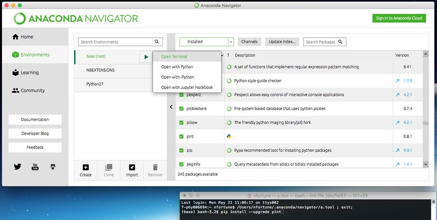
                                                                                                                                                                            1.2.2   Jupyter Notebooks
                                                                                                                                                                            The examples provided in this guide run Python within user friendly but somewhat oddly named
                                                                                                                                                                            Jupyter notebooks mentioned above. In some ways they look and act like Mathematica® notebooks, in-
                                                                                                                                                                            cluding the use of ‘cells’ (paragraphs of text, equations, or code) and the use of the shift+enter keys to
                                                                                                                                                                            execute the code in a cell. Jupyter notebooks are a spin-off of what is known as interactive Python (iPython)
                                                                                                                                                                            and in older examples on the web, you will still encounter references to iPython Notebook instead of Jupyter.
                                                                                                                                                                            This is also why Jupyter is spelled with a ‘py’ and why Jupyter notebook filenames still end with .ipynb.

                                                                                                                                                                            If the Jupyter notebook (formerly iPython notebook) interface is new to you, take time now to try the on-
                                                                                                                                                                            line interactive tutorial on how to run Python inside Jupyter notebooks. Go ahead, we’ll wait. The most
                                                                                                                                                                            important web pages in that tutorial are the first two: Notebook Basics andiPython: beyond plain Python.
                                                                                                                                                                            Once you are ready to learn how to add your own text and equations to Jupyter notebooks, see the third
                                                                                                                                                                            page (on Markdown Cells).

                                                                                                                                                                            Note that Jupyter notebooks are not the only way to write and run Python code. A bare-bones command
                                                                                                                                                                            line editor called IDLE is used by many beginning computer science students (and in the text Computational
                                                                                                                                                                            Physics) and a MATLAB® style interface called Spyder (again with the ‘py’ !) is used by many advanced
                                                                                                                                                                            Python programmers. The Python programs provided here will run in any of these environments. But this
                                                                                                                                                                            also means you can run Python programs encountered elsewhere within Jupyter notebooks!

                                                                                                                                                                            Within the Physics Department here at Smith College, we use the Jupyter notebook interface for two
                                                                                                                                                                            primary reasons: (1) running Python within the notebook provides a reproducible, self-documenting method
                                                                                                                                                                            of analyzing collected data, and (2) the ability to add explanatory notes, tables, figures, and equations within
                                                                                                                                                                            Jupyter notebooks means we can also use them as electronic lab notebooks for courses.

                                                                                                                                                                            1.2.3   Try it out!

                                                                                                                                                                            On a webserver

                                                                                                                                                                                                                                   2
A Short Guide to Using Python For Data Analysis In Experimental Physics
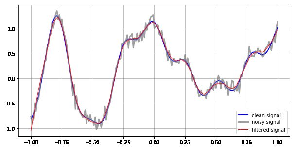
Jupyter notebooks are viewed and run using a web browser such as Firefox (just like this article in Authorea).
                                                                                                                                                                            That means they can also be run on a webserver that you access from a web browser and, as a result, it
                                                                                                                                                                            isn’t necessary to have Python installed on your own computer (provided you have internet access and all
                                                                                                                                                                            the Python packages you wish to use are already installed on the webserver).

                                                                                                                                                                            To try out the Python programs presented here using a Jupyter webserver hosted by Authorea, click
                                                                                                                                                                            the  Code button found to the left of many of the figures in this guide. This will reveal the .ipynb
                                                                                                                                                                            Jupyter notebook (and associated data files) containing the Python code used to generate that figure. Clicking
                                                                                                                                                                            on the notebook file name will launch the notebook in a new tab or window within your web browser . Clicking
                                                                                                                                                                            within a ‘cell’ (a block of text, equations, and or code, outlined by a rectangular border) and hitting SHIFT-
                                                                                                                                                                            ENTER will run any code in that cell and advance to the next one. Alternatively, you can make edits to the
                                                                                                                                                                            code in notebook (for example, adjust a smoothing parameter or change the name of a file) then select Run
                                                                                                                                                                            All from the Cell menu or Restart & Run All from the Kernel menu to rerun the program. For additional
                                                                                                                                                                            help, see the online interactive tutorial on how to run Python inside Jupyter notebooks.
Posted on Authorea 16 Jul 2021 — CC-BY 4.0 — https://doi.org/10.22541/au.152961025.52816543/v2 — This a preprint and has not been peer reviewed. Data may be preliminary.

                                                                                                                                                                            Many institutions host and configure their own Jupyter webservers suitable for Python programming. For
                                                                                                                                                                            example, Smith College physics students can upload and run any of the Jupyter notebooks included in this
                                                                                                                                                                            guide on the webserver https://jove.smith.edu, as this particular webserver has all the packages used
                                                                                                                                                                            here preinstalled. (Note to Smith students: contact the course instructor for an account).

                                                                                                                                                                            On your own computer
                                                                                                                                                                            The Authorea server will work for all of the examples except the (aptly named) Python packages Pint
                                                                                                                                                                            and Uncertainties used for numerical calculations using units and/or uncertainties, as those packages are not
                                                                                                                                                                            currently installed on that server (but maybe someday?). That said, you will want to write, run, and store
                                                                                                                                                                            your own data and programs on your own system. If you don’t have access to a local Jupyter webserver
                                                                                                                                                                            with the packages you need, you will want to install and run Python and Jupyter on your own computer.
                                                                                                                                                                            The good news is that everything needed is available for free (except the computer)! See Section 9: Installing
                                                                                                                                                                            Python for instructions on how to do this.

                                                                                                                                                                            2     Importing and exporting data

                                                                                                                                                                            There are many ways to import, export, and represent data in files. Here we provide just enough to get you
                                                                                                                                                                            started but it might very well be all you need. In these examples, we assume you have first entered the data
                                                                                                                                                                            into a spreadsheet program, then exported that data in ‘CSV’ (comma separated variable) file format. We
                                                                                                                                                                            use the CSV file format here because it is ubiquitous: all spreadsheets have the ability to export and import
                                                                                                                                                                            data in the CSV file format. Data in other common plain text file formats (such as tab delimited) can also
                                                                                                                                                                            be imported by making a few small modifications to the examples provided below.

                                                                                                                                                                            2.1    CSV spreadsheet file format

                                                                                                                                                                            Let’s look at a particular CSV data file titled Calibration 650nm.csv . The file consists of a single header
                                                                                                                                                                            row of text which we need to skip over when loading the numerical data, followed by three columns of data,
                                                                                                                                                                            one for each measured variable.

                                                                                                                                                                                                                                  3
A Short Guide to Using Python For Data Analysis In Experimental Physics
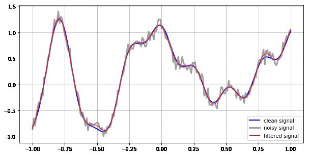
Here’s what the data looks like in spreadsheet form (grid lines not shown):

                                                                                                                                                                                                                   angle      V pd      V pd error
                                                                                                                                                                                                                 0.0e+00    3.24e+01     2.49e-02
                                                                                                                                                                                                                 1.5e+01    3.01e+01     1.54e-01
                                                                                                                                                                                                                 3.0e+01     2.4e+01     2.53e-01
                                                                                                                                                                                                                 4.5e+01    1.59e+01     2.85e-01
                                                                                                                                                                                                                 6.0e+01    7.78e+00     2.41e-01
                                                                                                                                                                                                                 7.5e+01    1.96e+00     1.33e-01
                                                                                                                                                                                                                 9.0e+01    3.57e-02     1.64e-02
                                                                                                                                                                                                                 1.05e+02   2.58e+00     1.53e-01
                                                                                                                                                                                                                 1.2e+02    8.95e+00     2.52e-01
                                                                                                                                                                                                                 1.35e+02   1.74e+01     2.85e-01
                                                                                                                                                                                                                 1.5e+02    2.56e+01     2.41e-01
                                                                                                                                                                                                                 1.65e+02   3.13e+01     1.34e-01
Posted on Authorea 16 Jul 2021 — CC-BY 4.0 — https://doi.org/10.22541/au.152961025.52816543/v2 — This a preprint and has not been peer reviewed. Data may be preliminary.

                                                                                                                                                                                                                 1.8e+02     3.3e+01     2.49e-02
                                                                                                                                                                                                                 1.95e+02   3.03e+01     1.54e-01
                                                                                                                                                                                                                 2.1e+02    2.39e+01     2.53e-01
                                                                                                                                                                                                                 2.25e+02   1.56e+01     2.85e-01
                                                                                                                                                                                                                 2.4e+02    7.55e+00     2.41e-01
                                                                                                                                                                                                                 2.55e+02   1.88e+00     1.33e-01
                                                                                                                                                                                                                 2.7e+02    3.38e-02     1.64e-02
                                                                                                                                                                                                                 2.85e+02   2.46e+00     1.53e-01
                                                                                                                                                                                                                 3.0e+02    8.51e+00     2.52e-01
                                                                                                                                                                                                                 3.15e+02   1.66e+01     2.85e-01
                                                                                                                                                                                                                 3.3e+02    2.47e+01     2.41e-01
                                                                                                                                                                                                                 3.45e+02   3.05e+01     1.34e-01
                                                                                                                                                                                                                 3.6e+02    3.25e+01     2.49e-02

                                                                                                                                                                                                                    Table 1: This is a caption

                                                                                                                                                                            Here’s what the first few lines of the same CSV spreadsheet file looks like when opened in a text editor
                                                                                                                                                                            (notice the commas separating the values within each row):

                                                                                                                                                                                  angle, V pd, V pd error
                                                                                                                                                                                  0.000000000000000000e+00,3.236249999999999716e+01,2.492398249033692462e-02
                                                                                                                                                                                  1.500000000000000000e+01,3.008079999999999998e+01,1.536232648449061544e-01
                                                                                                                                                                                  3.000000000000000000e+01,2.402850000000000108e+01,2.527732747539992997e-01

                                                                                                                                                                            2.2    loading data from a CSV file

                                                                                                                                                                            We are now going to use the Numerical Python (numpy) command loadtxt to load data from this CSV
                                                                                                                                                                            text file. Each column of data will become a Numerical Python (numpy) array.

                                                                                                                                                                            The process consists of two steps:

                                                                                                                                                                                                                                 4
1. importing the loadtxt command from Numerical Python
                                                                                                                                                                              2. using the loadtxt command to transfer the data from the file

                                                                                                                                                                            2.2.1   importing commands

                                                                                                                                                                            loadtxt is not part of the core Python language but is instead part of the Numerical Python package
                                                                                                                                                                            (numpy). We must therefore “import” it into our program before using. There are two common methods of
                                                                                                                                                                            doing this.

                                                                                                                                                                            In the first method, each individual function or module (such as loadtxt from numpy) is imported as needed
                                                                                                                                                                            . We call this the direct numpy import style.
                                                                                                                                                                            “‘ # example: direct import method
                                                                                                                                                                            from numpy import loadtxt #import just the numpy command loadtxt #from numpy import * #an alter-
Posted on Authorea 16 Jul 2021 — CC-BY 4.0 — https://doi.org/10.22541/au.152961025.52816543/v2 — This a preprint and has not been peer reviewed. Data may be preliminary.

                                                                                                                                                                            native method that imports all numpy commands. Be careful!
                                                                                                                                                                            This method is used, for example, in the excellent Python-based textbook Computational Physics by Mark
                                                                                                                                                                            Newman (Newman, 2013).

                                                                                                                                                                            Here is another example:

                                                                                                                                                                            #example: direct import method
                                                                                                                                                                            from numpy import sin, cos, array, pi               # import a few needed functions from the numpy package

                                                                                                                                                                            angle_in_degrees = array([0, 30, 60, 90]) # create an array with elements corresponding to 0, 30, 60, an
                                                                                                                                                                            angle_in_radians = angle_in_degrees * pi / 180     # convert to radians
                                                                                                                                                                            x = cos(angle_in_radians)                 # calculate cosine for each element in array, assign values to
                                                                                                                                                                            y = sin(angle_in_radians)                 # calculate sine for each element in array, assign values to a

                                                                                                                                                                            print(y)
                                                                                                                                                                            with result
                                                                                                                                                                            [0. 0.5 0.8660254       1.]

                                                                                                                                                                            In the second method, we first import all of the numpy package ( and, optionally, provide an abbreviation
                                                                                                                                                                            for numpy such as np.) We then add numpy. (or the abbreviation np.) as a prefix when using a function
                                                                                                                                                                            from the numpy package. We call this the traditional import style.
                                                                                                                                                                            # example: traditional import method

                                                                                                                                                                            import numpy as np # if you include ’as np’, ’numpy’ is replaced with the abbreviation ’np’
                                                                                                                                                                            We call this the traditional method because this is what you will find in the examples included in the official
                                                                                                                                                                            numpy user guide and quickstart tutorials.

                                                                                                                                                                                                                                  5
The key to using the traditional method is to be sure to specify that you are using a function or module from
                                                                                                                                                                            the numpy package by preceding it either with numpy or the abbreviation of your choice (such as np). This
                                                                                                                                                                            is why the loadtxt commands used in the examples below are written np.loadtxt instead of loadtxt.

                                                                                                                                                                            Here is another example:

                                                                                                                                                                            #example: traditional import method

                                                                                                                                                                            import numpy as np                                       # you only need to type this once in each program

                                                                                                                                                                            angle_in_degrees = np. array([0, 30, 60, 90]) # create an array with elements corresponding to 0, 30, 60
                                                                                                                                                                            angle_in_radians = angle_in_degrees * np.pi / 180      # convert to radians
                                                                                                                                                                            x = np.cos(angle_in_radians)                  # calculate cosine for each element in array, assign value
                                                                                                                                                                            y = np.sin(angle_in_radians)                 # calculate sine for each element in array, assign values t

                                                                                                                                                                            print(y)
Posted on Authorea 16 Jul 2021 — CC-BY 4.0 — https://doi.org/10.22541/au.152961025.52816543/v2 — This a preprint and has not been peer reviewed. Data may be preliminary.

                                                                                                                                                                            with the same result as before:

                                                                                                                                                                            [0. 0.5 0.8660254 1.]
                                                                                                                                                                            One one hand, the direct import method has the advantage of being lean, clean, and easy to read. Computer
                                                                                                                                                                            scientists love it. On the other hand, it does not work well if we need to use multiple packages containing
                                                                                                                                                                            identically named functions. For example, the math package math, the complex mathematics package cmath,
                                                                                                                                                                            the numerical python package numpy, and the numerical calculation of uncertainties package uncertainties
                                                                                                                                                                            all have trigonometric functions called sin and cos. To keep clear which function we are using from which
                                                                                                                                                                            package, and when, we will usually use the traditional import style for packages.

                                                                                                                                                                            2.2.2   importing the data file
                                                                                                                                                                            We now show how to use loadtxtto import the csv format spreadsheet file Calibration 650nm.csv. Unless
                                                                                                                                                                            specified otherwise, the data file is assumed to be in the same file folder as the Python program.

                                                                                                                                                                            The loadtxt command:

                                                                                                                                                                            # example: traditional import method

                                                                                                                                                                            import numpy as np # only need this once per program

                                                                                                                                                                            file_name = ’Calibration_650nm.csv’                         # replace with the name of your csv data file

                                                                                                                                                                            file_folder = ’’                                            # use this if your data file is in the same folder as

                                                                                                                                                                            #file_folder = ’/Users/nfortune/data’                       #   use this if data file is in a folder called ’data’
                                                                                                                                                                                                                                        #   inside the folder ’nfortune’ within the ’Users’ dire
                                                                                                                                                                                                                                        #   such as when using the Jupyter webserver jove.smith.
                                                                                                                                                                                                                                        #   this is called ’absolute addressing’

                                                                                                                                                                            #file_folder = ’data_subfolder/’                            # you can use this if data file is in a _subfolder_ ca

                                                                                                                                                                                                                                 6
# this is called ’relative addressing’
                                                                                                                                                                            data_file = file_folder + file_name

                                                                                                                                                                            angle, V_pd, V_pd_error        = np.loadtxt(data_file, delimiter = ’,’, skiprows = 1, usecols = (0, 1, 2), unp
                                                                                                                                                                            What these commands do:

                                                                                                                                                                            data file = file folder + file name tells Python what the name of the file is and where to find it! Tip:
                                                                                                                                                                            If you have trouble determining how to specify the file folder location for your data, an easy workaround is to
                                                                                                                                                                            first put the data in the same folder as your Python program, then either (a) set file folder = '' as in the
                                                                                                                                                                            example above or (b) replace np.loadtxt(file folder + file name, ...) with np.loadtxt(file name,
                                                                                                                                                                            ...) .

                                                                                                                                                                            delimiter = ',' tells loadtxt that your data is in comma separated variable format (CSV). The character
                                                                                                                                                                            used to separate one column of data from another is called the ‘delimiter.’ See the numpy.loadtxt manual
                                                                                                                                                                            page for details.
Posted on Authorea 16 Jul 2021 — CC-BY 4.0 — https://doi.org/10.22541/au.152961025.52816543/v2 — This a preprint and has not been peer reviewed. Data may be preliminary.

                                                                                                                                                                            skiprows = 1 tells loadtxt to skip over one row of text in the CSV file before looking for data to load into
                                                                                                                                                                            arrays. This is because the first row of text contains names for each column of data instead of data values
                                                                                                                                                                            (as shown in Table 1).

                                                                                                                                                                            unpack = True tells loadtxt that the data is in a ‘packed’ data format (in which each variable corresponds
                                                                                                                                                                            to a different column instead of to a different row )and therefore needs to be ‘unpacked’ when loaded. This
                                                                                                                                                                            is the typical arrangement for data in spreadsheets. Use unpack = False if the data is in an ‘unpacked’
                                                                                                                                                                            data format (in which each variable corresponds to a different row instead of a different column ).

                                                                                                                                                                            usecols = (0, 1, 2) says the data you are looking for is in the first 3 columns, which are numbered 0, 1,
                                                                                                                                                                            and 2 (because Python always starts from zero when counting). In our case, since there are only 3 columns
                                                                                                                                                                            of data and we want to use all three, this command is unnecessary. You could leave it out and everything
                                                                                                                                                                            would work just fine for this particular data file. If, however, you wanted to load data from a file with
                                                                                                                                                                            many columns but only needed data from column number 0, column number 3, and column number 4, you
                                                                                                                                                                            would need to include usecols = (0,3,4) within the loadtxt command.

                                                                                                                                                                            angle, V pd, V pd error = np.loadtxt(...) tells Numerical Python to create an array called angle
                                                                                                                                                                            and fill it with values from the first column of data in the CSV spreadsheet file, then create an array
                                                                                                                                                                            called V pd and fill it with values from the second column of data, and finally create an array called V pd -
                                                                                                                                                                            error and fill it with values from the third column of data. The result is three shiny new numpy data arrays
                                                                                                                                                                            we can use in our calculations.

                                                                                                                                                                            What if your data is in a different text file format (such as tab delimited)? In that case you can still use
                                                                                                                                                                            loadtxt to import your data as long as you modify the delimitercommand to match the file format. See
                                                                                                                                                                            the numpy.loadtxt manual page for details.

                                                                                                                                                                            2.3    saving data to a CSV file

                                                                                                                                                                                                                                  7
For completeness, we now provide an example of how to use the savetxt command from numpy to save data
                                                                                                                                                                            in csv format. There are many ways to save files in spreadsheet format but this is the simplest method we’ve
                                                                                                                                                                            found so far using numpy.

                                                                                                                                                                            Direct numpy import style:
                                                                                                                                                                            from numpy import savetxt, array                            #assumes you haven’t already imported these commands

                                                                                                                                                                            output_filename = ’output.csv’                              #provide a name for the new file
                                                                                                                                                                            header_row_text = ’angle, V_pd, V_pd_error’                 #make first row of file be a list of column names. Opti
                                                                                                                                                                            comment_text = ’’                                           #do not start header row with a ’#’. Optional.
                                                                                                                                                                            #comment_text = ’#’                                         #start the header row with a ’#’ . Default setting.

                                                                                                                                                                            data = array([angle, V_pd, V_pd_error]).T        #create a 2D matrix and transpose rows and columns (cle
                                                                                                                                                                            savetxt(output_filename, data, delimiter = ’,’, header = header_row_text, comments = comment_text)
                                                                                                                                                                            Traditional numpy import style:
                                                                                                                                                                            import numpy as np                                          #don’t import numpy again if already done once before
Posted on Authorea 16 Jul 2021 — CC-BY 4.0 — https://doi.org/10.22541/au.152961025.52816543/v2 — This a preprint and has not been peer reviewed. Data may be preliminary.

                                                                                                                                                                            output_filename = ’output.csv’                              #provide a name for the new file
                                                                                                                                                                            header_row_text = ’angle, V_pd, V_pd_error’                 #make first row of file be a list of column names. Opti
                                                                                                                                                                            comment_text = ’’                                           #do not start header row with a ’#’. Optional.
                                                                                                                                                                            #comment_text = ’#’                                         #start the header row with a ’#’ . Default setting.

                                                                                                                                                                            data = np.array([angle, V_pd, V_pd_error]).T     #create a 2D matrix and transpose rows and columns (cle
                                                                                                                                                                            np.savetxt(output_filename, data, delimiter = ’,’, header = header_row_text, comments = comment_text)
                                                                                                                                                                            Why do we need the line data = array([angle, V pd]).T ? We need it because ordinarily savetxt
                                                                                                                                                                            would save the data in what Python calls ‘unpacked’ format, a format in which each variable corresponds
                                                                                                                                                                            to a different row instead of to a different column. This is often convenient but is not what we wanted in
                                                                                                                                                                            this particular case. We therefore did the following clever trick before saving the data to a file: we created
                                                                                                                                                                            a 2D matrix of our data with the numpy command array([angle, V pd]), then used the .T command to
                                                                                                                                                                            transpose the matrix , thereby flipping the rows and columns.

                                                                                                                                                                            2.4    Other file handling methods
                                                                                                                                                                            For more advanced data handling of spreadsheet data files, large data sets, and/or the handling of binary data,
                                                                                                                                                                            you may wish to try the commands provided by the very popular Python Data Analysis Library package
                                                                                                                                                                            pandas or the big data Hierarchical Data Format (HDF5) using the Python interface package h5py (instead
                                                                                                                                                                            of those provided by numpy).

                                                                                                                                                                            3     Plotting data using error bars
                                                                                                                                                                            The most commonly used plotting package in Python is Matplotlib. Here’s an example of how to use it
                                                                                                                                                                            to generate plots with error bars representing the uncertainty in each data point. We use angle from the
                                                                                                                                                                            file 650 nm calibration.csv for the x-axis values, we use V pd for the y-axis values, and we use V pd delta
                                                                                                                                                                            for the uncertainty in the y-axis values.

                                                                                                                                                                                                                                  8
%matplotlib inline

                                                                                                                                                                            import matplotlib as mpl
                                                                                                                                                                            from matplotlib import pyplot as plt #this is the traditional method

                                                                                                                                                                            mpl.rc(’xtick’, labelsize = 18)             #use 18 point font for numbering on x axis
                                                                                                                                                                            mpl.rc(’ytick’, labelsize = 18)             #use 18 point font for numbering on y axis

                                                                                                                                                                            plt.figure(figsize = (7,5))                 #specify figure size as 7 x 5 inches
                                                                                                                                                                                                                        #for default size, type plt.figure()

                                                                                                                                                                            plt.xlabel(r"$\theta$ [degrees]", fontsize = 18) #label axis (using LaTeX commands)
                                                                                                                                                                            plt.ylabel(r"$V_{pd}$ [volts]", fontsize = 18)   #use 18 point font for label text

                                                                                                                                                                            plt.errorbar(angle, V_pd,
                                                                                                                                                                                xerr=None, yerr=V_pd_error,
                                                                                                                                                                                linestyle = ’none’,
                                                                                                                                                                                color = ’blue’,
Posted on Authorea 16 Jul 2021 — CC-BY 4.0 — https://doi.org/10.22541/au.152961025.52816543/v2 — This a preprint and has not been peer reviewed. Data may be preliminary.

                                                                                                                                                                                capsize = 3, capthick = 1)

                                                                                                                                                                            plt.show()
                                                                                                                                                                            The result is shown in Fig.1 below.

                                                                                                                                                                            What these commands do:

                                                                                                                                                                                 %matplotlib inline is an interactive Python (iPython) ’magic command’ used when running
                                                                                                                                                                                 Python within a Jupyter notebook. It allows the display of data plots within the notebook.

                                                                                                                                                                                 Tip: When running Jupyter notebooks within Authorea , the%matplotlib inline command
                                                                                                                                                                                 must precede the from matplotlib import pyplot command.

                                                                                                                                                                                 plt.figure() signifies the beginning of the plotting instructions specific to that figure.

                                                                                                                                                                                 plt.errorbar(angle, V pd, xerr = None, yerr=V pd delta) is the command that instructs
                                                                                                                                                                                 matplotlib to generate a x-y plot with error bars (as opposed to a bar graph or scatter plot, for
                                                                                                                                                                                 example). All four parameters (x, y, xerr, yerr) are required.

                                                                                                                                                                                 linestyle and color are used to customize the appearance of the data points. Linestyle =
                                                                                                                                                                                 None means there are no connecting lines between points. Color means the color of the error
                                                                                                                                                                                 bar lines and caps. The standard colors are blue, green, red, cyan, magenta, yellow, black, and
                                                                                                                                                                                 white (with corresponding abbreviations ‘b’, ‘g’, ‘r’, ‘c’, ‘m’, ‘y’, ‘k’, and ‘w’).

                                                                                                                                                                                 capsize, and capthick are used to customize the appearance of the error bars.       capsize =3
                                                                                                                                                                                 sets the width of the error bars to ‘3’ (in typesetter points), and capthick=1sets the thickness
                                                                                                                                                                                 of the drawn bars to ‘1’ (again in typesetter points). Note that if the capsize and capthick
                                                                                                                                                                                 commands are omitted, matplotlib will draw lines indicating the given uncertainty but will omit
                                                                                                                                                                                 the bars!

                                                                                                                                                                                                                                 9
plt.show() signifies the end of the plotting instructions and causes matplotlib to plot the data.

                                                                                                                                                                            For additional examples and information about other commands and options (including grid lines, tick
                                                                                                                                                                            marks, semilog plots, and log-log plots), please click on the links supplied here or search the online mat-
                                                                                                                                                                            plotlib.pyplot documentation.
Posted on Authorea 16 Jul 2021 — CC-BY 4.0 — https://doi.org/10.22541/au.152961025.52816543/v2 — This a preprint and has not been peer reviewed. Data may be preliminary.

                                                                                                                                                                            Figure 1: Photodiode voltage as a function of relative polarizer angle for light at 650 nm passing through
                                                                                                                                                                            two polarizers. Vpd corresponds to the voltage measured across a resistor placed in series with a photodiode
                                                                                                                                                                            and is linearly proportional to light intensity under these conditions. A change in polarization angle of the
                                                                                                                                                                            light (due to the Faraday effect, for example) can be detected as a change in photodiode voltage but the size
                                                                                                                                                                            of the change in voltage for a given change in polarization angle depends on the relative orientation of the
                                                                                                                                                                            two polarizers.

                                                                                                                                                                            4     Curve fitting

                                                                                                                                                                            4.1    mathematical modeling

                                                                                                                                                                             Curve fitting requires a mathematical model, initial estimates for the adjustable parameters in the model,
                                                                                                                                                                            and estimates of the uncertainty in the values of each data point. Here, we construct a mathematical model
                                                                                                                                                                            based on ”Malus’s Law” to describe light passing through two linear polarizers, as measured by a powered
                                                                                                                                                                            photodiode:

                                                                                                                                                                                                                                      1
                                                                                                                                                                                                     I(θ) = I0 cos2 (θ − θ0 ) + C =     I0 [1 + cos(2(θ − θ0 ))] + C                  (1)
                                                                                                                                                                                                                                      2

                                                                                                                                                                                                                                 10
where θ0 is the (fixed) angle of the first (reference) linear polarizer, θ is the (variable) angle of the second
                                                                                                                                                                            linear polarizer, θ − θ0 is the relative angle between them, and I0 is the maximum intensity of the light
                                                                                                                                                                            passing through both polarizers ( which occurs when θ = θ0 ). The offset C represents any ‘dc’ offset in the
                                                                                                                                                                            signal from the photo-detector (resulting in a nonzero signal in the absence of light), any additional light
                                                                                                                                                                            reaching the photo-detector that didn’t pass through the polarizers, and if the polarizers are not perfect
                                                                                                                                                                            (ideal), the fraction of light passing through but not polarized by both polarizers.

                                                                                                                                                                            Rewriting in terms of the measured output photodiode voltage Vpd , the relative polarizer angle φ = θ − θ0
                                                                                                                                                                            , and assuming a linear response between the photo-detector output voltage and light intensity, we have

                                                                                                                                                                                                                                                         1
                                                                                                                                                                                                              Vpd (φ) = V0 cos2 (φ) + V1 =                 V0 [1 + cos(2φ)] + V1                          (2)
                                                                                                                                                                                                                                                         2

                                                                                                                                                                            If, in addition, the variables V0 ,V1 , θ and θ0 and φ are independent of each other (which will be the case for
                                                                                                                                                                            ideal polarizers), then to first order, the uncertainty δVpd is given by (Hughes and Hase, 2010)
Posted on Authorea 16 Jul 2021 — CC-BY 4.0 — https://doi.org/10.22541/au.152961025.52816543/v2 — This a preprint and has not been peer reviewed. Data may be preliminary.

                                                                                                                                                                                                                s          2                               2                          2
                                                                                                                                                                                                                     ∂Vpd                              ∂Vpd                        ∂Vpd
                                                                                                                                                                                                    (δVpd ) =                    (δV0     )2   +                   (δφ)2   +                    (δV1 )2   (3)
                                                                                                                                                                                                                     ∂V0                                ∂φ                         ∂V1
                                                                                                                                                                                         q
                                                                                                                                                                                                2         2
                                                                                                                                                                            where δφ =       (δθ) + (δθ0 ) and which we will approximate as δθ as we are holding θ0 constant.

                                                                                                                                                                            Evaluating the partial derivatives in Eq. 3,
                                                                                                                                                                                                                s                        2                                                        2
                                                                                                                                                                                                                            4       δV0                                    2                   δV1
                                                                                                                                                                                                    δVpd = V0       (cos φ)                    + (−2 cos φ sin φ)              (δφ)2   +                  (4)
                                                                                                                                                                                                                                    V0                                                         V0

                                                                                                                                                                            The corresponding Python functions are
                                                                                                                                                                            # import numpy as np

                                                                                                                                                                            def polarization_model( phi_array, V_0, phi_0, V_1):
                                                                                                                                                                                return V_0 * (1 + np.cos(2 * (phi_array - phi_0)))/2 + V_1
                                                                                                                                                                            and
                                                                                                                                                                            # import numpy as np

                                                                                                                                                                            def photodiode_error(phi_array, delta_V_0, delta_phi, delta_V_1, V_0, phi_0):
                                                                                                                                                                                V_0_error= (delta_V_0 / V_0) * (np.cos(phi_array - phi_0))**2
                                                                                                                                                                                phi_error = (delta_phi) * (2 * np.cos(phi_array- phi_0) * np.sin(phi_array - phi_0))
                                                                                                                                                                                V_1_error= (delta_V_1 / V_0)
                                                                                                                                                                                fractional_error = np.sqrt(V_0_error **2 + phi_error **2 + V_1_error **2)
                                                                                                                                                                                return fractional_error * V_0

                                                                                                                                                                            We can determine δV1 and δV0 experimentally by measuring the statistical spread in the minimum and
                                                                                                                                                                            maximum values of Vpd (when φ = π2 radians and φ = 0, respectively). The polarizer angle θ is mechanically

                                                                                                                                                                                                                                                   11
set, so the uncertainty δφ depends on the accuracy of a nominally 15° step change in angle θ with the
                                                                                                                                                                            apparatus at hand.

                                                                                                                                                                            Now we encounter an apparent conundrum: we want to use the curve fit to determine a best estimate for V0
                                                                                                                                                                            but solving for δV requires us to already have a numerical value for V0 . How do we determine the numerical
                                                                                                                                                                            values for δVpd (θ) needed to find a best estimate of V0 if we don’t already know V0 ? This, however, is not
                                                                                                                                                                            the impasse that it might seem. The curve fitting algorithm already requires that we supply an initial guess
                                                                                                                                                                            for the parameters. In this situation, then, we can carry out the curve fitting algorithm a second or third
                                                                                                                                                                            time instead of just once, each time using the best fit values output by the algorithm in the previous fit as
                                                                                                                                                                            our new initial values for the new fit. Once the output values match the input values (within uncertainty),
                                                                                                                                                                            we stop. When the output values match the input values, we say the results are self-consistent.

                                                                                                                                                                            Here is the procedure for finding self-consistent ‘best fit’ values from curve-fitting:
                                                                                                                                                                              1. Make a rough initial guess for the parameters V0 , V1 , and θ0 from a graph of the data.
                                                                                                                                                                              2. Use the values of V0 , V1 , and θ0 output by the curve-fitting routine as a new ‘initial guess’
                                                                                                                                                                              3. Repeat the curve fit (using each output as a new input) until V0 stops changing.
Posted on Authorea 16 Jul 2021 — CC-BY 4.0 — https://doi.org/10.22541/au.152961025.52816543/v2 — This a preprint and has not been peer reviewed. Data may be preliminary.

                                                                                                                                                                            Note: if you know how to do programming in Python, this would be a great place to simplify your life by
                                                                                                                                                                            introducing a while loop into the code that repeats the curve fit until the results become self-consistent.
                                                                                                                                                                            We plan to add a section illustrating how to do that in a future version of this guide.

                                                                                                                                                                            4.2     fitting the model to data
                                                                                                                                                                            4.2.1   calculating best fit values

                                                                                                                                                                            We now turn to the actual Python code for non-linear curve fitting. Notice that this is a “weighted” fit,
                                                                                                                                                                            in that the stated uncertainty of each data point is taken into account during the fit. Practically speaking,
                                                                                                                                                                            this means the curve-fitting routine tries harder to match the model to the data at points with a smaller
                                                                                                                                                                            uncertainty (although it may not succeed) because those points are given greater importance (’weight’). This
                                                                                                                                                                            is as it should be, and is also needed to calculate a numerically accurate chi-square value for a determination
                                                                                                                                                                            of the “goodness of fit.”

                                                                                                                                                                            Here we assume that values have already been experimentally determined for uncertainties in V0 , V1 , and θ.
                                                                                                                                                                            We will therefore leave these unchanged throughout the curve-fitting process.
                                                                                                                                                                            # measured uncertainties
                                                                                                                                                                            delta_V0 = 0.020           # mV, after averaging
                                                                                                                                                                            delta_V1 = 0.014           # mV, after averaging
                                                                                                                                                                            delta_theta = 0.5 * np.pi / 180 # 0.5 degrees, in radians
                                                                                                                                                                            Now let’s take care of the initial setup:
                                                                                                                                                                            # initial guess for polarization models
                                                                                                                                                                            V0 = 30.0    #initial guess, in mV
                                                                                                                                                                            V1 = 0.02    #initial guess, in mV

                                                                                                                                                                            theta = angle * np.pi / 180            # convert from degrees to radians

                                                                                                                                                                            theta0 = -2.0 * np.pi / 180          #initial guess for offset angle of 2 degree, in radians

                                                                                                                                                                                                                                  12
initial_guess = np.array([V0, theta0, V1])
                                                                                                                                                                            initial_error = np.array([delta_V0, delta_theta, delta_V1])
                                                                                                                                                                            old_fit = np.copy(initial_guess) # save a copy to compare new with old

                                                                                                                                                                            estimated_error = photodiode_error(theta, delta_V0, delta_theta, delta_V1,
                                                                                                                                                                                V0, theta0)    #propagate uncertainty using initial values
                                                                                                                                                                            Finally let’s run the curve fit command:
                                                                                                                                                                            # load curve_fit routine from scipy
                                                                                                                                                                            from scipy.optimize import curve_fit # import method used here

                                                                                                                                                                            # alternative method (as recommended in https://docs.scipy.org/doc/scipy/reference.api.html)
                                                                                                                                                                            #from scipy import optimize
                                                                                                                                                                            #fit, covariance = optimize.curve_fit(...)

                                                                                                                                                                            #run curve_fit for polarization_model
                                                                                                                                                                            fit, covariance = curve_fit(polarization_model, theta, V_pd,
                                                                                                                                                                                                        p0 = initial_guess,
Posted on Authorea 16 Jul 2021 — CC-BY 4.0 — https://doi.org/10.22541/au.152961025.52816543/v2 — This a preprint and has not been peer reviewed. Data may be preliminary.

                                                                                                                                                                                                        sigma = estimated_error, absolute_sigma = True)

                                                                                                                                                                            error = np.sqrt(np.diag(covariance))

                                                                                                                                                                            print(old_fit)
                                                                                                                                                                            print(fit)

                                                                                                                                                                            old_fit = np.copy(fit)

                                                                                                                                                                            print()
                                                                                                                                                                            print(’V_0    = ’,’{:.3f}’.format(fit[0]), ’±’, ’{:.3f}’.format(error[0]), ’ mV’)
                                                                                                                                                                            print(’V_1 = ’,’{:.4f}’.format(fit[2]), ’±’, ’{:.3f}’.format(error[2]), ’ mV’)
                                                                                                                                                                            print(’theta_0 = ’,’{:.4f}’.format(fit[1]), ’±’, ’{:.4f}’.format(error[1]), ’radian’)
                                                                                                                                                                            print(’       = ’,’{:.4f}’.format(fit[1]*180/np.pi), ’±’, ’{:.4f}’.format(error[1]*180/np.pi), ’degrees’
                                                                                                                                                                            Here are the results after the first iteration:
                                                                                                                                                                            V_0     =     32.631    ±   0.024 mV
                                                                                                                                                                            V_1     =      0.023    ±   0.016 mV
                                                                                                                                                                            theta_0 =     -0.0203   ±   0.0018 radian
                                                                                                                                                                                    =     -1.162    ±   0.102 degrees
                                                                                                                                                                            We now use the output values for V0 and V1 as the new input values and recalculate the estimated error for
                                                                                                                                                                            each Vpd (θ) value:
                                                                                                                                                                            new_initial_values = np.array([fit[0], fit[1], fit[2]])

                                                                                                                                                                            estimated_error = photodiode_error(theta, delta_V0, delta_theta, delta_V1,
                                                                                                                                                                                fit[0], fit[1]) # propagate error using new values for V0, etc

                                                                                                                                                                            fit, covariance = curve_fit(polarization_model, theta, V_pd,
                                                                                                                                                                                                        p0 = new_initial_values,
                                                                                                                                                                                                        sigma = estimated_error, absolute_sigma = True)

                                                                                                                                                                            error = np.sqrt(np.diag(covariance))

                                                                                                                                                                                                                               13
print(old_fit)
                                                                                                                                                                            print(fit)

                                                                                                                                                                            old_fit = np.copy(fit)

                                                                                                                                                                            V_pd_model = polarization_model(theta, fit[0], fit[1], fit[2])
                                                                                                                                                                            residual = V_pd - V_pd_model

                                                                                                                                                                            data_uncertainty = photodiode_error(theta, delta_V0, delta_theta, delta_V1, fit[0], fit[1])

                                                                                                                                                                            chisq = sum((residual/ data_uncertainty)**2) #typo corrected
                                                                                                                                                                            degrees_of_freedom = len(residual) - len(initial_guess)
                                                                                                                                                                            reduced_chisq = chisq / degrees_of_freedom # this should be close to one
                                                                                                                                                                            CDF = chi2.cdf(chisq, degrees_of_freedom)   # this should be close to 50 percent

                                                                                                                                                                            print(’chi-square         = ’,chisq)
                                                                                                                                                                            print(’degrees of freedom = ’,degrees_of_freedom)
Posted on Authorea 16 Jul 2021 — CC-BY 4.0 — https://doi.org/10.22541/au.152961025.52816543/v2 — This a preprint and has not been peer reviewed. Data may be preliminary.

                                                                                                                                                                            print(’reduced chi-square = ’,reduced_chisq)
                                                                                                                                                                            print(’fractional probability of chisq \selectlanguage{english}[?]’, chisq, ’for ’, degrees_of_freedom,
                                                                                                                                                                            and continue in this way until the value V 0 stops changing.

                                                                                                                                                                            4.2.2   graphing the results
                                                                                                                                                                            Our final numerical results are:
                                                                                                                                                                            V_0     =    32.629    +-   0.020 mV
                                                                                                                                                                            V_1     =     0.022    +-   0.013 mV
                                                                                                                                                                            theta_0 =    -0.0202   +-   0.0020 radian
                                                                                                                                                                                    =    -1.155    +-   0.112 degrees
                                                                                                                                                                            We can now graphically compare the original data with our model (Eq. 2 ) using the best fit values for the
                                                                                                                                                                            parameters:
                                                                                                                                                                            plt.figure(figsize = (11,8))                          #specify figure size as 7 x 5 inches
                                                                                                                                                                                                                                 #for default size, type plt.figure()

                                                                                                                                                                            plt.xlabel(r"$\theta$ [degrees]", fontsize = 18) #label axis (using LaTeX commands)
                                                                                                                                                                            plt.ylabel(r"$V_{pd}$ [volts]", fontsize = 18)   #use 18 point font for label text

                                                                                                                                                                            # plot the data as before in blue
                                                                                                                                                                            plt.errorbar(angle, V_pd,
                                                                                                                                                                                xerr=None, yerr=V_pd_error,
                                                                                                                                                                                linestyle = ’none’,
                                                                                                                                                                                color = ’blue’,
                                                                                                                                                                                capsize = 3, capthick = 1, label = "data")

                                                                                                                                                                            #create curve showing fit to data
                                                                                                                                                                            angle_fit = np.linspace(0, 360, 180)
                                                                                                                                                                            theta_fit = angle_fit * np.pi / 180
                                                                                                                                                                            V_pd_fit = polarization_model(theta_fit, fit[0], fit[1], fit[2])

                                                                                                                                                                            #plot the curve fit in red

                                                                                                                                                                                                                                14
plt.errorbar(angle_fit, V_pd_fit, xerr = None, yerr = None, color = ’red’, label = ’fit’ )
                                                                                                                                                                            plt.xlim(-15, 375)
                                                                                                                                                                            plt.ylim(-2.5, 40)
                                                                                                                                                                            plt.xticks([0,   30, 60, 90, 120, 150, 180, 210, 240, 270, 300, 330, 360],
                                                                                                                                                                                       (’0’, ’’, ’’, 90, ’’, ’’, 180, ’’, ’’, 270, ’’, ’’, 360))
                                                                                                                                                                            plt.legend(loc = ’best’)

                                                                                                                                                                            plt.show()
                                                                                                                                                                            The results are plotted in Fig. 2 below.
Posted on Authorea 16 Jul 2021 — CC-BY 4.0 — https://doi.org/10.22541/au.152961025.52816543/v2 — This a preprint and has not been peer reviewed. Data may be preliminary.

                                                                                                                                                                                  Figure 2: Curve fit of Eq. 2 to calibration data for 650 nm using best-fit values for parameters.

                                                                                                                                                                            At first glance, the model appears to describe the data quite well, with the possible exception of the points
                                                                                                                                                                            where Vpd (θ) is a maximum. To quantify the goodness of fit, however, we will need to evaluate the fit
                                                                                                                                                                            residuals and chi-square test goodness of fit. See section 4.3.

                                                                                                                                                                            Note: there are additional features of the curve fit function not demonstrated here, including the ability to
                                                                                                                                                                            set lower and upper bounds on each of the adjustable parameters. For example, setting the option bounds
                                                                                                                                                                            = ([0, -np.pi, -1.0], [np.inf, +np.pi, 1.0])
                                                                                                                                                                             would then force the best fit parameters to stay in the range 0 ≤ I0 , −π ≤ θ0 ≤ π in rad, and −1 ≤
                                                                                                                                                                            offset ≤ +1. See the scipy.optimize.curve fit documentation for details.

                                                                                                                                                                            4.3    Evaluating the goodness of fit

                                                                                                                                                                            We now have a best fit of the model to the data. How good a fit is it? That is, how well does the model
                                                                                                                                                                            describe the data, taking into account the uncertainty in each data point? Two quick ways to test the

                                                                                                                                                                                                                                 15
goodness of fit of the model to the data are through calculations of the residuals and the reduced chi-square
                                                                                                                                                                            value. See (Hughes and Hase, 2010) and (Berendsen, 2011).

                                                                                                                                                                            4.3.1   residuals

                                                                                                                                                                            The calculation of the residual errors is easy once the model is defined and the fitting parameters deter-
                                                                                                                                                                            mined. Here is an example:
                                                                                                                                                                            # theta = angle * np.pi / 180        # convert to radians

                                                                                                                                                                            V_pd_model = polarization_model_1(theta, fit[0], fit[1], fit[2])
                                                                                                                                                                            residual = V_pd - V_pd_model
                                                                                                                                                                            The corresponding plot is shown in Fig. 3 below.
Posted on Authorea 16 Jul 2021 — CC-BY 4.0 — https://doi.org/10.22541/au.152961025.52816543/v2 — This a preprint and has not been peer reviewed. Data may be preliminary.

                                                                                                                                                                            Figure 3: residual error compared with estimated measurement uncertainty for ±σ (in red) and ±2σ (in
                                                                                                                                                                            orange). Most points are within one or two standard deviations of zero residual error, as expected for a
                                                                                                                                                                            good fit to the data using Malus’s law, but the points do not appear randomly distributed. Instead, there
                                                                                                                                                                            is a weak angular dependence suggesting a small uncorrected systematic misalignment of the light source
                                                                                                                                                                            and/or polarizers with respect to the detector.

                                                                                                                                                                            The residuals are generally within one standard deviation of zero but do not appear randomly distributed.
                                                                                                                                                                            Instead there is a weak residual angular dependence. One possibility is that light beam, polarizers, and
                                                                                                                                                                            detector are not perfectly centered and the polarization is not completely uniform across the entire surface
                                                                                                                                                                            of the polarizer. Malus’s law does not however appear to be in question. Rather, the residuals indicate a
                                                                                                                                                                            small level of polarizer-angle dependent systematic error.

                                                                                                                                                                            4.3.2
                                                                                                                                                                            4.3.3   chi-square test

                                                                                                                                                                                                                                 16
Once the residuals have been calculated, the determination of the corresponding chi-square value for goodness
                                                                                                                                                                            of fit is straightforward. Here is an example:

                                                                                                                                                                            from scipy.stats import chi2                   # ’chi-square’ goodness of fit calculation

                                                                                                                                                                            chisq = sum((residual/ data_uncertainty)**2) # typo corrected 2/1/2019
                                                                                                                                                                            degrees_of_freedom = len(residual) - len(initial_guess)
                                                                                                                                                                            reduced_chisq = chisq / degrees_of_freedom # this should be close to one
                                                                                                                                                                            CDF = chi2.cdf(chisq, degrees_of_freedom)   # this should be close to 50 percent

                                                                                                                                                                            print(’chi-square         = ’,chisq)
                                                                                                                                                                            print(’degrees of freedom = ’,degrees_of_freedom)
                                                                                                                                                                            print(’reduced chi-square = ’,reduced_chisq)
                                                                                                                                                                            print(’fractional probability of chisq [?]’, chisq, ’for ’, degrees_of_freedom, ’dof is’, CDF)
                                                                                                                                                                            Ideally, if the model describes the data AND the estimated uncertainty of each point has been accurately
                                                                                                                                                                            determined, the reduced chi-square value would be approximately equal to one (for large ν) and the fractional
                                                                                                                                                                            probability of χ2 values larger and smaller than that measured would both be approximately 50%. Statis-
Posted on Authorea 16 Jul 2021 — CC-BY 4.0 — https://doi.org/10.22541/au.152961025.52816543/v2 — This a preprint and has not been peer reviewed. Data may be preliminary.

                                                                                                                                                                            tically, however, we expect some reasonable random variation from the expected mean value of ν for χ2min ,
                                                                                                                                                                            meaning that statisticians generally will not reject the “null hypothesis” (that the model describes the data
                                                                                                                                                                                                                                                                          2
                                                                                                                                                                            and all deviations can be reasonably attributed to expected random variation)  √ as long as χmin is within 2
                                                                                                                                                                                                                                      2
                                                                                                                                                                            standard deviations ( 2σ ) of the mean value. Here, χmean = ν and σν = 2ν (Hughes and Hase, 2010)
                                                                                                                                                                            , so the criterion can be reexpressed as

                                                                                                                                                                                                                        √                   √
                                                                                                                                                                                                                   ν − 2 2ν ≤ χ2 min ≤ ν + 2 2ν                                       (5)

                                                                                                                                                                            Here are the results for the fit shown in Fig. 2:

                                                                                                                                                                                  chi-square test value χ2min = 15.3
                                                                                                                                                                                  degrees of freedom ν = 25 - 3 = 22
                                                                                                                                                                                  reduced chi-square    = 0.694
                                                                                                                                                                                  fractional probability of χ2 [?] 15.3 is 15.0%
                                                                                                                                                                                  fractional probability of χ2 > 15.3 is 85.0%

                                                                                                                                                                                       √
                                                                                                                                                                            Here, σ = 2 ν = 6.6, χ2mean − σ = 15.4, and χ2mean + σ = 28.6, indicating that our result is very slightly
                                                                                                                                                                            outside one standard deviation of the mean but well within two standard deviations. We conclude that
                                                                                                                                                                            we have acceptably good agreement between model and experiment at this level of experimental precision
                                                                                                                                                                            but that further improvements in apparatus design, measurement method, and reduction in uncertainty are
                                                                                                                                                                            merited.

                                                                                                                                                                            5     Data Smoothing and Differentiation

                                                                                                                                                                            5.1    Savitzky-Golay filters

                                                                                                                                                                                                                                   17
Data smoothing is a way of reducing time varying noise in measured data so as to reveal the underlying
                                                                                                                                                                            dependence of the measured variable on a different variable (such as an applied voltage or an external
                                                                                                                                                                            magnetic field). In most cases, the computer is acting as a digital low pass filter. It differs from an analog
                                                                                                                                                                            low pass output filter in that the filtering is done by us using a computer after the measurement is complete
                                                                                                                                                                            rather than by the instrument itself. Like the signal averaging done by a digital oscilloscope — the point by
                                                                                                                                                                            point averaging of a periodic signal — data smoothing seeks to separate random noise from a reproducible
                                                                                                                                                                            signal, but here the measured ‘signal’ to be smoothed is not assumed to be periodic and is in fact usually a
                                                                                                                                                                            function of a variable other than time. An example would be the measurement of current as a function of
                                                                                                                                                                            applied voltage for a non-ohmic device.

                                                                                                                                                                            The SciPy (for scientific python) package offers an exhaustive list of signal processing functions useful for
                                                                                                                                                                            the digital filtering. If you have some programming experience in Python, you may wish to design your own
                                                                                                                                                                            filter, perhaps using the lower level scipy.signal filter design tools. There are, for example, a wide variety of
                                                                                                                                                                            spectral analysis and peak finding routines for frequency data that we will not explore further here.

                                                                                                                                                                            In this getting start guide, we will focus on the use of a particularly useful and easy to use ready-made filter
                                                                                                                                                                            for data smoothing of y (xi ) data equally spaced in x: the Savitzky-Golay low pass filter (Savitzky and
Posted on Authorea 16 Jul 2021 — CC-BY 4.0 — https://doi.org/10.22541/au.152961025.52816543/v2 — This a preprint and has not been peer reviewed. Data may be preliminary.

                                                                                                                                                                            Golay, 1964; Steinier et al., 1972). This filter works by fitting a subset of data points adjacent to a particular
                                                                                                                                                                            data point with a low-degree polynomial, evaluating the polynomial at that point, and then repeating the
                                                                                                                                                                            process for each data point. The set of points centered about a particular data point is called the ‘filter
                                                                                                                                                                            window’ and the number of points in the filter window is called the window length (although width would
                                                                                                                                                                            seem more apt). The picture here might be of a small window in a cabin looking out upon a nearby data
                                                                                                                                                                            stream. The window reveals a small subset of points at a time as the data “streams” by. The fit is carried
                                                                                                                                                                            out on the points seen through the window, and repeated for each point in the stream.

                                                                                                                                                                            As a bonus, the SciPy Savitzky-Golay filter function scipy.signal.savgol filter can also be used to
                                                                                                                                                                            numerically differentiate the smoothed data (again, provided the data is “equally spaced”). This is a
                                                                                                                                                                            particularly useful feature. For example, we might directly measure I (V ) for a particular non-ohmic device
                                                                                                                                                                                                                                                                           dI
                                                                                                                                                                            (such as a light bulb or LED) but be more interested theoretically in the differential current dV as a function
                                                                                                                                                                            of applied voltage V . Experimentally, the noise fluctuations in a measurement of I as a function of V might
                                                                                                                                                                                                              dI
                                                                                                                                                                            preclude a direct calculation of dV  . By first smoothing the data using a Savitzky-Golay filter to reduce the
                                                                                                                                                                                                                 dI
                                                                                                                                                                            noise, a meaningful calculation of dV   as a function of V can now be carried out.
                                                                                                                                                                            There are a few practical constraints:
                                                                                                                                                                              1. the window length must be an odd number
                                                                                                                                                                              2. the polynomial order (1, 2, 3, . . . ) must be less than the window length
                                                                                                                                                                              3. the data points are assumed to be “evenly spaced” (for example in time, voltage, or magnetic field)
                                                                                                                                                                            For example, when measuring current I as a function of applied voltage V from -10 to +30 V in equal steps
                                                                                                                                                                            of 0.1 volts, specifying a window length of 21 points and a second order polynomial fit would correspond
                                                                                                                                                                            to a fitting a quadratic function to a set of 21 points spanning a 2 V range centered about a particular
                                                                                                                                                                            data point (including that point), then repeating that process for each subsequent data point. In the SciPy
                                                                                                                                                                            implementation, this repeated fitting over a moving data stream is done automatically for us.

                                                                                                                                                                            As noted above, the number of points included in the subset and the order of the polynomial must be specified
                                                                                                                                                                            by the user. In all data smoothing routines, there is a tradeoff between the degree of smoothing and the
                                                                                                                                                                            ability to resolve small features in the underlying signal; data smoothing is not a substitute for working as
                                                                                                                                                                            carefully as possible to minimize the measurement noise and maximize the accuracy and precision of the
                                                                                                                                                                            originally measured data! In the end, the ‘best values’ for these parameters are usually determined by trial
                                                                                                                                                                            and error. Keep track of the values used when determining the resolution of your experiment!

                                                                                                                                                                                                                                   18
5.1.1   Scipy.Signal.Savgol filter

                                                                                                                                                                            This filter can be implemented in Python with just two lines of code: one to import from
                                                                                                                                                                            the scipy.signal module the function savgol filter, and one more to carry out the data smoothing.

                                                                                                                                                                            We first need to specify two parameters:

                                                                                                                                                                              1. window length, the number of adjacent data points we wish to include in the fit
                                                                                                                                                                              2. polyorder, the order of the polynomial fit (where 0 = constant, 1 = linear, 2 = quadratic, and 3 =
                                                                                                                                                                                 cubic)
                                                                                                                                                                            If we also want to calculate the slope of the data at each point by taking a derivative, we then need to specify
                                                                                                                                                                            two additional parameters :
Posted on Authorea 16 Jul 2021 — CC-BY 4.0 — https://doi.org/10.22541/au.152961025.52816543/v2 — This a preprint and has not been peer reviewed. Data may be preliminary.

                                                                                                                                                                              1. deriv, the order of the derivative (where 0 = no derivative, 1 = first derivative, 2 = 2nd derivative,. . . )
                                                                                                                                                                              2. delta, the spacing of the samples to which the filter will be applied.
                                                                                                                                                                                                                                      dI
                                                                                                                                                                            As an example, suppose we want again to determine dV         from a measurement of I (V ) for applied volt-
                                                                                                                                                                            ages between -10 V and +30 V and that measurements were made evenly spaced in voltage with a step size
                                                                                                                                                                            of 0.1 V. If so, we then specify that deriv = 1 and delta = 0.1 within the savgol filter function.

                                                                                                                                                                            Finally, for the computed derivative to be physically and quantitatively meaningful,

                                                                                                                                                                              1. the order of the polynomial fit needs to be greater than the order of derivative (!)
                                                                                                                                                                              2. The delta value needs to be correctly specified. If unspecified, it is assumed that delta = 1.
                                                                                                                                                                            As usual, there are additional optional settings, including options for how to handle data near the endpoints
                                                                                                                                                                            (see mode): the default (mode = interp) is to fit the last window length / 2 points to a polynomial of order
                                                                                                                                                                            polyorder. For this and other details, see the Scipy reference manual page.

                                                                                                                                                                            5.1.2   Sample Python code
                                                                                                                                                                            Here is an example of how to use the SciPy function savgol filter for data smoothing.
                                                                                                                                                                            from scipy.signal import savgol_filter

                                                                                                                                                                            window_width = 25           #   set number of points over which data is fit and smoothed equal to 25
                                                                                                                                                                                                        #   window_width must be an odd number
                                                                                                                                                                            polynomial_order = 2        #   set order of polynominal used to fit data equal to 2
                                                                                                                                                                                                        #   polynomial_order must be less than window_width

                                                                                                                                                                            data_spacing = 0.1          # data_spacing = x_1 - x_0 for data y(x_0), y(x_1), ....

                                                                                                                                                                            smoothed_data   = savgol_filter(noisy_data, window_width, polynomial_order) #smooth data
                                                                                                                                                                            data_derivative = savgol_filter(noisy_data, window_width, polynomial_order, deriv = 1, delta = 0.1) #tak
                                                                                                                                                                            An example of data smoothing using the Savitzky-Golay low pass filter is shown in Fig 4. Since for real
                                                                                                                                                                            experimental data the original ‘clean signal’ is unknown, the degree of smoothing is always a matter of

                                                                                                                                                                                                                                   19
judgement. A comparison of several different smoothing values (not shown) can be useful in discerning the
                                                                                                                                                                            best choice of parameters and the effective resolution of your processed data (and any derivatives) .
Posted on Authorea 16 Jul 2021 — CC-BY 4.0 — https://doi.org/10.22541/au.152961025.52816543/v2 — This a preprint and has not been peer reviewed. Data may be preliminary.

                                                                                                                                                                                  Figure 4: Use of a Savitzky-Golay low pass filter to smooth (artificially generated) noisy data.

                                                                                                                                                                            In general, increasing the window width increases the degree of smoothing, causing small features in the
                                                                                                                                                                            original ‘clean signal’ to disappear; decreasing the window width decreasing the degree of smoothing, causing
                                                                                                                                                                            artificial features (arising from the noise) to emerge. Increasing the order of the polynomial while holding the
                                                                                                                                                                            window width constant decreases the degree of noise reduction but is needed for if there is significant data
                                                                                                                                                                            curvature over the width of the smoothing window. To see this for yourself, this click first on the  Code
                                                                                                                                                                            button, then on the file name Smooth and differentiate.ipynb to open and view the underlying Jupyter
                                                                                                                                                                            notebook containing the Python code used to generate this figure. Once opened, you can vary the smoothing
                                                                                                                                                                            parameters and re-run the notebook to see the changes. You can also download the notebook to your own
                                                                                                                                                                            computer as a template.

                                                                                                                                                                            5.2     Butterworth filters

                                                                                                                                                                            Everyone has there own favorite low pass filter smoothing routine. The Savitky-Golay method presented
                                                                                                                                                                            here is a useful and intuitive place to start but it is not necessarily better or worse than any other smoothing
                                                                                                                                                                            routine. For more advanced filtering methods and examples, see the SciPy Cookbook and the SciPy signal
                                                                                                                                                                            processing reference guide.

                                                                                                                                                                            Two examples of particular interest from the SciPy Cookbook involve Butterworth filters,        which are
                                                                                                                                                                            designed to have as flat a frequency response as possible over the range of frequencies to be passed while
                                                                                                                                                                            still filtering out unwanted frequencies (such as high frequency noise):

                                                                                                                                                                              1. a Butterworth bandpass filter to filter out high frequency noise, low frequency noise, and dc drift
                                                                                                                                                                              2. a Butterworth low pass filter for general data smoothing

                                                                                                                                                                            Note: The use of a Butterworth filter requires the specification of a cutoff frequency (or frequencies). For a
                                                                                                                                                                            digital Butterworth filter, varying the value of the normalized Nyquist frequency between zero and one will
                                                                                                                                                                            change the degree of smoothing provided. Lower values produce greater smoothing of the data.

                                                                                                                                                                                                                                  20
The example in Fig. 5 below uses a 3rd order digital Butterworth low-pass filter with a Nyquist frequency of
                                                                                                                                                                            0.13 (see attached code) to smooth the same signal as in Fig. 4 ; the originalSciPy cookbook example uses a
                                                                                                                                                                            frequency of 0.05. See the SciPy cookbook and the Jupyter notebook attached to this figure for additional
                                                                                                                                                                            details.
Posted on Authorea 16 Jul 2021 — CC-BY 4.0 — https://doi.org/10.22541/au.152961025.52816543/v2 — This a preprint and has not been peer reviewed. Data may be preliminary.

                                                                                                                                                                            Figure 5: Use of a digital Butterworth low-pass filter (and some fancy footwork) to smooth the same data
                                                                                                                                                                            as in Fig. 4.

                                                                                                                                                                            5.3    Differentiation
                                                                                                                                                                            One of the most common reasons for data smoothing is to then be able to differentiate the data. As
                                                                                                                                                                            noted earlier in section 5.1.1, one of the advantages of using scipy.signal.savgol filter is that the data
                                                                                                                                                                            smoothing and differentiation can be done in a single step (when working with evenly spaced data). Here is
                                                                                                                                                                            an example (for the data originally shown in Fig. 4):

                                                                                                                                                                            Figure 6: Filtered signal and first derivative of data shown in FIg. 4 . Numerical results calculated (from
                                                                                                                                                                            noisy signal) using the SciPy Savitzky-Golay filter function (window width = 25, polyorder = 2).

                                                                                                                                                                                                                                21
More generally, however, the numerical derivative of a suitably filtered signal y (x) can also be evaluated
                                                                                                                                                                            at each x value using the numpy function gradient where for a 1D array of data the gradient will be the
                                                                                                                                                                                                   dy
                                                                                                                                                                            same as the derivative dx . According to the numpy.gradient reference page , this function “calculates the
                                                                                                                                                                            gradient using second order accurate central differences in the interior points and either first or second order
                                                                                                                                                                            accurate one-sides (forward or backwards) differences at the boundaries. ” It also has the advantage of not
                                                                                                                                                                            requiring equally spaced data values. See the reference page for further examples and details.

                                                                                                                                                                                                                                                          df
                                                                                                                                                                            Here is a simple example of how to use gradient to numerically calculate dx      from smoothed f (xi ) data
                                                                                                                                                                            without knowledge of the function f (x), assuming that the data is equally spaced with a sample distance dx
                                                                                                                                                                            of 0.1:

                                                                                                                                                                            import numpy as np

                                                                                                                                                                            data_derivative_array = np.gradient(smoothed_data_array, 0.1)
                                                                                                                                                                            Gradient can also used with unequally spaced values, if those values are provided. Here is one example:
Posted on Authorea 16 Jul 2021 — CC-BY 4.0 — https://doi.org/10.22541/au.152961025.52816543/v2 — This a preprint and has not been peer reviewed. Data may be preliminary.

                                                                                                                                                                            import numpy as np

                                                                                                                                                                            x = np.array([0., 1., 1.5, 3.5, 4., 6.], dtype = float)
                                                                                                                                                                            f = np.array([1, 2, 4, 7, 11, 16], dtype = float)

                                                                                                                                                                            dfdx = np.gradient(f,x)

                                                                                                                                                                            For a more general guide to numerical differentiation and integration (in which you also learn how to
                                                                                                                                                                            code your own routines using numpy), see Chapter 5: Integrals and Derivatives from the Python-based
                                                                                                                                                                            textbook Computational Physics by Mark Newman (Newman, 2013).

                                                                                                                                                                            6     Interpolation and Peak Finding

                                                                                                                                                                            6.1    interp1d

                                                                                                                                                                            Perhaps the most commonly used interpolating function in python is scipy.interpolate.interp1d. The
                                                                                                                                                                            default option is linear interpolation but for sparsely separated data a cubic spline is often preferable. See
                                                                                                                                                                            the interp1d manual page for additional options and details.

                                                                                                                                                                            Here is an example of how to use interp1d to construct a cubic spline interpolation of sparse data.

                                                                                                                                                                                  First, import the necessary python packages and data:
                                                                                                                                                                            #setup Jupyter notebook
                                                                                                                                                                            %matplotlib inline

                                                                                                                                                                                                                                  22
#import packages and functions
                                                                                                                                                                            import matplotlib as mpl
                                                                                                                                                                            import matplotlib.pyplot as plt
                                                                                                                                                                            import numpy as np
                                                                                                                                                                            from scipy.interpolate import interp1d         # this is the 1d iterpolation function

                                                                                                                                                                            #specify data file location
                                                                                                                                                                            file_name = ’Calibration_650nm_result.csv’
                                                                                                                                                                            file_folder = ’/Users/nfortune/data/’

                                                                                                                                                                            #import data from CSV text file
                                                                                                                                                                            angle, V_pd, data_uncertainty = np.loadtxt(
                                                                                                                                                                                file_folder + file_name,
                                                                                                                                                                                delimiter = ’,’, skiprows = 1,
                                                                                                                                                                                usecols = (0, 1, 2), unpack = True)
                                                                                                                                                                                 Second, construct an interpolating function from the data, then use it to generate new (interpo-
                                                                                                                                                                                 lated) values
Posted on Authorea 16 Jul 2021 — CC-BY 4.0 — https://doi.org/10.22541/au.152961025.52816543/v2 — This a preprint and has not been peer reviewed. Data may be preliminary.

                                                                                                                                                                            #construct an interpolating function from the data
                                                                                                                                                                            interpolating_function = interp1d(angle, V_pd, kind = ’cubic’) # create interpolation function

                                                                                                                                                                            #create array of new angle values for interpolation
                                                                                                                                                                            new_angle_values = np.linspace(0, 360, 180)   # in degrees

                                                                                                                                                                            #evaluate at new angle values
                                                                                                                                                                            interpolated_data = interpolating_function(new_angle_values)
                                                                                                                                                                                 Third, graph the results:

                                                                                                                                                                            plt.figure(figsize = (11,8))                          #specify figure size as 7 x 5 inches
                                                                                                                                                                                                                                 #for default size, type plt.figure()

                                                                                                                                                                            plt.errorbar(angle, V_pd, xerr=None, yerr=data_uncertainty,
                                                                                                                                                                                linestyle = ’none’, color = ’blue’, capsize = 3, capthick = 2,
                                                                                                                                                                                label = "original data points")

                                                                                                                                                                            plt.errorbar(new_angle_values, interpolated_data, xerr = None, yerr = None,
                                                                                                                                                                                color = ’black’,
                                                                                                                                                                                label = ’cubic spline interpolation’)

                                                                                                                                                                            plt.xlabel(r"$\theta$ [degrees]", fontsize = 18) #label axis (using LaTeX commands)
                                                                                                                                                                            plt.ylabel(r"$V_{pd}$ [mV]", fontsize = 18)   #use 18 point font for label text
                                                                                                                                                                            plt.xlim(-15, 375)
                                                                                                                                                                            plt.ylim(-2.5, 40)
                                                                                                                                                                            plt.xticks([0,   30, 60, 90, 120, 150, 180, 210, 240, 270, 300, 330, 360],
                                                                                                                                                                                       (’0’, ’’, ’’, 90, ’’, ’’, 180, ’’, ’’, 270, ’’, ’’, 360))
                                                                                                                                                                            plt.legend(loc = ’best’)

                                                                                                                                                                            plt.show()
                                                                                                                                                                            The results are shown in Fig. 7.

                                                                                                                                                                                                                               23
You can also read