1-Point RANSAC-Based Method for Ground Object Pose Estimation
←
→
Page content transcription
If your browser does not render page correctly, please read the page content below
1-Point RANSAC-Based Method for Ground Object Pose Estimation

                                                         Jeong-Kyun Lee1 , Young-Ki Baik1 , Hankyu Cho2* , Kang Kim2 *, Duck Hoon Kim1
                                                                            1
                                                                              Qualcomm Korea YH, Seoul, South Korea
                                                                                  2
                                                                                    XL8 Inc., Seoul, South Korea
arXiv:2008.03718v2 [cs.CV] 10 Jun 2021

                                                                      Abstract                                 rithms with n = {3, 4} (i.e., P3P [12, 25, 37] or P4P [1, 18])
                                                                                                               are incorporated into RANSAC distinguishes inlier 2D-3D
                                             Solving Perspective-n-Point (PnP) problems is a tra-              point correspondences and produces a rough pose estimate
                                         ditional way of estimating object poses. Given outlier-               which is subsequently polished using the inlier set. Al-
                                         contaminated data, a pose of an object is calculated with             though the stopping criterion of RANSAC iteration is adap-
                                         PnP algorithms of n = {3, 4} in the RANSAC-based                      tively determined during the RANSAC process, the aver-
                                         scheme. However, the computational complexity consider-               age number of trials in this scheme exponentially increases
                                         ably increases along with n and the high complexity im-               along with n in the data with a high outlier ratio. The high
                                         poses severe strain on devices which should estimate multi-           complexity may hinder the system from running on real-
                                         ple object poses in real time. In this paper, we propose an ef-       world applications, such as localizing multiple objects at
                                         ficient method based on 1-point RANSAC for estimating the             once, where fast and accurate execution is crucial.
                                         pose of an object on the ground. In the proposed method, a               Ferraz et al. proposed REPPnP [9] that is similar to the
                                         pose is calculated with 1-DoF parameterization by using a             popular robust estimation technique [21] with iterative re-
                                         ground object assumption and a 2D object bounding box as              weighting mechanism. It estimates a pose by calculating
                                         an additional observation, thereby achieving the fastest per-         the null space of a linear system for control points in the
                                         formance among the RANSAC-based methods. In addition,                 same way of EPnP [28]. Afterward, in an iterative fash-
                                         since the method suffers from the errors of the additional            ion, it assigns confidence values to the correspondences by
                                         information, we propose a hierarchical robust estimation              computing algebraic errors and computes the null space of
                                         method for polishing a rough pose estimate and discovering            the weighted linear system. Since the repetition is empir-
                                         more inliers in a coarse-to-fine manner. The experiments in           ically finished within several times, REPPnP achieves fast
                                         synthetic and real-world datasets demonstrate the superior-           and accurate performance. However, as with a general M-
                                         ity of the proposed method.                                           estimator [21], its highly possible breakdown point can at-
                                                                                                               tain 50%. Thus, this method does not ensure working on
                                                                                                               the data with the high outlier ratio.
                                         1. Introduction                                                           In this paper, we propose an efficient method for calcu-
                                            Perspective-n-point (PnP) is a classical computer vision           lating the 6D pose of an object with a P1P algorithm in the
                                         problem of finding a 6-DoF pose of a camera or an ob-                 RANSAC-based scheme. To simplify the 6D pose estima-
                                         ject given n 3D points and their 2D projection points in a            tion problem, we assume an object is on the ground and
                                         calibrated camera [10]. It has been widely used in find-              the relationship between the ground and the camera is pre-
                                         ing ego-motion of a camera and reconstructing a scene in              calibrated. Then, given a 2D object bounding box and n 2D-
                                         3D [11, 35] as well as estimating a pose and a shape of a             3D point correspondences, the PnP problem is reformulated
                                         known or arbitrary object [26, 36, 45].                               by 1-DoF parameterization (i.e., the yaw angle or depth
                                            Handling outliers is a crucial ability in practical appli-         of an object), thereby producing a pose estimate from one
                                         cations of pose estimation because mislocalization errors             point correspondence. The synthetic experiments demon-
                                         or mismatches of point correspondences inevitably arise.              strate our method is the fastest one among RANSAC-based
                                         However, a majority of studies on the PnP problem focus on            methods. However, the proposed method suffers from er-
                                         producing high accuracy in noisy data. Instead, they depend           roneous 2D bounding box or ground geometry. Therefore,
                                         on the RANSAC-based scheme [10] to handle data contam-                we also propose a hierarchical robust estimation method for
                                         inated with outliers. The common scheme that PnP algo-                improving the performance practically. In the refinement
                                                                                                               stage, it not only polishes the rough pose estimate but also
                                           * This   work was done while the authors were with Qualcomm.        secures more inliers in a coarse-to-fine manner. It conse-

                                                                                                           1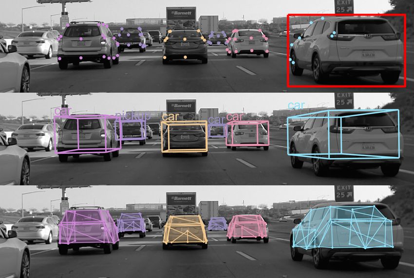
quently achieves more robust and accurate performance in
the erroneous cases and a more complex problem (e.g., joint
pose and shape estimation [26, 36, 45]).

2. Related Works
    As mentioned above, the PnP problem in the data con-
taining outliers is handled with REPPnP [9] or usually
the RANSAC scheme [10] where P3P [12, 25, 37] or
P4P [1, 18] are incorporated for providing minimal solu-              Figure 1: A flow chart of the proposed method for pose
tions of the PnP problem. Except for them, the existing               estimation
PnP algorithms have aimed at improving the performance in
noisy data. The PnP algorithms are traditionally categorized          some methods [8, 41] utilize the uncertainty of observations
into two types of methodologies: iterative and non-iterative          on the image space. They estimate control points [8] or di-
methods.                                                              rectly a pose parameter [41] by performing maximum like-
                                                                      lihood estimation for Sampson errors reflecting covariance
    Iterative methods [6, 13, 19, 33, 34] find a globally opti-
                                                                      information of observations.
mal pose estimate by solving a nonlinear least squares prob-
lem to minimize algebraic or geometric errors with itera-
tive or optimization techniques. Among them, the method
                                                                      3. Proposed Method
proposed by Lu et al. [34] accomplishes outstanding accu-                 In this paper, we handle how to reduce the computational
racy. It reformulates an objective function as minimizing             complexity of a RANSAC-based scheme for the PnP prob-
object-space collinearity errors instead of geometric errors          lem in outlier-contaminated data. Many real-world applica-
measured on the image plane. The least squares problem is             tions [26, 36, 45] aim at estimating a 6D pose of an object
solved using the way of Horn et al. [20] iteratively. Garro et        on the ground, given 2D object bounding boxes from ob-
al. [13] proposed a Procrustes PnP (PPnP) method reformu-             ject detectors [15, 31]. The additional information is not
lating the PnP problem as an anisotropic orthogonal Pro-              only useful to reduce the number of required points for
crustes (OP) problem [7]. They iteratively computed a so-             solving the PnP problem but also acquired without an ex-
lution of the OP problem by minimizing the geometric er-              tra computational loss since it is already given in some ap-
rors in the object space until convergence, which achieved            plications. Hence, we propose a perspective-1-point (P1P)
a proper trade-off between speed and accuracy.                        method for an object on the ground, which significantly
    On the other hand, non-iterative methods [17, 24, 28,             raises the speed of the RANSAC-based scheme. In the fol-
29, 47, 48] quickly obtain pose estimates by calculating              lowing sections, we first introduce a general framework for
solutions of a closed form. Lepetit et al. [28] proposed              n-point RANSAC-based pose estimation, then propose the
an efficient and accurate method (EPnP) for solving the               P1P method for roughly estimating an object pose using one
PnP problem with computational complexity of O(n). They               point sample, and finally suggest a novel robust estimation
defined the PnP problem as finding virtual control points,            method for polishing the rough pose estimate.
which was quickly calculated by null space estimation of a            3.1. General framework of n-point RANSAC-based
linear system. They refined the solution with the Gauss-                    pose estimation
Newton method so that its accuracy amounted to that of
                                                                          We employ a general framework for n-point RANSAC-
Lu et al. [34] with less computational time. Hesch et al. [17]
                                                                      based pose estimation.1 Given a set of 2D-3D keypoint cor-
formulated the PnP problem as finding a Cayley-Gibbs-
                                                                      respondences, C, we sample n keypoint correspondences,
Rodrigues (CGR) parameter by solving a system of sev-
                                                                      i.e., {(x1 , X1 ), ..., (xn , Xn )|(xi , Xi ) ∈ C}, and compute a
eral third-order polynomials. Several methods [24, 47, 48]
                                                                      pose candidate Tcand using a PnP algorithm. Then the re-
employ quaternion parameterization and solve a polynomial
                                                                      projection errors are computed for all the keypoint corre-
system minimizing algebraic [47, 48] or object-space [24]
                                                                      spondences and the keypoints whose reprojection errors are
errors with the Gröbner basis technique [27]. In particular,
                                                                      within a threshold tin are regarded as inliers. This process
the method of Kneip et al. [24] results in minimal solutions
                                                                      is repeated N times and we select the pose with the maxi-
of the polynomial system and is generalized for working on
                                                                      mum number of inliers as the best pose estimate. The maxi-
both central and non-central cameras. Li et al. [29] pro-
                                                                      mum number of iteration, N , can be reduced by the adaptive
posed a PnP approach robust to special cases such as planar
                                                                      RANSAC technique [10] which adjusts N depending on the
and quasi singular cases. They defined the PnP problem by
                                                                      number of inliers during the RANSAC process. Finally, the
finding a rotational axis, an angle, and a translation vector,
and solved the linear systems formulated from projection                1 Please find a flowchart of the RANSAC-based scheme in the supple-

equations and a series of 3-point constraints [38]. Recently,         mentary material.

                                                                  2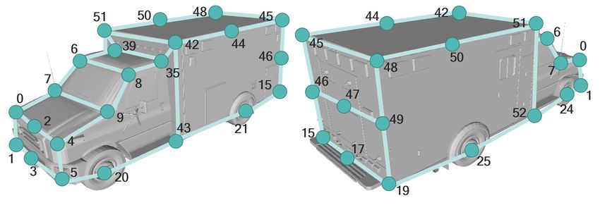
Case 1             Case 2
                       Case 1        Case 2         Case 3       Case 4
         (a)                                  (b)

Figure 2: Case study on the 1-point object pose estimation:
(a) 3DBB of an object in the BEV and (b) four cases of the                                                                 Case 3             Case 4
pose estimation depending on the yaw angle                                                       (a)                                   (b)

pose estimate is polished by minimizing the reprojection er-                      Figure 3: Parameter definition in the BEV: (a) parameters in
rors of the inlier keypoints or using the existing PnP algo-                      the camera coordinate system and (b) parameters for each
rithms.                                                                           case in the 3D model coordinate system

3.2. Perspective-1-point solution                                                 corners of the 3DBB depending on the yaw angle of the ob-
    To reduce the number of points required for comput-                           ject, e.g., in Case 1, the left and right edges of the 2DBB
ing an object pose hypothesis, we need to use some prior                          are paired with Corners 4 and 2 of the 3DBB, respectively.
knowledge. First, we assume that the tilt of a camera to the                      In this way, we can find out the four cases3 for the 1-point
ground where an object of interest is placed is given as a                        pose estimation and will describe how to compute an object
pitch angle θp .2 From the pitch angle, a rotation transfor-                      pose using a point correspondence at each case.
mation Rcg ∈ SO(3) from the ground to the camera is de-                               Figure 3 shows the definition of the parameters required
fined as Rcg = eωp where ωp = [−θp , 0, 0]> ∈ so(3) and                           to formulate an equation in the BEV. In Figure 3a, vK (ma-
e : so(3) 7→ SO(3) is an exponential map. For example,                            genta) is a directional vector from the camera center to the
if an object is fronto-parallel to the image plane, Rcg = I3                      keypoint, vL and vR (green) are the back-projected rays of
where I3 is a 3 × 3 identity matrix. Second, besides the                          the left and right edges of the 2DBB4 , respectively, vO (red)
3D model of the object and its 2D-3D keypoint correspon-                          is the forward direction of the object, vC (dark green) is the
dence, which are provided as input by default in the PnP                          forward direction of the camera, φy , θL , and θR are angles
problem, we assume that the 2D bounding box (2DBB) of                             between vC and vK , vK and vL , and vK and vR , respec-
the object of interest in an image is given as an input. Using                    tively, lC is the length between the camera center point and
the additional prior information, the problem is redefined as                     the keypoint, lL and lR are the lengths between the keypoint
aligning the projection of the 3D bounding box (3DBB) into                        and the corners of the 3DBB, and φL and φR are angles be-
the back-projected rays of both the side ends of its 2DBB in                      tween vL and lL , and vR and lR , respectively. In Figure 3b,
a bird-eye view (BEV), thereby computing the yaw angle                            ψL and ψR are angles between the forward direction of the
of the object and the depth of the keypoint as shown in Fig-                      object and the corners of the 3DBB. Then our goal is to
ure 1b. Here, we formulate an equation that computes the                          compute a local yaw angle of the object, i.e., an angle be-
pose of the object of interest by 1-DoF parameterization. A                       tween vK and vO , θy , and a depth from the camera center
unique pose hypothesis per keypoint is obtained by solving                        to the keypoint, lC .
the equation. Consequently, through the RANSAC process,
                                                                                      We first describe the 1-point pose estimation method for
we find the best pose parameter with the maximum num-
                                                                                  Case 1. We can derive an equation to compute θy from the
ber of inliers among these hypotheses and then optimize the
                                                                                  sine rule as follows:
pose.
    There are four cases of the 1-point object pose estima-                                                   lR sin φR   lL sin φL
tion depending on the yaw angle of the object as shown in                                              lC =             =           ,                     (1)
                                                                                                                sin θR      sin θL
Figure 2. In Figure 2a, the red arrow and the blue rectangle
denote the forward direction of the object and the 3DBB in                        where φR = θy + ψR − θR and φL = −θy − ψL − θL . From
the BEV, respectively. We denote the four corners of the
3DBB by numbers which will be used in Figure 3b. In Fig-                              3 In fact, the number of the cases are exactly more than 4 due to the

ure 2b, the green rectangle and the blue hexahedron denote                        perspective effect, e.g., Corners 3 and 4 of the 3DBB are possible to be
the 2DBB of the object and the projection of the 3DBB to                          adjacent to the 2DBB, but those cases can approximate to one of the cases
                                                                                  in Figure 2b if an object of interest is far enough from the camera.
an image, respectively. Then, as shown in Figure 2b, the                              4 We assume that the side edges of the 2DBB are back-projected to the
left and right edges of the 2DBB are adjacent to two of the                       planes perpendicular to the ground so the projections of the planes into the
                                                                                  ground become the rays passing through the camera center and the corners
  2 It   is pre-calibrated or calculated in an online manner with [22, 46].       of the 3DBB.

                                                                              3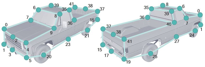
Table 1: Range of angle parameters for the four cases Xi in the ASM is defined by summing a mean location X̄i
and the combinations of M basis vectors Bji .
Parameter Case 1 Case 2 Case 3 Case 4
π π π M
−π, − π2
− ,0
X
θy 0, 2 ,π
π2 π2 Xi = X̄i + λj Bji , (5)
−π, − π2
π
ψL ,π − ,0 0, 2 j
π 2π π2
−π, − π2
ψR 0, 2 −2,0 2
,π
where λ = {λ1 , ..., λM } is a set of variables depending on
shape variation.
Eq. 1, the yaw angle θy is derived as Then the object pose and shape are jointly estimated by
minimizing residuals ri (reprojection errors) as follows:
(ψR −θR )
− lR sinsin lL sin (ψL +θL )
!
θR − sin θL |C|
θy = arctan lR cos (ψR −θR ) lL cos (ψL +θL )
, (2) X
+ argmin ρ(ri (T, λ)), (6)
sin θR sin θL T,λ i=0
and the depth of the keypoint, lC , is calculated using PM
where ri (T, λ) = kf (R(X̄i + j=0 λj Bji ) + t) − xi k2 ,
Eq. (1).5
|C| is the cardinality of the correspondence set C, the ob-
Once θy and lC are calculated, an object pose Tco ∈ ject pose T is represented by decomposition into a rotation
SE(3), which is a transformation matrix from the object matrix R and a translation vector t, f is a projection func-
coordinates to the camera coordinates, can be computed by tion from a 3D coordinate to an image coordinate, and ρ
represents an M-estimator [21] for robust estimation in the
Rcg 03 eωy lC dx I3 −X
Tco = , (3) presence of outliers.
0>
3 1 0>
3 1 0>
3 1
In our experiments, we use the Tukey biweight function
where ωy = [0, φy + θy , 0]> , X is a 3D location of the defined by
selected keypoint, and dx is a normalized directional vector
i
c2 1 − 1 − ri 2 3 ,
h
by back-projecting the keypoint x to a 3D ray. Here, dx can if ri ≤ c and
ρ(ri ) = 6 c
be computed by c 2
6 , if ri > c.
(7)
R> K−1
x̂ 1 0 0
cg Here, c = 4.685s where a scale factor s is
dx = q , where S = 0 0 0 ,
M AD(ri )/0.6745. M AD(ri ) means a median absolute
x̂ K Rcg SR>
> −>
cg K −1 x̂
0 0 1
deviation of residuals ri . We initialize the coefficients λ as
(4) zeros and the object pose by the RANSAC process where
where K is a camera intrinsic matrix and x̂ is the homoge- the unknown 3D model is substituted with the mean shape
neous coordinate of x. X̄. Finally, optimal pose and shape minimizing Eq. (6)
The object poses for the other cases are similar to Case are estimated using the iterative reweighted least squares
1 in terms of computation. The only difference is the defi- (IRLS) method.
nitions of ψL and ψR as shown in Figure 3b. Due to all the However, the common approach [32] for robust pose
cases presented in Figure 2 and the sign inside the arctan- and shape estimation often gets stuck in local minima by
gent function of Eq. B.10, we have four solutions. However, the following reasons: First, the scale factor computed by
as shown in Table B.1, if we consider the ranges of θy , ψL , MAD attains a breakdown point of 50% in a statistical point
and ψR for each case, we can filter out unreliable solutions of view but does not produce a geometrically meaningful
and obtain a unique solution from only one keypoint. threshold in the data contaminated with outliers. Second,
3.3. Hierarchical robust pose estimation of objects the M-estimator is sensitive to initial parameters. In partic-
with deformable shapes ular, our P1P solution produces a more noisy pose estimate
when the camera pitch angle varies or a 2D bounding box
Many practical applications [4, 26, 36, 45] have dealt
from an object detector is erroneous.
with the pose estimation of objects with deformable shapes.
Inspired by MM-estimator [44] and annealing M-
Unlike solving the PnP problem using a known 3D model,
estimator [30] that reduce the sensitivity to the scale esti-
estimating object pose and shape simultaneously in a sin-
mate and avoid to get stuck in a local minimum via an an-
gle image is an ill-posed problem. Thus, the existing
nealing process, we propose a hierarchical robust estimation
methods [4, 26, 36, 45] have exploited active shape mod-
method for the object pose and shape estimation. We repeat
els (ASM) [5]. Given a set of class-specified 3D object
M-estimation while decreasing the scale factor. Here, we
models as prior information, the ith 3D keypoint location
use geometrically meaningful and user-defined scale fac-
5 Please see the supplementary material for the details of the derivation. tors because the threshold empirically set by a user may be
4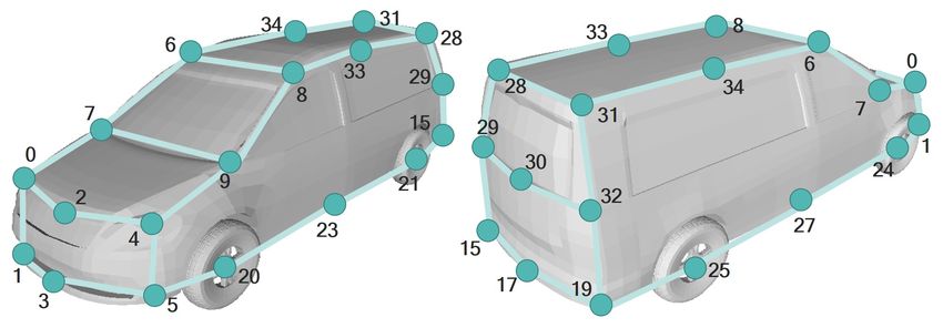
Algorithm 1 Hierarchical robust pose and shape estimation              ing box errors from -5 pixels to 5 pixels are added to 2D
Require: C, Tinit , τ1 , τ2 , τ3                                       bounding box observations.
Ensure: T, λ
 1: T ← Tinit , λ ← 0                                                  4.1.2 Evaluation metric
                    P|C|
 2: T ← argminT i ρ(ri (T|λ = 0)|c = 4.685γ(s|τ2 , τ3 ))               We use mean rotation and translation errors which have
                          P|C|
 3: T, λ ← argminT,λ i ρ(ri (T, λ)|c = 4.685γ(s|τ1 , τ2 ))             been widely used in the literature [9, 47, 48]. Given a rota-
 4: Cinlier ← {(xi , Xi )|ri (T, λ) < τ1 }                             tion estimate R and a translation estimate t, the translation
                          P|C      |
 5: T, λ ← argminT,λ i inlier kri (T, λ)k2                             error is measured by et (%) = ktgt − tk/ktk × 100 and
                                                                       the rotation error by er (◦ ) = max3i=1 {arccos (rgt,i · ri ) ×
                                                                       180/π} where rgt,i and ri are the ith column of the rotation
rather meaningful than one calculated from statistical anal-           matrices Rgt and R. For each experiment, we calculated
ysis in the case that camera properties such as intrinsic pa-          mean errors of 1000 independent simulations. The methods
rameters remain constant and the input data contain outliers.          were tested on a 3.4GHz single core using MATLAB.
    The details of the proposed method are described in Al-
gorithm 1. Given the 2D-3D correspondence set C, an ini-               4.1.3   Variation of the outlier ratio and the number of
tial pose Tinit by the RANSAC process, and user-defined                        points
thresholds τ1 , τ2 , and τ3 (τ1 < τ2 < τ3 ), the object pose           Our 1-point RANSAC-based method (RNSC-P1P) is com-
T and shape λ are estimated through three stage optimiza-              pared with RANSAC+P3P [10, 25] (RNSC-P3P) and
tion. At the first stage, the roughly initialized pose is re-          REPPnP [9]. In addition, their results are polished by the
fined with the scale estimates loosely bounded to a range of           Gauss-Newton (GN) method or several PnP approaches:
[τ2 , τ3 ] by the function γ, which is a clamp function for lim-       EPnP [28], RPnP [29], ASPnP [48], OPnP [47], and
iting the range of an input value x to [α, β] and defined as           EPPnP [9].6 In all the experiments, the inlier threshold of
γ(x|α, β) = max(α, min(x, β)). At the second stage, the                RANSAC is set to tin = 4 pixels and the algebraic error
pose T and shape parameter λ are jointly optimized with                threshold of REPPnP is set to δmax = ktin /f where a con-
the scale estimates tightly bounded to a range of [τ1 , τ2 ].          stant k = 1.4 and the focal length f = 800 as recommended
Finally, the pose and shape are polished using only the in-            in [9].
lier correspondences set Cinlier . The first and second stages             Figures 4a and 4b show the mean rotation and translation
are computed using the IRLS method and the third stage                 errors in E1. It demonstrates that RNSC-P1P (or RNSC-
is done using the Gauss-Newton method. In a case of the                P1P+PnP strategies) is superior to RNSC-P3P (or RNSC-
PnP problem using a known 3D model, the hierarchical ro-               P3P+PnP strategies). Since E1 has no pitch angle error and
bust estimation method can be also used to estimate only an            P1P uses the 1-DoF rotation parameterization constrained
object pose by excluding λ in Algorithm 1.                             by prior pitch information, the pose estimates of P1P are
                                                                       more accurate than those of P3P in this experiment. Hence,
4. Experiments                                                         the number of inliers by P1P is higher than that by P3P as
4.1. Synthetic experiments                                             shown in Figure 4c. Figures 4d and 4e represent the re-
                                                                       sults in E2, which show the same tendency as the results
4.1.1 Dataset                                                          of E1. REPPnP achieved better accuracy than our method
It is assumed that a camera is calibrated with a focal length          because it took much more inliers by using the loose thresh-
of 800 pixels and images are captured with resolution of               old. However, REPPnP frequently produced invalid object
640 × 480. Object points are randomly sampled with a uni-              pose estimates in 1) the case that outlier ratio was more than
form distribution in a cube region of [−2, 2] × [−2, 2] ×              50% and 2) the case that a small number of point correspon-
[−2, 2]. A center location and a yaw angle of an object                dences were used, e.g., the number of points is less than 200
are randomly sampled from a region of [−4, 4] × [−1, 1] ×              as shown in Figures 4d and 4e, because of the effect of the
[20, 40] and a range of [−π, π], respectively, and used to             high outlier ratio of 50%. On the other hand, RANSAC-
calculate the ground truth rotation matrix Rgt and transla-            based methods consistently provide valid pose estimates de-
tion vector tgt . We extract 300 object points and generate            spite the high outlier ratio of 90%.
2D image coordinates by projecting them onto the image                     As shown in Figures 4g and 4i, our RNSC-P1P-based
plane. Then Gaussian noise of σ = 2 pixels is added to the             methods take much less iterations than RNSC-P3P-based
image coordinates. The pitch angle of a camera and a ratio             methods. Consequently, Figures 4h and 4j show that the
of outliers are set to 0◦ and 50%, respectively. We design             computational time of RNSC-P1P-based methods is con-
4 types of experiments. (1) E1: the outlier ratio is changed           siderably faster than that of RNSC-P3P-based methods but
from 10% to 90%. (2) E2: the number of object points is                slower than that of REPPnP.
changed from 50 to 1000. (3) E3: pitch angle errors from                  6 The results of EPnP and OPnP are refined by GN and the Newton (N)

−5◦ to 5◦ are added to the camera pose. (4) E4: 2D bound-              method, respectively.

                                                                   5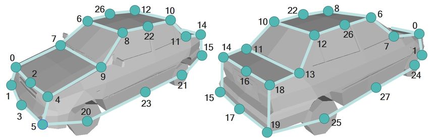
(a)                                 (b)                                    (c)

                          (d)                                 (e)                                    (f)

                    (g)                        (h)                            (i)                          (j)

                    (k)                         (l)                          (m)                           (n)

Figure 4: Results of synthetic experiments E1-E4. (a), (b), (c), (g), and (h) ((d), (e), (f), (i), and (j)) represent the mean
rotation errors, the mean translation errors, the mean number of inliers, the mean number of iteration of RANSAC, and the
computational time on E1 (E2), respectively. (k) and (l) ((m) and (n)) represent the mean rotation errors and the number of
inliers on E3 (E4), respectively. Please see the supplementary material for high-quality images.

4.1.4 Pitch angle and bounding box errors                           ter performance than the RNSC-P3P-based methods if the
Since the proposed method assumed a fixed pitch angle and           pitch error is within 1.5 degrees or the bounding box error
used a 2D bounding box as additional information, we per-           is within 2 pixel, otherwise their performance is degraded.
formed E3 and E4 to analyze the effect of the pitch angle
and bounding box errors on our method. Figures 4k-4n                4.1.5   Hierarchical robust estimation
show that both the pose estimation accuracy and the number          As mentioned in Section 3.3, the hierarchical robust esti-
of inliers decrease as the pitch angle and bounding box er-         mation (HRE) method can be used in pose estimation us-
rors increase. The RNSC-P1P-based methods produce bet-              ing known 3D models. We compared RNSC-P1P+HRE

                                                              6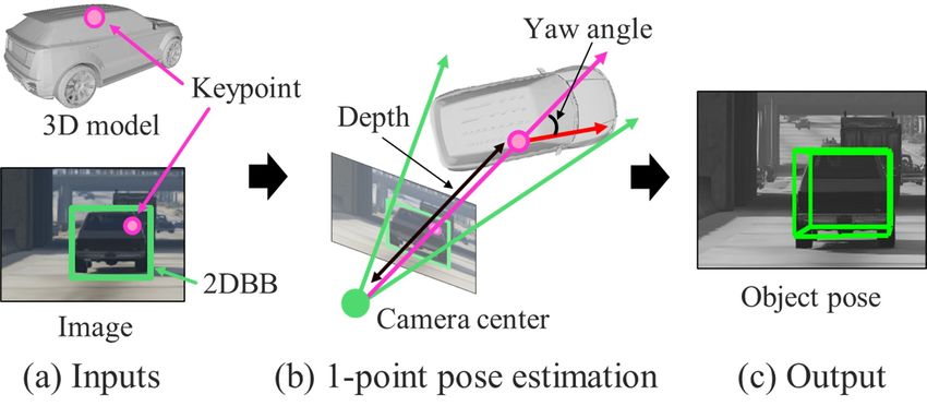
(a)                           (b)                              (c)                                   (d)
Figure 5: Results of our hierarchical robust estimation method. (a) and (b) ((c) and (d)) represent the mean rotation errors
and the number of inliers on E3 (E4), respectively.

with RNSC-P1P+GN in E3 and E4. In the experiments,                    Table 2: Speed and accuracy trade-offs of various keypoint
the parameters τ1 , τ2 , and τ3 are set to 4, 6, and 12 pix-          detection networks.
els, respectively. As shown in Figures 5b and 5d, RNSC-
                                                                                                            Vertex err.      Latency
P1P+HRE produces the consistently higher number of in-                         Model         Class acc.                 GMAC
                                                                                                             (pixel)          (ms)
liers than RNSC-P1P+GN in spite of the effect of pitch an-
gle and bounding box errors. It demonstrates that the scale            Res50 256 × 192           0.997           5.24         5.45      13.54
estimates of HRE are appropriately bounded by manually                 Res10 256 × 192           0.990           7.12         2.32       5.84
                                                                       Res50 128 × 96            0.993           7.57         1.36      7.31
determined but geometrically meaningful thresholds at each
                                                                       Res10 128 × 96            0.986          10.05         0.50      3.03
stage. Consequently, HRE converges to a global minimum
even if an initial pose estimate is noisy, whereas the existing       Table 3: Rotation, translation, and vertex errors for the ex-
estimator converges to local minima, as shown in Figures 5a           periments on known models (G1) and ASM (G2). Bold and
and 5c.                                                               italic mean the best and the second best, respectively.
4.2. Experiments on a virtual simulation dataset
                                                                                   Known models (G1)               ASM (G2)
4.2.1 Dataset                                                          Model
                                                                                   RNSC-P1P RNSC-P3P               RNSC-P1P          RNSC-P3P
To evaluate our method in a real application, we generated
                                                                                   GN HRE GN HRE                   RE         HRE RE      HRE
a dataset from a virtual driving simulation platform. We
defined 53 keypoints for 4 types of vehicles (i.e., car, bus,                er    3.78   1.56   1.90    1.41   er 2.98 2.20 3.68         2.77
                                                                       Res10
                                                                             et    6.28   1.61   1.76    1.30   ev 30.53 21.16 23.08      21.28
pickup truck, and box truck) in a similar manner with [39].                  e     3.76   1.19   1.46    0.96   er 2.57 1.96 3.16         2.43
Then we generated 2D corresponding keypoints by project-               Res50 r
                                                                             et    6.38   1.36   1.41    0.93   ev 21.43 21.23 22.18      20.77
ing them using ground truth poses. Ground truth bounding
boxes of objects were calculated from 2D projection of the            tions, we used two ResNets (Res50 and Res107 ) as back-
3D vehicle models. The pitch angle θp of the camera was               bones and two resolutions (256 × 192 and 128 × 96) as in-
set to 0◦ as prior information. However, since the camera             put sizes. More complicated network architectures [3, 40]
of the ego-vehicle was considerably shaking and the road              can boost the detection performance further, but is out of
surface was often slanted, the pitch angle was regarded to            scope of this paper. To compare the speed of each model,
be very noisy. Images were captured with image resolution             we measured FLOPS and inference speed of models on
of 1914 × 1080 pixels and a horizontal FOV of 50.8◦ . In to-          Qualcomm® SnapdragonTM8 SA8155P’s DSP unit. All
tal, we captured 100,000 frames including 207,977 objects             models were trained by using Adam optimizer [23] with 90
which were split into 142,301, 10,997, and 54,679 instances           epochs and the learning rate was divided by 10 at 60 and
for training, validation, and testing, respectively.                  80 epochs with the initial learning rate of 0.001 and weight
4.2.2 Keypoint detection                                              decay was set to 0.0001. We applied the softargmax to de-
                                                                      termine the location of each keypoint. Table 2 shows the
To detect objects’ keypoints, we employ a network archi-
                                                                      comparison of the accuracy and speed among these models.
tecture similar to [42]. Specifically, we train ResNets[16]
on top of which three to four transposed Conv-BN-ReLU                 4.2.3 Evaluation
blocks are stacked to upscale output feature maps. These              We performed two types of experiments: (1) G1: object
networks take a cropped object image as input and have two            pose estimation using known 3D object models and (2) G2:
output heads: one outputs prediction maps whose number                object pose and shape estimation using ASM. In G1, we
of channels equals to the maximum number of pre-defined                  7 Res10 models simply remove a residual block in each stage
keypoints of all classes; the other predicts the label of the         (conv2∼conv5) of Res18.
object class of the input. To investigate the speed and ac-              8 Qualcomm® SnapdragonTM is a product of Qualcomm Technologies,

curacy trade-offs on various backbones and input resolu-              Inc. and/or its subsidiaries.

                                                                  7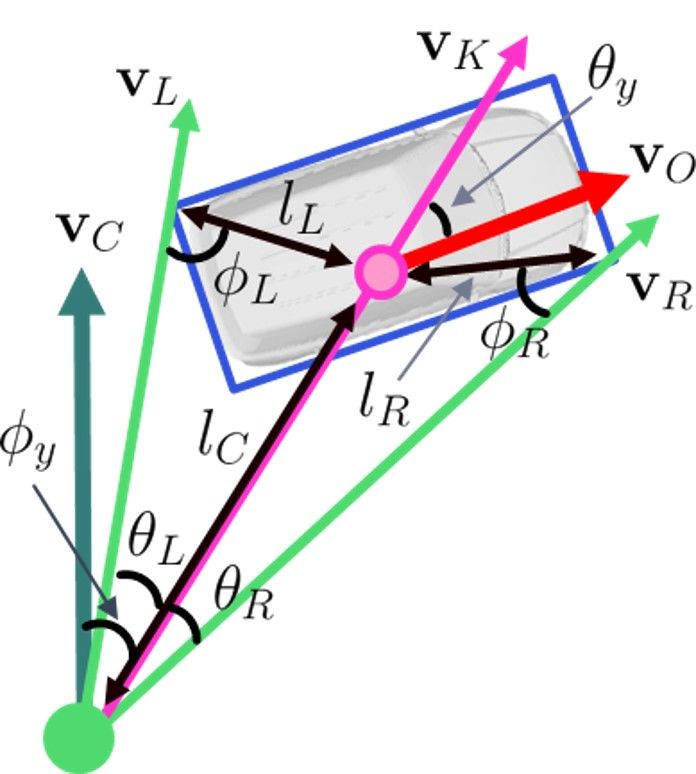
evaluate RNSC-P1P and RNSC-P3P with GN and HRE, re- Table 4: Rotation and translation errors for the experiments
spectively, and measure the average rotation and translation on the KITTI validation set. Each value represents an error
errors. In G2, we take the same protocol with G1 but substi- at the easy/moderate/hard case.
tute GN with the robust estimation (RE) method of Eq. (6)
Method er (◦ ) ea (◦ )
and additionally measure average vertex error ev (cm) be-
tween ground truth and reconstructed 3D models whose RNSC-P1P+RE 3.203/4.141/4.283 0.1376/0.1509/0.1531
scales are adjusted using a scale difference between ground RNSC-P1P+HRE 3.365/4.016/4.071 0.1356/0.1450/0.1460
truth and estimated translation vectors because of its scale RNSC-P3P+RE 4.083/5.482/5.450 0.1511/0.1651/0.1644
RNSC-P3P+HRE 4.021/5.243/5.231 0.1472/0.1616/0.1613
ambiguity. In the experiments, the ground truth 2D bound-
ing boxes were used and the parameters tin , τ1 , τ2 , and τ3
were set to 0.0375l, 0.0375l, 0.05l, and 0.15l, respectively,
where l = max(wo , ho ) and wo and ho were width and
height of a 2D object bounding box. Table 3 presents the
results for the experiments. It shows that the performance
of HRE is superior to those of both GN and RE. In G1,
RNSC-P3P-based methods are more accurate than RNSC-
P1P-based methods due to pitch errors. Nevertheless, the
performance of RNSC-P1P+HRE surpasses that of RNSC-
P3P+GN by virtue of securing more valid inliers by HRE.
G2 is a more difficult scenario because the pose should
be calculated from an inaccurate 3D model, i.e., the mean
shape of ASM. Contrary to G1, RNSC-P1P-based methods (a) (b)
achieve better rotational accuracy as the constrained pitch Figure 6: Results of RNSC-P1P+RE(a) and RNSC-
angle rather restricts the range of a rotation estimate in the P1P+HRE(b). Top, middle, and bottom images represent
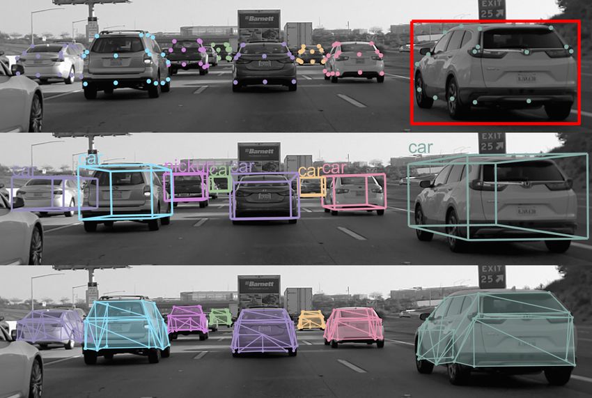
early optimization stage with large shape variation. 2D projection of inlier keypoints, 3D bounding boxes, and
shape reconstruction results using ASM, respectively.
4.2.4 Computational time
We tested the proposed method, i.e., RNSC-P1P+HRE with
the keypoint detection model of Res10-128×96 on the DSP the average angular error between t and tgt as a transla-
unit. Given a 2D object bounding box, the pose and shape tion error ea (◦ ) according to [43]. As shown in Table 4,
estimation took 4.38 ms per object where RNSC-P1P+HRE RNSC-P1P+HRE achieves the best performance in most
took 0.15 ms on CPU, keypoint detection took 3.03 ms on cases. Figure 6 shows the results of RNSC-P1P+RE and
DSP, and the pre- and post-processing, such as normaliza- RNSC-P1P+HRE from an input image captured in a real-
tion, image cropping and resizing, and softargmax opera- world scene. In the red box of Figure 6a, RNSC-P1P+RE
tion for keypoint extraction, took the rest of the computa- reconstructed the shape of the vehicle incorrectly, whereas
tional time. RNSC-P1P+HRE estimated its shape completely with more
4.3. Experiments on real-world datasets inlier keypoints. It demonstrates that the proposed method
4.3.1 Experimental setting works well in practical applications that require to detect
We used the KITTI object detection dataset [14] to evaluate objects with arbitrary shape under abrupt pitch angle varia-
quantitatively our method in real-world scenes. Following tion by a shaking camera.
the protocol of [2], we split the KITTI training data into
the training and validation sets. From the training set, we
selected 764 and 1019 instance samples for training and val- 5. Conclusion
idation of the keypoint detection network, respectively. We In this paper, we proposed an efficient method based
manually annotated keypoints and then trained the model on 1-point RANSAC to estimate a pose of an object on
of Res50 256 × 192. In addition, we captured images in a the ground. Our 1-point RANSAC-based method using
real-world scene to qualitatively compare the methods. 2D bounding box prior information was much faster than
the conventional method such as RANSAC+P3P by sig-
4.3.2 Evaluation nificantly reducing the number of trials. In addition, our
We evaluate RNSC-P1P and RNSC-P3P with RE and HRE, hierarchical robust estimation method using geometrically
respectively, on the validation set by measuring rotation meaningful and multiple scale estimates produced superior
and translation errors as in Section 4.2. However, since results in the evaluation using synthetic, virtual driving sim-
the translation estimate has scale ambiguity, we employ ulation, and real-world datasets.
8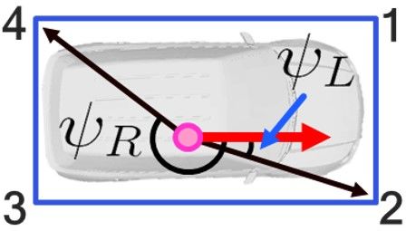
References                                                              [18] Radu Horaud, Bernard Conio, Olivier Leboulleux, and
                                                                             Bernard Lacolle. An analytic solution for the perspective 4-
 [1] Martin Bujnak, Zuzana Kukelova, and Tomas Pajdla. A gen-                point problem. Computer Vision, Graphics, and Image Pro-
     eral solution to the p4p problem for camera with unknown                cessing, 47(1):33–44, 1989. 1, 2
     focal length. In CVPR, 2008. 1, 2                                  [19] Radu Horaud, Fadi Dornaika, Bart Lamiroy, and Stéphane
 [2] Xiaozhi Chen, Huimin Ma, Ji Wan, Boa Li, and Tian Xia.                  Christy. Object pose: The link between weak perspective,
     Multi-view 3d object detection network for autonomous                   paraperspective, and full perspective. IJCV, 22(2):173–189,
     driving. In CVPR, 2017. 8                                               1997. 2
 [3] Bowen Cheng, Bin Xiao, Jingdong Wang, Honghui Shi,                 [20] Berthold KP Horn, Hugh M Hilden, and Shahriar Negah-
     Thomas S Huang, and Lei Zhang. Bottom-up higher-                        daripour. Closed-form solution of absolute orientation using
     resolution networks for multi-person pose estimation. arXiv             orthonormal matrices. JOSA A, 5(7):1127–1135, 1988. 2
     preprint arXiv:1908.10357, 2019. 7                                 [21] Peter J Huber. Robust statistics, volume 523. John Wiley &
 [4] Falak Chhaya, Dinesh Reddy, Sarthak Upadhyay, Visesh                    Sons, 2004. 1, 4
     Chari, M. Zeeshan Zia, and K. Madhava Krishna. Monocu-             [22] Jinyong Jeong and Ayoung Kim. Adaptive inverse perspec-
     lar reconstruction of vehicles: Combining SLAM with shape               tive mapping for lane map generation with slam. In URAI,
     priors. In ICRA, pages 5758–5765, may 2016. 4                           pages 38–41, 2016. 3
 [5] Timothy F Cootes, Christopher J Taylor, David H Cooper,            [23] Diederik P Kingma and Jimmy Ba. Adam: A method for
     and Jim Graham. Active shape models-their training and ap-              stochastic optimization. arXiv preprint arXiv:1412.6980,
     plication. CVIU, 61(1):38–59, 1995. 4                                   2014. 7
 [6] Daniel F Dementhon and Larry S Davis. Model-based object           [24] Laurent Kneip, Hongdong Li, and Yongduek Seo. UPnP:
     pose in 25 lines of code. IJCV, 15(1-2):123–141, 1995. 2                An optimal O(n) solution to the absolute pose problem with
 [7] Mohammed Bennani Dosse, Henk AL Kiers, and Jos MF                       universal applicability. In ECCV, 2014. 2
     Ten Berge. Anisotropic generalized procrustes analysis.            [25] Laurent Kneip, Davide Scaramuzza, and Roland Siegwart.
     Computational Statistics & Data Analysis, 55(5):1961–                   A novel parametrization of the perspective-three-point prob-
     1968, 2011. 2                                                           lem for a direct computation of absolute camera position and
 [8] L Ferraz, X Binefa, and F Moreno-Noguer. Leveraging fea-                orientation. In CVPR, pages 2969–2976, 2011. 1, 2, 5
     ture uncertainty in the PnP problem. In BMVC, 2014. 2              [26] J Krishna Murthy, GV Sai Krishna, Falak Chhaya, and K
 [9] Luis Ferraz, Xavier Binefa, and Francesc Moreno-Noguer.                 Madhava Krishna. Reconstructing vehicles from a single im-
     Very fast solution to the pnp problem with algebraic outlier            age: shape priors for road scene understanding. In ICRA,
     rejection. In CVPR, pages 501–508, 2014. 1, 2, 5                        2017. 1, 2, 4
                                                                        [27] Zuzana Kukelova, Martin Bujnak, and Tomas Pajdla. Auto-
[10] Martin A Fischler and Robert C Bolles. Random sample
                                                                             matic generator of minimal problem solvers. In ECCV, pages
     consensus: a paradigm for model fitting with applications to
                                                                             302–315, 2008. 2
     image analysis and automated cartography. Communications
     of the ACM, 24(6):381–395, 1981. 1, 2, 5                           [28] Vincent Lepetit, Francesc Moreno-Noguer, and Pascal Fua.
                                                                             EPnP: An accurate O(n) solution to the PnP problem. IJCV,
[11] Yasutaka Furukawa and Jean Ponce. Accurate, dense, and ro-
                                                                             81(2):155–166, feb 2009. 1, 2, 5
     bust multiview stereopsis. TPAMI, 32(8):1362–1376, 2009.
                                                                        [29] Shiqi Li, Chi Xu, and Ming Xie. A robust o(n) solution to
     1
                                                                             the perspective-n-point problem. TPAMI, 34(7):1444–1450,
[12] Xiao-Shan Gao, Xiao-Rong Hou, Jianliang Tang, and                       2012. 2, 5
     Hang-Fei Cheng. Complete solution classification for the
                                                                        [30] Stan Z. Li, Han Wang, and William Y.C. Soh. Robust es-
     perspective-three-point problem. TPAMI, 25(8):930–943,
                                                                             timation of rotation angles from image sequences using the
     2003. 1, 2
                                                                             annealing M-estimator. Journal of Mathematical Imaging
[13] Valeria Garro, Fabio Crosilla, and Andrea Fusiello. Solv-               and Vision, 8(2):181–192, 1998. 4
     ing the PnP problem with anisotropic orthogonal procrustes         [31] Wei Liu, Dragomir Anguelov, Dumitru Erhan, Christian
     analysis. In Second International Conference on 3D Imag-                Szegedy, Scott Reed, Cheng-Yang Fu, and Alexander C
     ing, Modeling, Processing, Visualization & Transmission,                Berg. Ssd: Single shot multibox detector. In ECCV, pages
     pages 262–269, 2012. 2                                                  21–37, 2016. 2
[14] Andreas Geiger, Philip Lenz, and Raquel Urtasun. Are we            [32] Manolis Lourakis and Xenophon Zabulis. Model-Based
     ready for autonomous driving? the kitti vision benchmark                Pose Estimation for Rigid Objects. In International Con-
     suite. In CVPR, 2012. 8                                                 ference on Computer Vision Systems, pages 83–92, 2013. 4
[15] Ross Girshick. Fast r-cnn. In ICCV, pages 1440–1448, 2015.         [33] David G. Lowe. Fitting parameterized three-dimensional
     2                                                                       models to images. TPAMI, 13(5):441–450, 1991. 2
[16] Kaiming He, Xiangyu Zhang, Shaoqing Ren, and Jian Sun.             [34] Chien Ping Lu, Gregory D. Hager, and Eric Mjolsness. Fast
     Deep residual learning for image recognition. In CVPR,                  and globally convergent pose estimation from video images.
     pages 770–778, 2016. 7                                                  TPAMI, 22(6):610–622, jun 2000. 2
[17] Joel A. Hesch and Stergios I. Roumeliotis. A Direct Least-         [35] Raul Mur-Artal and Juan D Tardós. Orb-slam2: An open-
     Squares (DLS) method for PnP. In ICCV, pages 383–390,                   source slam system for monocular, stereo, and rgb-d cam-
     2011. 2                                                                 eras. TRO, 33(5):1255–1262, 2017. 1

                                                                    9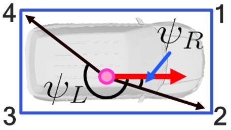
[36] J. Krishna Murthy, Sarthak Sharma, and K. Madhava Kr-
     ishna. Shape priors for real-time monocular object localiza-
     tion in dynamic environments. In IROS, pages 1768–1774,
     2017. 1, 2, 4
[37] David Nistér and Henrik Stewénius. A minimal solution to
     the generalised 3-point pose problem. Journal of Mathemat-
     ical Imaging and Vision, 27(1):67–79, 2007. 1, 2
[38] Long Quan and Zhongdan Lan. Linear n-point camera pose
     determination. TPAMI, 21(8):774–780, 1999. 2
[39] Xibin Song, Peng Wang, Dingfu Zhou, Rui Zhu, Chenye
     Guan, Yuchao Dai, Hao Su, Hongdong Li, and Ruigang
     Yang. ApolloCar3D: A large 3D car instance understanding
     benchmark for autonomous driving. In CVPR, 2019. 7
[40] Ke Sun, Bin Xiao, Dong Liu, and Jingdong Wang. Deep
     high-resolution representation learning for human pose esti-
     mation. In CVPR, pages 5693–5703, 2019. 7
[41] S Urban, J Leitloff, and S Hinz. MLPNP-A real-time maxi-
     mum likelihood solution to the perspective-n-point problem.
     In ISPRS Annals of the Photogrammetry, Remote Sensing
     and Spatial Information Sciences, 2016. 2
[42] Bin Xiao, Haiping Wu, and Yichen Wei. Simple baselines
     for human pose estimation and tracking. In ECCV, pages
     466–481, 2012. 7
[43] Jiaolong Yang, Hongdong Li, and Yunde Jia. Optimal essen-
     tial matrix estimation via inlier-set maximization. In ECCV,
     pages 111–126, 2014. 8
[44] Victor J Yohai. High breakdown-point and high efficiency ro-
     bust estimates for regression. The Annals of Statistics, pages
     642–656, 1987. 4
[45] M Zeeshan Zia, Michael Stark, Bernt Schiele, and Konrad
     Schindler. Detailed 3D representations for object recognition
     and modeling. TPAMI, 35(11):2608–2623, 2013. 1, 2, 4
[46] Daiming Zhang, Bin Fang, Weibin Yang, Xiaosong Luo, and
     Yuanyan Tang. Robust inverse perspective mapping based
     on vanishing point. In IEEE International Conference on
     Security, Pattern Analysis, and Cybernetics, pages 458–463,
     dec 2014. 3
[47] Yinqiang Zheng, Yubin Kuang, Shigeki Sugimoto, Kalle As-
     trom, and Masatoshi Okutomi. Revisiting the pnp problem:
     A fast, general and optimal solution. In ICCV, pages 2344–
     2351, 2013. 2, 5
[48] Yinqiang Zheng, Shigeki Sugimoto, and Masatoshi Oku-
     tomi. Aspnp: An accurate and scalable solution to the
     perspective-n-point problem. IEICE Transactions on Infor-
     mation and Systems, 96(7):1525–1535, 2013. 2, 5

                                                                      10
A. RANSAC-based scheme for object pose estimation
A general framework for n-point RANSAC-based pose estimation is shown in Alg. A.1.
Algorithm A.1 Pose estimation using RANSAC and a PnP algorithm
Require: C
Ensure: T
1: nbest ← 0, T ← ∅
2: for t = 1 to N do
3: Randomly sample n 2D-3D keypoint correspondences from C.
4: Tcand ← Compute a pose candidate using the PnP algorithm from the n samples.
5: ncand ← Count the number of inliers using Tcand .
6: if ncand > nbest then
7: T ← Tcand , nbest = ncand
8: end if
9: end for
10: if T 6= ∅ then
11: T ← Refine T using the inlier points.
12: end if
B. Details of perspective-1-point solution
B.1. Definition of pitch angle
Figure B.1: Definition of pitch angle
Since we want to simplify the PnP problem, we redefine the problem in the bird-eye view (BEV) in this paper. Figure B.1
shows the definition of a pitch angle θp of a camera. Once the pitch angle between the camera and the road surface is known,
a 3D directional vector Vi , i.e., a back-projected ray of a pixel on an image, is approximated to a 2D directional vector vi on
the top-view as follows.
VX
VX
vi = , where VY = R−1 cg Vi (B.1)
VZ
VZ
B.2. Parameter calculation
Many parameters9 such as φy , θL , θR , ψL , ψR , lL , and lR should be calculated prior to derivation of Eqs. (1) and (2). The
parameters φy , θL , and θR are computed as follows.
φy = arcsin vC · vK (B.2)
θL = arccos vK · vL (B.3)
θR = arccos vK · vR (B.4)
9 Please see the details of the parameters in Fig. 3.
11Let’s denote the ith corner point as pi and a selected keypoint as pK . Then, the parameters ψL , ψR , lL , and lR are
calculated depending on a case as the following table.
Table B.1: Parameter computation for the four cases
Case 1 Case 2 Case 3 Case 4
lL kpK − p4 k kpK − p3 k kpK − p1 k kpK − p2 k
lR kpK − p2 k kpK − p1 k kpK − p3 k kpK − p4 k
p4 −pK p3 −pK p1 −pK p2 −pK
ψL −acos vf · lL
acos vf · lL
−acos vf · lL
acos vf · lL
p2 −pK
ψR acos vf · lR
−acos vf · p1 −p
lR
K
acos vf · p3 −pK
lR
−acos vf · p4 −p
lR
K
B.3. Derivation of P1P solution
Here, we show the process of the derivation of Eq. (2). First of all, we prove Case 1. From the sine rule,
lL lC lR lC
= and = , (B.5)
sin θL sin φL sin θR sin φR
an equation is formulated as follows.
lR sin φR lL sin φL
lC = = (B.6)
sin θR sin θL
Because φR = θy + ψR − θR (φR > 0) and φL = −θy − ψL − θL (φL > 0), Eq. (B.6) is substituted to
lR sin (θy + ψR − θR ) lL sin (−θy − ψL − θL )
= . (B.7)
sin θR sin θL
Let ωR = ψR − θR and ωL = ψL + θL . According to the angle addition and subtraction formulae, the sine functions are
decomposed as
sin θy cos ωR + cos θy sin ωR sin θy cos ωL − cos θy sin ωL
lR = lL , (B.8)
sin θR sin θL
because ψR − θR > 0 and −ψL − θL > 0. Eq. (B.8) is reorganized with respect to sin θy and cos θy as
lR cos ωR lL cos ωL lR sin ωR lL sin ωL
sin θy + = cos θy − − . (B.9)
sin θR sin θL sin θR sin θL
Finally, we reorganize Eq. (B.9) with respect of θy as
(ψR −θR )
− lR sinsin lL sin (ψL +θL )
!
θR − sin θL
θy = arctan lR cos (ψR −θR ) lL cos (ψL +θL )
. (B.10)
sin θR + sin θL
For Cases 2-4, the local yaw angle θy is computed in the same way of Eqs. (B.5)-(B.10).
12C. Definition of keypoints
We define 53 keypoints and 4 types of vehicles: Car, Van-Bus, PickupTruck, and BoxTruck. The numbers of keypoints of
Car, Van-Bus, PickupTruck, and BoxTruck are 28, 26, 26, and 30, respectively. Some keypoints are shared among the classes.
The location and index of each keypoint are shown in Fig. C.1.
(a)
(b)
(c)
(d)
Figure C.1: Definition of keypoints of Car, Van-Bus, PickupTruck, and BoxTruck
13D. Definition of keypoints
(a) (b)
(c)
Figure D.1: High-quality images of Figs. 4(a)-4(c), i.e., the mean rotation errors, the mean translation errors, and the mean
number of inliers on E1, respectively
14(d) (e)
(f)
Figure D.2: High-quality images of Figs. 4(d)-4(f), i.e., the mean rotation errors, the mean translation errors, and the mean
number of inliers on E2, respectively
15(g) (h)
(i) (j)
Figure D.3: High-quality images of Figs. 4(g)-4(j), i.e., the mean number of iteration of RANSAC and the computational
time on E1 and E2, respectively
16(k) (l)
(m) (n)
Figure D.4: High-quality images of Figs. 4(k)-4(n), i.e., the mean rotation errors and the number of inliers on E3 and E4,
respectively
17You can also read