Real-time 3D Traffic Cone Detection for Autonomous Driving
←
→
Page content transcription
If your browser does not render page correctly, please read the page content below
Real-time 3D Traffic Cone Detection for Autonomous Driving
                                                                                Ankit Dhall, Dengxin Dai and Luc Van Gool

                                           Abstract— Considerable progress has been made in semantic
                                        scene understanding of road scenes with monocular cameras.
                                        It is, however, mainly focused on certain specific classes such as
                                        cars, bicyclists and pedestrians. This work investigates traffic
                                        cones, an object category crucial for traffic control in the con-
                                        text of autonomous vehicles. 3D object detection using images
                                        from a monocular camera is intrinsically an ill-posed problem.
arXiv:1902.02394v2 [cs.CV] 5 Jun 2019

                                        In this work, we exploit the unique structure of traffic cones and
                                        propose a pipelined approach to solve this problem. Specifically,
                                        we first detect cones in images by a modified 2D object detector.    Fig. 1. The pipeline can be subdivided into three parts: (1) object detection,
                                        Following which the keypoints on a traffic cone are recognized       (2) keypoint regression and (3) 2D-3D correspondence followed by 3D pose
                                        with the help of our deep structural regression network, here,       estimation from a monocular image.
                                        the fact that the cross-ratio is projection invariant is leveraged
                                        for network regularization. Finally, the 3D position of cones
                                        is recovered via the classical Perspective n-Point algorithm
                                        using correspondences obtained form the keypoint regression.         to safely and temporarily redirect traffic or cordon-off an
                                        Extensive experiments show that our approach can accurately          area. They may often be used for splitting or merging traffic
                                        detect traffic cones and estimate their position in the 3D world     lanes in the case of roadside construction and automobile
                                        in real time. The proposed method is also deployed on a real-
                                        time, autonomous system. It runs efficiently on the low-power        accidents. These situations need to be addressed internally
                                        Jetson TX2, providing accurate 3D position estimates, allowing       with on-board sensors because even high-definition (HD)
                                        a race-car to map and drive autonomously on an unseen                maps cannot solve this problem as the traffic cones are
                                        track indicated by traffic cones. With the help of robust and        temporary and movable.
                                        accurate perception, our race-car won both Formula Student
                                        Competitions held in Italy and Germany in 2018, cruising at
                                                                                                                It may be tempting to employ an end-to-end approach to
                                        a top-speed of 54 km/h on our driverless platform “gotthard          map directly from images to control outputs (throttle and
                                        driverless” https://youtu.be/HegmIXASKow?t=11694.                    steering commands) [15]. We, however, believe that a fusion
                                        Visualization of the complete pipeline, mapping and navigation       of part-based approaches with interpretable sub-modules and
                                        can be found on our project page http://people.ee.                   the data-driven end-to-end methods is a more promising
                                        ethz.ch/˜tracezuerich/TrafficCone/.
                                                                                                             direction. Object detection in any case is still very necessary
                                                              I. I NTRODUCTION                               for learning autonomous driving systems.
                                                                                                                It is interesting to note here that although these traffic
                                           Autonomous driving has become one of the most interest-           cones are static objects themselves, they are frequently
                                        ing problems to be tackled jointly by the computer vision,           replaced and moved around the urban driving scenario. Cars
                                        robotics and machine learning community [34], [20], [15],            may break down unexpectedly and new constructions zones
                                        [16]. Numerous studies have been done to take the field of           may pop up more often than anticipated. Although, buildings
                                        autonomous driving forward, leading to ambitious announce-           and landmarks can be mapped with ease and used for
                                        ments promising fully automated cars in a couple of years.           localization, one needs to actively detect and estimate the
                                        Yet, significant technical challenges such as the need for           position of these traffic cones for safe, automated driving.
                                        necessary robustness against adverse weather and changing
                                                                                                                A range based sensor, such as the LiDAR is designed to
                                        illumination conditions [30], [6], [35], or the capability to
                                                                                                             accurately measure 3D position, but because a LiDAR has
                                        cope with temporary, unforeseen situations such as roadside
                                                                                                             a sparse representation as compared to an image detecting
                                        construction and accidents [24] must be overcome before a
                                                                                                             small objects and predicting about their physical properties
                                        human driver can make way for autonomous driving.
                                                                                                             such as their color and texture becomes a massive challenge.
                                           Traffic control devices, such as traffic signs, traffic lights
                                                                                                             Additionally, LiDAR sensors are more expensive than cam-
                                        and traffic cones, play a crucial role in ensuring safe driving
                                                                                                             eras, driving the costs of such platform to the higher end of
                                        and preventing mishaps on the road. Recent years have
                                                                                                             the spectrum. Advances in computer vision show that images
                                        witnessed great progress in detecting traffic signs [29], [23]
                                                                                                             from even a monocular camera can be used to not only reveal
                                        and traffic lights [17], [8]. Traffic cones, however, have not
                                                                                                             what is in the scene but also where it is physically in the 3D
                                        received due attention yet. Traffic cones are conical markers
                                                                                                             world [12], [33]. Another advantage of using a monocular
                                        and are usually placed on roads or footpaths and maybe used
                                                                                                             camera is that a multi-camera setup is not required, making
                                          All authors are with ETH-Zurich adhall@ethz.ch, {dai,
                                                                                                             the system more cost-effective and maintainable.
                                        vangool}@vision.ee.ethz.ch                                              In this work, we tackle 3D position estimation and detec-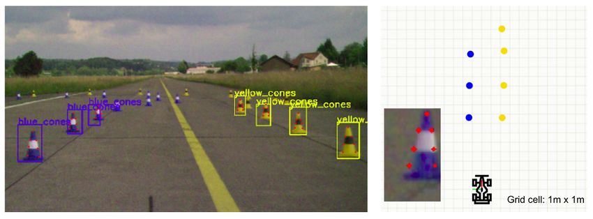
tion of traffic cones from a single image. We break the task
into three steps: 2D object detection, regressing landmark
keypoints, and finally mapping from the 2D image space to
3D world coordinates. In particular, cones are detected in
images by an off-the-shelf 2D object detector customized
for this scenario; the detected 2D bounding boxes are fed
into our proposed convolutional neural network to regress
seven landmark keypoints on the traffic cones, where the
fact that cross-ratio (Cr) is projection invariant is leveraged
for robustness. Finally, the 3D position of cones is recovered
by the Perspective n-Point algorithm. In order to train and
evaluate our algorithm, we construct a dataset of our own         Fig. 2. The left and right cameras (on the extremes) in the housing act in a
for traffic cones.                                                stereo configuration; the center camera is a stand-alone monocular camera
                                                                  and uses the pipeline elaborated in this work.
   Through extensive experiments we show that traffic cones
can be detected accurately using single images by our
method. The 3D cones position estimates deviate by only
                                                                  object boundary across 2 frames, but is limited as it is only
0.5m at 10m and 1m at 16m distances when compared with
                                                                  in simulation. Our work focuses on traffic cone detection and
the ground-truth. We further validate the performance of our
                                                                  3D position estimation using only a single image.
method by deploying it on a critical, real-time system in the
form of a life-sized autonomous race-car. The car can drive          Keypoint estimation. One of the main contributions of
at a top-speed of 54 km/h on a track flanked by traffic cones.    this work is to be able to accurately estimate the 3D pose of
   The main contribution of this paper are (1) a novel method     traffic cones using just a single frame. A priori information
for real-time 3D traffic cone detection using a single image      about the 3D geometry is used to regress highly specific
and (2) a system showing that the accuracy of our pipeline        feature points called keypoints. Previously, pose estimation
is sufficient to autonomously navigate a race-car at a top-       and keypoints have appeared in other works [31], [12].
speed of 54 km/h. The video showing our vehicle navigating        Glasner et al. [12] estimate pose for images containing cars
through a track flanked by traffic cones can be found at          using an ensemble of voting SVMs. Tulsiani et al. [33] use
https://youtu.be/HegmIXASKow?t=11694.                             features and convolutional neural networks to predict view-
                                                                  points of different objects. Their work captures the interplay
                    II. R ELATED W ORK                            between viewpoints of objects and keypoints for specific
   Fast object detection. Object detection has been one of        objects. PoseCNN [37] directly outputs the 6 degrees-of-
the most prized problems in the field of computer vision.         freedom pose using deep learning. Gkioxari et al. [11]
Moreover, for real-time, on-line performance especially on        use a k-part deformable parts model and present a unified
robotics platforms speed is of the essence. One of the first      approach for detection and keypoint extraction on people.
successful fast object detector is Viola-Jones’ face detector     Our method leverages the unique structure of traffic cones,
[36], which employs weak learners to accurately detect            more specifically the projective invariant property of cross-
faces using Haar-based features. The next class of well-          ratio, for robust keypoint estimation.
known object detectors uses deep learning in the form of
convolutional neural networks (CNNs). The string of R-                III. M ONOCULAR C AMERA P ERCEPTION P IPELINE
CNN [10], [27], [9] schemes use CNN-based features for
                                                                  A. Sensor Setup and Computation Platform
region proposal classification. YOLO [25] cleverly formu-
lates object detection as a regression task, leading to very         The experimental setup consists of 2-megapixel cameras
efficient detection systems. Single shot has been employed        (CMOS sensor-based) with a global shutter to avoid image
to 3D object detection as well [18]. While progress has been      distortion and artifacts due to fast motion. Figure 2 shows
made in terms of general object detection, the performance        our camera setup. The center camera, which is the monocular
on small-object classes such as traffic cones requires further    camera described in this work, has a 12mm lens to allow long
improvements.                                                     range perception. The left and right cameras use lenses with
   Traffic device detection. Work has been done in the            a 5.5mm focal length and act as stereo pair for triangulating
direction of detecting traffic sign [29], [23] and traffic        cones close-by. The cameras are enclosed in a customized
light [17], [8]. To aid in the efforts for bench-marking, a       3D printed, water-proof shell with polarized filters in front of
100,000 annotated image dataset for traffic signs has been        the lenses. The cameras transmit data over ethernet through
released [38]. Li et al. [21] propose a generative adversarial    a shared switch, allowing for a neat camera housing. The
network (GAN) to improve tiny object detection, such as           cameras are screwed to the metallic plate at the bottom and
distant traffic signs. Lee et al. [19] explore the idea of        are in direct contact to keep them at operating temperatures.
detecting traffic signs and output a finer mask instead of        Raw camera data is directly transmitted to a Jetson TX2
a coarse rectangle in the form of a bounding box. The work        which acts as a slave to the master PIP-39 (with Intel i7)
briefly discusses triangulation of points using the extracted     onboard “gotthard driverless”. The pipeline is light enough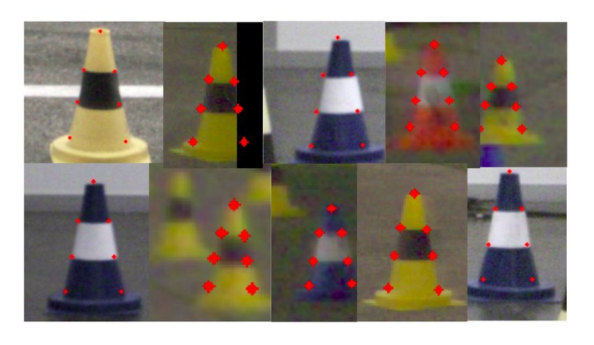
to run completely on a low-powered computing at a rate of        of interest. Doing this from a single view of the scene is
10Hz.                                                            challenging because of ambiguities due to scale. However,
                                                                 with prior information about the 3D shape, size and geometry
B. Pipeline Overview                                             of the cone, one can recover the 3D pose of detected objects
   Pose estimation from a single image is an ill-posed prob-     using only a single image. One would be able to estimate an
lem but it is solvable with a priori structural information of   object’s 3D pose, if there is a set of 2D-3D correspondences
the object of interest. With the availability of tremendous      between the object (in 3D) and the image (in 2D), along with
amounts of data and powerful hardware such as GPUs,              intrinsic camera parameters.
deep learning has proven to be good at tasks that would             To this end, we introduce a feature extraction scheme that
be difficult to solve with classical, hand-crafted approaches.   is inspired by classical computer vision but has a flavor of
Data-driven machine learning does well to learn sophisticated    learning from data using machine learning.
representations while results established from mathematics          1) Keypoint Representation: The bounding boxes from
and geometry provide robust and reliable pose estimates. In      the object detector do not directly correspond to a cone. To
our work we strive to combine the best of both worlds in an      tackle this, we extract landmark features within the proposed
efficient way holding both performance and interpretability      bounding box that are representative of the cone. In the
in high regard with a pipelined approach.                        context of classical computer vision, there are three kinds
   The sub-modules in the pipeline enable it to detect objects   of features: flat regions, edges and corners. Edges are more
of interest and accurately estimate their 3D position by         interesting than flat regions as they have a gradient in one
making use of a single image. The 3 sub-modules of the           direction (perpendicular to the edge boundary) but suffer
pipeline are (1) object detection, (2) keypoint regression and   from the aperture problem [32]. By far, the most interesting
(3) pose estimation by 2D-3D correspondence. The pipeline’s      features are the corners that have gradients in two directions
sub-modules are run as nodes using Robot Operating System        instead of one making them most distinctive among the three.
(ROS) [4] framework that handles communication and trans-           Previous feature extraction works include the renowned
mission of data (in the form of messages) between different      Harris corners detector [13], robust SIFT [22] and SURF
parts of the pipeline and also across different systems. The     [5] feature extractors and descriptors. A property that many
details will be described in more detail in Section IV.          of these possess is invariance to transformations such as
                                                                 scale, rotation and illumination, which for most use-cases
                       IV. A PPROACH
                                                                 is quite desirable. Most of these work well as general
A. Object Detection                                              feature detectors and can be used across a range of different
   To estimate 3D position of multiple object instances from     applications.
a single image, it is necessary to first be able to detect          The issue with using such pre-existing feature extraction
these objects of interest. For the task of object detection,     techniques is that they are generic and detect any kind
we employ an off-the-shelf object detector in our pipeline       of features that fall within their criteria of what a feature
in the form of YOLOv2 [26]. YOLOv2 is trained for the            point is. For instance, a Harris corner does not distinguish
purpose of detecting differently colored cones that serve as     whether the feature point lies on a cone or on a crevasse
principal landmarks to demarcate the race-track at Formula       on the road. This makes it difficult to draw the relevant
Student Driverless events (where we participated with our        2D correspondences and match them correctly to their 3D
platform). Thresholds and parameters are chosen such that        counterparts. Another issue is when a patch has a low
false positives and misclassification are minimal. For this      resolution, it may detect only a couple of features which
particular use-case, YOLOv2 is customized by reducing            will not provide enough information to estimate the 3D pose
the number of classes that it detects, as it only needs to       of an object.
distinguish among yellow, blue and orange cones each with           2) Keypoint Regression: With these limitations of previ-
a particular semantic meaning on the race-track.                 ously proposed work in mind, we design a convolutional
   Since the bounding boxes for cones have a height to width     neural network (CNN) that regresses “corner” like features
ratio of greater than one, such prior information is exploited   given an image patch. The primary advantage over generic
by re-calculating the anchor boxes used by YOLOv2 (see           feature extraction techniques is that with the help of data
[26] for details).                                               one can learn to robustly detect extremely specific feature
   Weights trained for the ImageNet [7] challenge are used       points. Although, in this work we focus on a particular
for initialization. We follow a similar training scheme as in    class of objects, the cones; the proposed keypoint regression
the original work [26]. The detector is fine-tuned when more     scheme can be easily extended to different types of objects
data is acquired and labeled during the course of the season.    as well. The 3D locations corresponding to these specific
Refer to Section V-A.1 for more details on data collection       feature points (as shown in Figure 4) can be measured in
and annotation.                                                  3D from an arbitrary world frame, Fw . For our purpose, we
                                                                 place this frame at the base of the cone.
B. Keypoint Regression                                              There are two reasons to have these keypoints located
  This section discusses how object detection in a single        where they are. First, the keypoint network regresses po-
2D image can be used to estimate 3D positions of objects         sitions of 7 very specific features that are visually distinct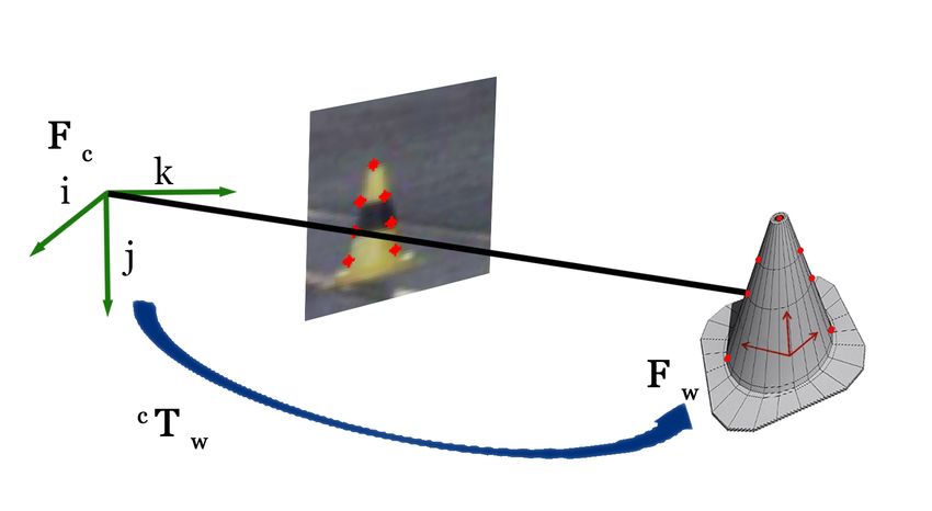
Fig. 3. Detection under varying lighting and weather conditions for yellow, blue and orange cones.
Fig. 5. Architecture of the keypoint network. It takes a sub-image patch
Fig. 4. 3D model of the cone and a representative sub-image patch with the of 80 × 80 × 3 as input and maps it to R14 , the (x, y) coordinates for the 7
image of the cone. The red markers correspond to the 7 specific keypoints keypoints. It can process 45-50 cone patches per second on a low-powered
the keypoint network regresses from a given cone patch. Jetson TX2.
accurately.
and can be considered visually similar to “corner” features. The backbone of the network is similar to the ResNet. The
Second, and more importantly, these 7 points are relatively first block in the network is a convolution layer with a batch
easy to measure in 3D from a fixed world frame Fw . For norm (BN) followed by rectified linear units (ReLU) as the
convenience Fw is chosen to be the base of the 3D cone, non-linear activation. The next 4 blocks are basic residual
enabling measurement of 3D position of these 7 points in blocks with increasing channels C ∈ {64, 128, 256, 512} as
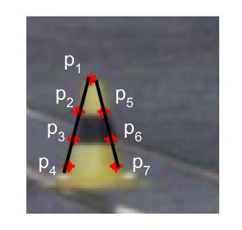
this world frame, Fw . The 7 keypoints are the apex of the depicted in Figure 5. Finally, there is a fully-connected layer
cone, two points (one on either side) at the base of the cone, that regresses the (x, y) position of the keypoints in the patch.
4 points where the center stripe, the background and the 3) Loss Function: As mentioned previously, we use
upper/lower stripes meet. object-specific prior information to match 2D-3D correspon-
The customized CNN, made to detect specific “corner” dences, from the keypoints on the image (2D) to their
features, takes as input an 80×80×3 sub-image patch which location on the physical cone (3D). In addition, the keypoint
contains a cone, as detected by the object detector, and maps network also exploits a priori information about the object’s
it to R14 . The spatial dimensions are chosen as 80 × 80, the 3D geometry and appearance through the loss function via
average size of detected bounding boxes. The output vector the concept of the cross-ratio. As known, under projective
of R14 are the (x, y) coordinates of the keypoints. transform, neither distances between points nor their ratio
The architecture of the convolutional neural network con- is preserved. However, a more complicated entity known as
sists of basic residual blocks inspired by ResNet [14] and is the cross-ratio, which is the ratio of ratio of distances, is
implemented using the PyTorch [3] framework. invariant and is preserved under a projection. While used in
As analyzed in [28], with more convolutional layers, the classical computer vision approaches that involve geometry,
tensor volume has more channels but on the other hand cross-ratio has seldom been used in the context of machine
there is a significant reduction in the spatial dimensions, learning. We use it to geometrically constrain the location
implying the tensors contain more global and high-level of the keypoints and directly integrate into the model’s loss
information than specific, local information. We eventually function.
care about location of keypoints which are extremely specific The cross-ratio (Cr) is a scalar quantity and can be
and local. Using such an architecture prevents loss of spatial calculated with 4 collinear points or, 5 or more non-collinear
information as it is crucial to predict the position of keypoints points [1]. It is invariant under a projection and the process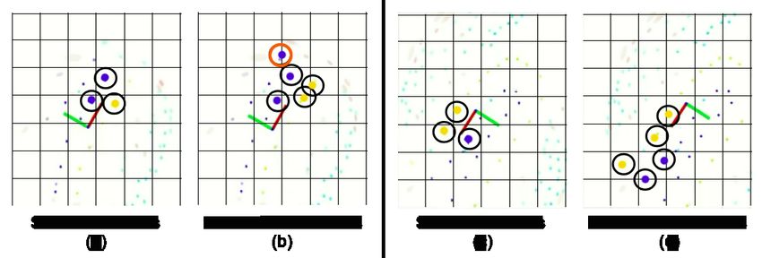
is implemented in PyTorch and used via ROS on “gotthard
                                                                                        driverless”. Refer to Section V-A.2 for more information
                                                                                        about the dataset.

                                                                                        C. 2D to 3D Correspondences
                                                                                           The keypoint network provides the location of specific
                                                                                        features on the object of interest, the keypoints. We use a
                                                                                        priori information about the object of interest (the cone,
Fig. 6. An exemplary 80×80 cone patch with regressed keypoints overlaid
                                                                                        in this case) such as its shape, size, appearance and 3D
in red. Depiction of the left (p1 , p2 , p3 , p4 ) and right arm (p1 , p5 , p6 , p7 )   geometry to perform 2D-3D correspondence matching. The
of the cone. Both of which are used to calculate the cross-ratio terms and              camera’s intrinsic parameters are available and the keypoint
minimize the error between themselves and the cross-ratio on the 3D object
(Cr3D ).
                                                                                        network provides the 2D-3D correspondences. Using these
                                                                                        pieces of information it is possible to estimate the 3D pose of
                                                                                        the object in question solely with a single image. We stitch
of acquiring images with a camera is essentially a projective                           these pieces together using the Perspective n-Point (PnP)
transform. The cross-ratio is preserved, both on the 2D                                 algorithm.
projection of the scene (the image) and in 3D space where                                  We define the camera frame as Fc and the world frame as
the object lies.                                                                        Fw . Although Fw can be chosen arbitrarily, in our case, we
   In our case, we use 4 collinear points p1 , p2 , p3 , p4 to                          choose Fw to be at the base of every detected cone, for the
calculate the cross-ratio as defined in Equation 1. Depending                           ease of measurement of the 3D location of the keypoints
on whether the value is calculated for 3D points (D = 3) or                             (with respect to Fw ) and convenience of calculating the
their projected two dimensional counterparts (D = 2), the                               transform and eventually the cone position.
distance ∆ij , between two points, pi and pj is defined.                                   We use Perspective n-Point to estimate the pose of every
                                                                                        detected cone. This works by estimating the transform c Tw
     Cr(p1 , p2 , p3 , p4 ) = (∆13 /∆14 )/(∆23 /∆24 ) ∈ R                               between the camera coordinate frame, Fc , and the world
                     q                                                          (1)     coordinate frame, Fw . As we are concerned only with the
                                 (n)     (n)
          ∆ij = ΣD         n=1 (Xi   − Xj )2 , D ∈ {2, 3}                               translation between Fc and Fw , which is exactly the position
   In addition to the cross-ratio to act as a regularizer, the                          of the cone with respect to the camera frame that we wish
loss has a squared error term for the (x, y) location of                                to estimate, in our case we discard the orientation.
each regressed keypoint. The squared error term forces the                                 To estimate the position of the cone accurately, we use
regressed output to be as close as possible to the ground-truth                         non-linear PnP implemented in OpenCV [2] which uses
annotation of the keypoints. The effect of the cross-ratio is                           Levenberg-Marquardt to obtain the transformation. In ad-
controlled by the factor γ and is set to a value of 0.0001.                             dition, RANSAC PnP is used instead of vanilla PnP, to
                                                                                        tackle and deal with noisy correspondences. RANSAC PnP
             (x)       (x)                         (y)       (y)
                                                                                        is performed on the set of 2D-3D correspondences for each
   Σ7i=1 (pi       − pi groundtruth )2 + (pi             − pi groundtruth )2            detected cone, i.e. extract the keypoints by passing the patch
                                 +γ · (Cr(p1 , p2 , p3 , p4 ) − Cr3D )2                 through the keypoint regressor and use the pre-computed
                                 +γ · (Cr(p1 , p5 , p6 , p7 ) − Cr3D )2                 3D correspondences to estimate their 3D position. One can
                                                                      (2)               obtain the position of each cone in the car’s frame by a
                                                                                        transformation between the camera frame and the ego-vehicle
   The second and third term minimize the error between                                 frame.
the cross-ratio measured in 3D (Cr3D ) and the cross-ratio
calculated in 2D based on the keypoint regressor’s output,                                      V. DATA C OLLECTION AND E XPERIMENTS
indirectly having an influence on the locations output by
                                                                                        A. Dataset Collection and Annotation
the CNN. The second term in Equation 2 represents the left
arm of the cone while the third term is for the right arm,                                 To train and evaluate the proposed pipeline data for object
as illustrated in Figure 6. For the cross-ratio, we choose                              detection and keypoint regression is collected and manually-
to minimize the squared error term between the already                                  labeled. To analyze the accuracy of the position estimates
known 3D estimate (Cr3D = 1.39408 from a real cone) and                                 using the proposed method with a single image, 3D ground-
its 2D counterpart. Equation 2 represents the loss function                             truth is collected with the help of a LiDAR.
minimized while training the keypoint regressor. The training                              1) Traffic cone detection: The object detector is trained on
scheme is explained in the following section.                                           90% of the acquired dataset, about 2700 manually-annotated
   4) Training: To train the model, Stochastic Gradient De-                             images with multiple instances of cones and performance is
scent (SGD) is used for optimization, with learning rate =                              evaluated on 10% of the data (about 300 unseen images).
0.0001, momentum = 0.9 and a batch size of 128. The                                        2) Keypoints on cone patches: 900 cone patches were
learning rate is scaled by 0.1 after 75 and 100 epochs. The                             extracted from full images and manually hand-labeled using
network is trained for 250 epochs. The keypoint regressor                               a self-developed annotation tool.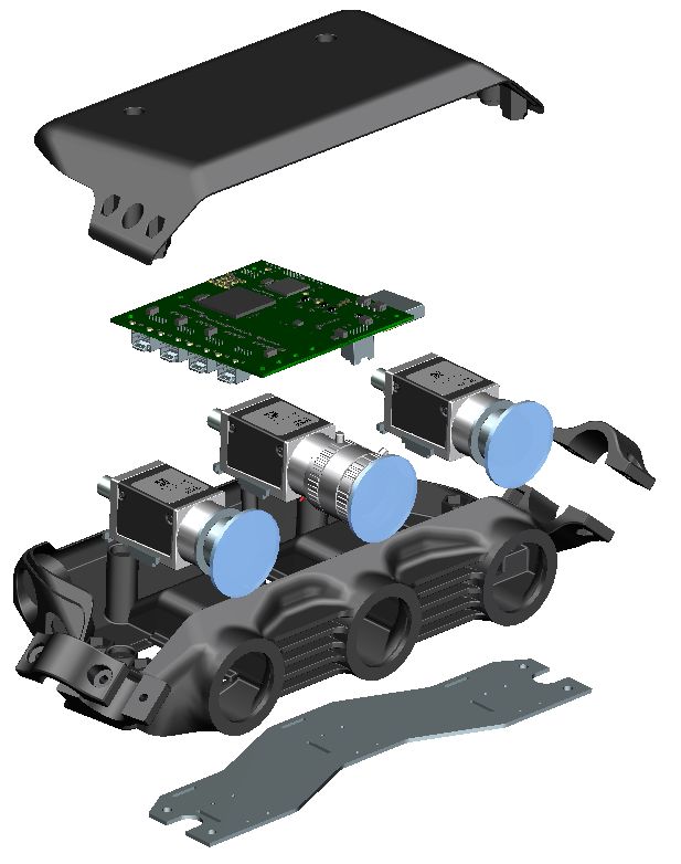
TABLE I                                                                   TABLE II
   Summary of datasets collected and manually annotated to train and                 Performance of YOLO for colored cone object detection.
  evaluate different sub-modules of the pipeline. Acronyms: (1) OtfA?:
           On-the-fly augmentation?, (2) NA: Not applicable.                                            Precision   Recall   mAP
                                                                                            Training      0.85       0.72    0.78
                  Task            Training    Testing    OtfA?                              Testing       0.84       0.71    0.76
            Cone Detection          2700        300       Yes
          Keypoint regression      16,000      2,000      Yes
          3D LiDAR position          NA         104       NA                  modules of the pipeline and handling 1 Gb/s of raw image
                                                                              data.

                                                                              B. Cone Detection
                                                                                 Table II summarizes the performance evaluation of the
                                                                              cone detection sub-module. The system has a high recall
                                                                              and is able to retrieve most of the expected bounding boxes.
                                                                              With a high precision it is averse to false detections which
                                                                              is of utmost importance to keep the race-car within track
                                                                              limits. Figure 3 illustrates the robustness of the cone de-
                                                                              tection pipeline in different weather and lighting conditions.
                                                                              The colored cone detections are shown by bounding boxes
                                                                              colored respectively. The key to driving an autonomous
                                                                              vehicle successfully is to design a perception system that has
Fig. 7. Robust performance of keypoint regression across various scenarios.
Refer to Section V-C for analysis.
                                                                              minimal or no false positives. False detections can lead to
                                                                              cone (obstacle) hallucination forcing the car off-course. The
                                                                              cone detection module is able to detect cones up to a depth
                                                                              of approximately 18-20m, however, it gets more consistent
                                                                              with cones further away due to their small size.

                                                                              C. Keypoint Regression
                                                                                 Figure 7 illustrates a montage of 10 sample patches
                                                                              regressed for keypoints after being detected by YOLOv2.
                                                                              The second cone (from the left) in the top row is detected
Fig. 8. Schematic illustrating matching of 2D-3D correspondence and
estimation of transformation between the camera frame and the world frame.    on the right edge of the image and is only partially visible
                                                                              on the image and is padded with black pixels. Even with
                                                                              missing pixels and no information about a part of the cone,
Data Augmentation. The dataset was further augmented by                       our proposed regressor predicts the keypoints. It learns the
transforming the image with 20 random transforms. These                       geometry and relative location of one keypoint with respect
were a composition of random rotations between [−15◦ ,                        to another. Even by just partially observing a cone, it
+15◦ ], scaling from 0.8x to 1.5x and translation of up to                    approximates where the keypoint would have been in case of
50% of edge length. During the training procedure, the data                   a complete image. From the examples we can see that it is
is further augmented on the fly in the form of contrast,                      able to understand spatial arrangement of the keypoints and
saturation and brightness. The final augmented annotated                      their geometry through data. For the second cone from the
dataset is partitioned to have 16,000 cone patches for training               left in the bottom row there is another cone in the background
and the remaining 2,000 cone patches for testing.                             but the keypoint network is able to regress to the more
   3) 3D ground-truth from LiDAR: In order to test the                        prominent cone. One has to note that as the dimensions of
accuracy of the 3D position estimates, corresponding object                   the bounding box become smaller, it becomes more tricky
positions measured from a LiDAR are treated as ground-                        to regress precisely due to the reduced resolution of the sub-
truth. This is done for 104 physical cones at varying distances               image as can be seen in the last two cone samples in the
from 4m up to 18m. The estimates are compared in Figure                       first row here.
9 and are summarized in Section V-D.                                             We train the model using the loss from equation 2)
   This section analyzes and discusses results of the monoc-                  which has the cross-ratio terms in addition to the mean-
ular perception pipeline, paying special attention to the                     squared term. We evaluate the performance of our keypoint
robustness of the keypoint network and the accuracy of                        regressor using the mean-squared error. The performance on
3D position estimates using the proposed scheme from a                        the train and test splits of the final keypoint regression model
single image. The keypoint network can process multiple                       is summarized in Table III. The empirical performance,
cone patches in a single frame within 0.06s, running at 15-16                 measured by the mean-squared error between the prediction
frames per second on a Jetson TX2 while running other sub-                    and ground-truth, between the train and test splits is very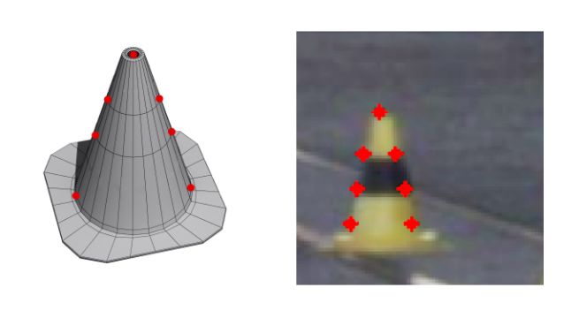
TABLE III
  Performance of the keypoint network on training and testing datasets.

                               Training    Testing
                       MSE       3.535      3.783

                                                                              Fig. 10. 3D cones using computer vision are depicted as solid yellow
                                                                              and blue circles highlighted by black circles. In the first panel, (a) & (b),
                                                                              “gotthard driverless”, shown as a coordinate frame, with red axis pointing
                                                                              forward, approaches a sharp hair-pin turn. The monocular pipeline perceives
                                                                              a blue cone on the other side of the track (marked with an orange circle),
                                                                              allowing SLAM to map distant cones and tricky hair-pins. In the second
                                                                              panel, (c) & (d), the car approaches a long straight. One can clearly see
                                                                              the difference in the range of the stereo pipeline when compared with
                                                                              the monocular pipeline which can perceive over an extended range of
                                                                              distances. With a longer perception range, the car can accelerate faster and
                                                                              consequently improve its lap-time. Each grid cell depicted here is 5m×5m.

Fig. 9. Euclidean distance between position estimates from LiDAR and
                                                                              between the ranges of the monocular and the stereo pipeline.
monocular camera pipeline for the same physical cone. The x-axis represents   Our proposed work using a monocular camera has larger
the absolute distance of the cone from the ego-vehicle frame and the y-axis   perception range than the standard triangulation solution
the Euclidean difference between the LiDAR and camera estimates. We fit
a 2nd-degree curve (shown in red) to the points. Refer to Subsection V-D
                                                                              based on stereo cameras. Additionally, the monocular camera
for details.                                                                  has a longer focal length than the stereo cameras. If the
                                                                              stereo pair also have longer focal length, the field of view
                                                                              reduces introducing blind-spots where the stereo cameras
close meaning that the network has accurately learned how                     cannot triangulate.
to localize keypoints given cone patches and does not overfit.
   Figure 7 shows the robustness and accuracy of the key-                     F. Effect of 2D bounding boxes on 3D estimates
point regressor, but it represents only the internal perfor-                     As mentioned before, we would like to see how sub-
mance of the keypoint network sub-module. In the follow-                      modules have an effect on the final 3D position estimates.
ing subsections, we analyze how outputs of intermediate                       Here, we take a step back and analyze how variability
sub-modules affect the 3D cone positions. We also show                        in output from the object detection sub-module (imprecise
how variability in output of a particular sub-module ripples                  bounding boxes) would influence the 3D positions. In this
through the pipeline and influence the final position esti-                   experiment, we randomly perturb the bounding box edges
mates.                                                                        by an amount proportional to the height and width of the
                                                                              bounding box in respective directions. Due to the inherent
D. 3D position accuracy                                                       nature of the sensor, estimating depth is most challenging
    As it is deployed on a real-time self-driving car, one of                 using raw data from cameras. Figure 11 shows how for single
the most crucial aspect is the accuracy of the estimated 3D                   images, perturbing the boxes by a certain amount (±1%,
positions. We compare the accuracy of the pipeline against                    ±5%, ±10% and ±20%) influences the variance in depth
the LiDAR’s 3D estimates, which is treated as ground-truth.                   estimates. As expected, for higher amounts of perturbation,
    Figure 9 shows data from 2 different test tracks. The x-axis              more variance in depth estimates is observed. However, even
represents the depth, in meters, of a physical cone and along                 for a ±20% perturbation, the variance is about 1 m2 at
the y-axis is the Euclidean distance between the 3D position                  15m. Figure 11 shows that even with imprecise and varying
from the LiDAR estimates and the 3D position from the                         bounding boxes, the depth of the cone is consistent and has
monocular camera pipeline. The plot consists of 104 physical                  low variance.
cones as data points. Furthermore, a second order curve is                       For additional visualizations of the detection, regression,
fitted to the data, which has mostly linear components. On                    3D position estimation, mapping and final navigation please
average, the difference is about 0.5m at a distance of 10m                    visit the project page http://people.ee.ethz.ch/
away from the ego-vehicle and only about 1m at a distance                     ˜tracezuerich/TrafficCone/
of 16m. At 5m the cone position is off by ±5.00% of its
distance, and at 16m, it is off by only ±6.25% of its distance.                                         VI. C ONCLUSION
The error is small enough for a self-driving car to drive on                     Accurate, real-time 3D pose estimation can be used for
a track flanked by cones at speeds higher than 50 km/h.                       several application domains ranging from augmented reality
                                                                              to autonomous driving. We introduce a novel keypoint
E. Extended perception range                                                  regression scheme to extract specific feature points by
  One of the goals of the method is to extend the range                       leveraging geometry in the form of the cross-ratio loss
of perception. In Figure 10 we compare the difference                         term. The approach can be extended to different objects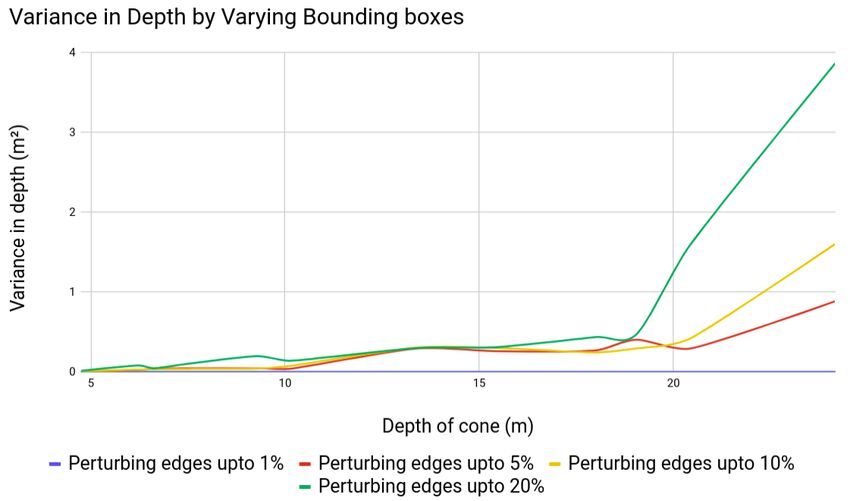
[13] C. Harris and M. Stephens. A combined corner and edge detector.
                                                                                    Citeseer, 1988.
                                                                               [14] K. He, X. Zhang, S. Ren, and J. Sun. Deep residual learning for image
                                                                                    recognition. In Proceedings of the IEEE conference on computer vision
                                                                                    and pattern recognition, pages 770–778, 2016.
                                                                               [15] S. Hecker, D. Dai, and L. Van Gool. End-to-end learning of driving
                                                                                    models with surround-view cameras and route planners. In European
                                                                                    Conference on Computer Vision (ECCV), 2018.
                                                                               [16] S. Hecker, D. Dai, and L. Van Gool. Learning accurate, comfortable
                                                                                    and human-like driving. In arXiv-1903.10995, 2019.
                                                                               [17] M. B. Jensen, M. P. Philipsen, A. Mgelmose, T. B. Moeslund, and
                                                                                    M. M. Trivedi. Vision for looking at traffic lights: Issues, survey, and
                                                                                    perspectives. IEEE Transactions on Intelligent Transportation Systems,
                                                                                    17(7):1800–1815, 2016.
                                                                               [18] W. Kehl, F. Manhardt, F. Tombari, S. Ilic, and N. Navab. Ssd-6d:
                                                                                    Making rgb-based 3d detection and 6d pose estimation great again. In
                                                                                    The IEEE International Conference on Computer Vision (ICCV), Oct
Fig. 11.     The variance observed in depth of cones when perturbing                2017.
the dimensions and position of bounding boxes that are input to the            [19] H. S. Lee and K. Kim. Simultaneous traffic sign detection and bound-
keypoint regressor. On the x-axis is the depth of the cone while the y-axis         ary estimation using convolutional neural network. IEEE Transactions
represents the variance in the cone’s depth estimate. Even with imprecise           on Intelligent Transportation Systems, 2018.
and inaccurate patches, the variance in depth estimates is quite low.          [20] J. Levinson, J. Askeland, S. Thrun, and et al. Towards fully
                                                                                    autonomous driving: Systems and algorithms. In IEEE Intelligent
                                                                                    Vehicles Symposium (IV), 2011.
                                                                               [21] J. Li, X. Liang, Y. Wei, T. Xu, J. Feng, and S. Yan. Perceptual
to estimate 3D pose from a monocular camera and by                                  generative adversarial networks for small object detection.
exploiting object structural priors. We demonstrate the                        [22] D. G. Lowe. Distinctive image features from scale-invariant keypoints.
                                                                                    International journal of computer vision, 60(2):91–110, 2004.
ability of the network to learn spatial arrangements of                        [23] M. Mathias, R. Timofte, R. Benenson, and L. V. Gool. Traffic sign
keypoints and perform robust regression even in challenging                         recognition how far are we from the solution? In International Joint
                                                                                    Conference on Neural Networks (IJCNN), 2013.
cases. To demonstrate the effectiveness and accuracy, the                      [24] R. McAllister, Y. Gal, A. Kendall, M. Van Der Wilk, A. Shah,
proposed pipeline is deployed on an autonomous race-car.                            R. Cipolla, and A. Weller. Concrete problems for autonomous vehicle
The proposed network runs in real-time with 3D position                             safety: Advantages of bayesian deep learning. In International Joint
                                                                                    Conference on Artificial Intelligence, 2017.
deviating by only 1m at a distance of 16m.                                     [25] J. Redmon, S. Divvala, R. Girshick, and A. Farhadi. You only look
                                                                                    once: Unified, real-time object detection. In Proceedings of the IEEE
                                                                                    conference on computer vision and pattern recognition, pages 779–
   Acknowledgement. We would like to thank AMZ Driver-                              788, 2016.
less for their support. The work is also supported by Toyota                   [26] J. Redmon and A. Farhadi. YOLO9000: better, faster, stronger. CoRR,
Motor Europe via the TRACE-Zurich project.                                          abs/1612.08242, 2016.
                                                                               [27] S. Ren, K. He, R. Girshick, and J. Sun. Faster r-cnn: Towards real-
                                                                                    time object detection with region proposal networks. In Advances in
                             R EFERENCES                                            neural information processing systems, pages 91–99, 2015.
                                                                               [28] O. Ronneberger, P. Fischer, and T. Brox. U-net: Convolutional
 [1] Cross ratio.     http://robotics.stanford.edu/˜birch/                          networks for biomedical image segmentation. CoRR, abs/1505.04597,
     projective/node10.html.                                                        2015.
 [2] OpenCV calibration and 3d reconstruction.                      https:     [29] A. Ruta, F. Porikli, S. Watanabe, and Y. Li. In-vehicle camera traffic
     //docs.opencv.org/2.4/modules/calib3d/doc/                                     sign detection and recognition. Machine Vision and Applications,
     camera_calibration_and_3d_reconstruction.html#                                 22(2):359–375, Mar 2011.
     solvepnp.                                                                 [30] C. Sakaridis, D. Dai, and L. Van Gool. Semantic foggy scene
 [3] PyTorch. https://pytorch.org/.                                                 understanding with synthetic data. International Journal of Computer
 [4] ROS: Robot Operating System. https://ros.org/.
 [5] H. Bay, T. Tuytelaars, and L. Van Gool. Surf: Speeded up robust                Vision, 2018.
                                                                               [31] S. Savarese and L. Fei-Fei. 3d generic object categorization, localiza-
     features. In European conference on computer vision, pages 404–417.
     Springer, 2006.                                                                tion and pose estimation. 2007.
 [6] D. Dai and L. Van Gool. Dark model adaptation: Semantic image             [32] R. Szeliski. Computer vision: algorithms and applications. Springer
     segmentation from daytime to nighttime. In IEEE International                  Science & Business Media, 2010.
                                                                               [33] S. Tulsiani and J. Malik. Viewpoints and keypoints. CoRR,
     Conference on Intelligent Transportation Systems, 2018.                        abs/1411.6067, 2014.
 [7] J. Deng, W. Dong, R. Socher, L.-J. Li, K. Li, and L. Fei-Fei. Imagenet:   [34] C. Urmson, J. Anhalt, H. Bae, J. A. D. Bagnell, and et al. Autonomous
     A large-scale hierarchical image database. In Computer Vision and              driving in urban environments: Boss and the urban challenge. Journal
     Pattern Recognition, 2009. CVPR 2009. IEEE Conference on, pages                of Field Robotics Special Issue on the 2007 DARPA Urban Challenge,
     248–255. Ieee, 2009.                                                           Part I, 25(8):425–466, June 2008.
 [8] A. Fregin, J. Mller, and K. Dietmayer. Three ways of using stereo         [35] A. Valada, J. Vertens, A. Dhall, and W. Burgard. Adapnet: Adap-
     vision for traffic light recognition. In IEEE Intelligent Vehicles             tive semantic segmentation in adverse environmental conditions. In
     Symposium (IV), 2017.                                                          Robotics and Automation (ICRA), 2017 IEEE International Conference
 [9] R. Girshick. Fast r-cnn. In Proceedings of the IEEE international
     conference on computer vision, pages 1440–1448, 2015.                          on, pages 4644–4651. IEEE, 2017.
                                                                               [36] P. Viola and M. Jones. Rapid object detection using a boosted cascade
[10] R. Girshick, J. Donahue, T. Darrell, and J. Malik. Rich feature
     hierarchies for accurate object detection and semantic segmentation.           of simple features. In Computer Vision and Pattern Recognition,
     In Proceedings of the IEEE conference on computer vision and pattern           2001. CVPR 2001. Proceedings of the 2001 IEEE Computer Society
                                                                                    Conference on, volume 1, pages I–I. IEEE, 2001.
     recognition, pages 580–587, 2014.                                         [37] Y. Xiang, T. Schmidt, V. Narayanan, and D. Fox. Posecnn: A
[11] G. Gkioxari, B. Hariharan, R. Girshick, and J. Malik. Using k-poselets
     for detecting people and localizing their keypoints. In Proceedings of         convolutional neural network for 6d object pose estimation in cluttered
                                                                                    scenes. CoRR, abs/1711.00199, 2017.
     the IEEE Conference on Computer Vision and Pattern Recognition,           [38] Z. Zhu, D. Liang, S. Zhang, X. Huang, B. Li, and S. Hu. Traffic-sign
     pages 3582–3589, 2014.                                                         detection and classification in the wild. In Proceedings of the IEEE
[12] D. Glasner, M. Galun, S. Alpert, R. Basri, and G. Shakhnarovich.
     aware object detection and continuous pose estimation. Image and               Conference on Computer Vision and Pattern Recognition, 2016.
     Vision Computing, 30(12):923–933, 2012.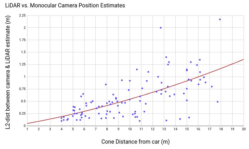
You can also read