Proofreading Tile Sets: Error Correction for Algorithmic Self-Assembly
←
→
Page content transcription
If your browser does not render page correctly, please read the page content below
Proofreading Tile Sets:
 Error Correction for Algorithmic Self-Assembly

                        Erik Winfree and Renat Bekbolatov

               Computer Science and Computation & Neural Systems
           California Institute of Technology, Pasadena, CA 911125, USA

       Abstract. For robust molecular implementation of tile-based algorith-
       mic self-assembly, methods for reducing errors must be developed. Pre-
       vious studies suggested that by control of physical conditions, such as
       temperature and the concentration of tiles, errors (ε) can be reduced
       to an arbitrarily low rate – but at the cost of reduced speed (r) for
       the self-assembly process. For tile sets directly implementing blocked
       cellular automata, it was shown that r ≈ βε2 was optimal. Here, we
       show that an improved construction, which we refer to as proofreading
       tile sets, can in principle exploit the cooperativity of tile assembly reac-
       tions to dramatically improve the scaling behavior to r ≈ βε and better.
       This suggests that existing DNA-based molecular tile approaches may be
       improved to produce macroscopic algorithmic crystals with few errors.
       Generalizations and limitations of the proofreading tile set construction
       are discussed.

1    Introduction

The experimental demonstration that DNA can be used to encode and process
information [1] has stimulated interest in how biomolecular processes can be
programmed to carry out logical algorithms. Algorithmic self-assembly of DNA
tiles has been proposed as the basis for parallel computation of solutions to
hard combinatorial problems [27, 30, 18, 12] and for bottom-up nanofabrication
of complex structures that can be specified by simple rules [23, 20, 8].
    Understanding of this approach relies upon an abstract model of the growth
process, known as the abstract Tile Assembly Model (aTAM). As in Wang’s
Tiling Problem [25, 26], a tile system consists of a finite set of square tiles with a
label on each side. For simplicity, tiles cannot be rotated. The aTAM augments
these tiles with a strength function that specifies how tightly tiles stick to each
other when the labels on touching sides match (referred to as a bond). This
motivates a growth rule: starting with a specified seed tile, a new tile may be
added at any position where the total strength of all newly-formed bonds exceeds
a threshold, τ . This rule is intrinsically asynchronous and non-deterministic:
only certain tile sets will produce a uniquely-defined structure. The aTAM is
illustrated in figure 1ab, using a tile set we call the Sierpinski tiles; at τ = 2, the
growth results [28] in an infinite Sierpinski triangle pattern [5].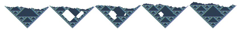
(a)              rule tiles              boundary tiles                      seed tile
 output                                                                                   strength−2 (strong) bond
  input                                                                           strength−1 (weak) bond
        0+0=0 0+1=1 1+0=1 1+1=0                                           strength−0 (null) bond

 (b)                                      (c)

                                                     rf      r r,2
                                                                     rf   r r,1   rf
                                                                                       r r,1   rf
                                                                                                    r r,2

         τ =2                                   rf
                                                          r r,0                           rf
                                                                                  r r,5

Fig. 1. (a) The seven Sierpinski tiles include four rule tiles implementing the XOR
logic and three boundary tiles, including the corner tile which is used as the seed tile.
Whereas all sides of the rule tiles form strength-1 (weak) bonds, the boundary tiles also
make use of strength-2 (strong) bonds and strength-0 (null) bonds. Strong bonds are
drawn as double lines, and null bonds are drawn as thick lines. This construction can
be trivially generalized to implement an arbitrary BCA with more than two symbols.
(b) Growth of the Sierpinski tiles from the seed tile according to the aTAM at τ = 2.
The small tiles indicate the (only) four sites where growth can occur. At each location,
there is a unique tile that may be added, and a unique pattern results. (c) Rates for tile
addition and tile dissociation in the kTAM: rf is the forward rate for association of any
tile at any site, and rr,b is the reverse rate for dissociation of a tile that makes bonds
with total strength b. All and only single monomer tile associations and dissociation
events are considered in the kTAM; a representative selection is shown here.

    The Sierpinski rule tiles implement a replacement rule (x, y) → (z, z) where
x, y ∈ {0, 1} and z = (x + y) mod 2; each tile has some x and some y on the
bottom two sides and the corresponding z on both top sides. This is an instance
of a one-dimensional blocked cellular automaton (BCA): an initial string, the
bottom layer, is transformed for each subsequent layer by partitioning the string
into pairs (alternately odd/even-indexed and even/odd-indexed elements) and
replacing each pair according to a rule (x, y) → (f1 (x, y), f2 (x, y)), where all
values are in an alphabet, e.g., {0, 1, . . . , N }. Generalizing the Sierpinski rule
tiles to rule tiles whose inputs and outputs may take on (N + 1) values yields
a direct implementation for any chosen BCA: one rule tile is used for each of
(N + 1)2 possible input pairs, and the initial conditions for the computation
are given using boundary tiles with strength-2 bonds that grow from the seed
tile. We call this the direct tile set for a given BCA. Since BCA are capable of
Turing-universal computation, this implies that tile-based self-assembly provides
a natural logical basis for programmable self-assembly processes with arbitrary
complexity. We now need to find a physical process, such as DNA tile assembly,
wherein self-assembly occurs (at least approximately) according to the aTAM
rules at τ = 2, using tiles with bond strengths restricted to 0, 1, and 2.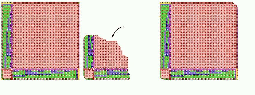
Tile-based self-assembly of two-dimensional periodic structures has been suc-
cessfully demonstrated experimentally using a variety of molecular implementa-
tions of DNA tiles [29, 11, 14, 31]. The key principle is that each DNA molecule
has four short single-stranded regions, known as sticky ends, which direct how
the DNA tiles bind to each other: sticky ends with complementary sequences can
form a thermodynamically favorable double-helix, as shown in figure 2 for DNA
tiles made from DNA double-crossover molecules [9]. Attempts at algorithmic
self-assembly in one dimension [13] and in two dimensions [19] have also proven
successful, but with two limitations: (1) incorrect tiles are incorporated into the
growing structure with error rates ranging from 1% to 10%, and (2) spurious
nucleation (not involving the seed tile) results in many structures that perform
the wrong computation and thus produce an undesired structure.
    Our concern in this paper is how to control growth errors.1 We can consider
four approaches to reducing growth errors.

Logical error correction. Accept an intrinsic error rate ε, and design a larger
   tile set that contains logic to detect and correct errors. In principle, this
   should be possible by making use of one-dimensional fault-tolerant cellular
   automata [10], but it is likely to be extremely complicated.
Optimized physical conditions. Study how physical conditions, such as tem-
   perature, tile concentrations, and buffer conditions, determine the error rate,
   and optimize them to obtain the best performance. As was shown in [28],
   this approach is promising, but it is likely to require extremely slow growth
   conditions.
New molecular mechanisms. Devise new physical mechanisms, such as, for
   example, more complicated molecular implementation of tiles with latches
   and switches. However, new structural motifs are difficult to design and
   characterize, so this approach must be considered with caution.
Exploiting cooperative binding. While retaining the original molecular tile
   design, redesign the original tile set to exploit physical mechanisms already
   inherent in the self-assembly process. This combined approach, which relies
   both on logical aspects of the tile set and on physical aspects of the assembly
   process, is explored here with dramatic benefits.

2     The kinetic Tile Assembly Model: error vs growth rates

Both growth errors and nucleation errors can be understood in terms of an ex-
tension of the aTAM to include rates both for tiles associating to and for tiles
dissociating from the growing crystal (figure 1c); this model is known as the
kinetic Tile Assembly Model (kTAM) [28]. The on-rates and off-rates can be
chosen according to the principles of DNA hybridization [4], as illustrated in
figure 2 for tiles implemented as DNA double-crossover (DX) molecules [9]. The
fundamental observation is that while on-rates depend only upon the concentra-
tion of the tiles, the off-rates depend exponentially upon the total strength of
1
    Nucleation errors will be treated in an upcoming paper [22].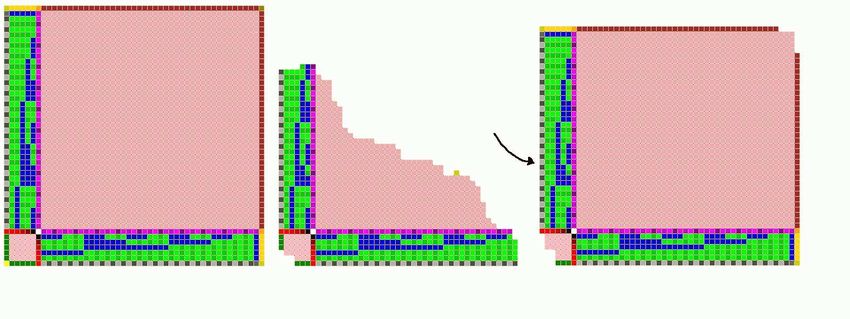
(a)
     TCACT                 CATAC

                                      AGAAC              ATCTC

     TAGAG                 TCTTG

                                      GTATG              AGTGA
                                                                      kf   k r,1
                            kf     k r,1

 (b)

                                 kf     k r,2                                kf    k r,2

Fig. 2. (a) Assembly of two double-crossover tiles via hybridization of 5-nucleotide
sticky ends. kf is the forward rate constant, in /M/sec, and kr,1 = kf e−Gse is the
reverse rate constant, in /sec. (b) Assembly of a double-crossover tile into a site on
the growth front of a crystal via hybridization of two 5-nucleotide sticky-end pairs. The
forward rate constant is assumed to be the same as for the single sticky-end reaction
of (a), while the reverse rate constant is assumed to require twice as much energy to
simultaneously break both sticky-end bonds – i.e., binding is cooperative – and thus
kr,2 = kf e−2Gse . Gse is the free energy of dissociation for a single sticky end, in units
of RT .

molecular interactions, i.e., the number of base pairs that must be broken in or-
der for the tile to dissociate. Thus, single tiles (monomers) that either totally or
partially mismatch their neighbors arrive at a site with equal frequency as tiles
that correctly match their neighbors, but the correctly-matching tiles stay much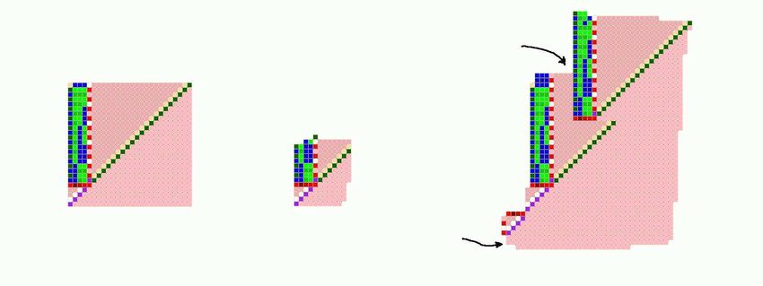
longer. These considerations suggest that behavior of the system is character-
ized by two essential physical parameters, Gmc and Gse , respectively measuring
the monomer concentration and the sticky-end bond strength as unitless free
energies. Specifically, we define [monomer tile]/M = e−Gmc , and thus Gmc is
primarily entropic, as it measures the spatial degrees of freedom that are lost
when a free-floating monomer tile is localized on the assembly.2 Similarly, we
define the free energy of dissociation of a single sticky end to be ∆G/RT = G se ,
and thus Gse contains a mix of entropic and enthalpic factors related to the
formation of the double-helix, measured in units of RT .
    We can now formulate the kTAM to describe the growth of a single crys-
tal in an environment where the concentration of monomer tiles remains fixed.
Absolute rates for events affecting this crystal are given by

                           rf = kf [monomer tile] = kf e−Gmc

for association of a new monomer tile at any given site, and

                                  rr,b = kr,b = kf e−bGse

for dissociation of a tile whose interactions with the crystal sum to b, in the
“strength units” of the aTAM. b can be thought of as the effective number of
unit-strength sticky ends binding the tile to the crystal. These rates specify a
continuous-time Markov process (satisfying detailed balance) for modeling the
growth of a single crystal in a solution of free monomer tiles.3
2
    The simplest situation is when all monomer tile species are present at the same con-
    centration of each species. In some cases, it is convenient to specify the stoichiom-
    etry of the tile species, relative to the “generic” monomer tile whose concentration
    is determined directly by Gmc . For example, in the Sierpinski tile simulations, the
    boundary tiles are present at half the concentration of the rule tiles, which ensures
    that the boundary grows at approximately the same speed as the interior.
3
    Our model assumes that only single tiles associate to and dissociate from an as-
    sembly. Solution will contain a distribution of assembly types, from dimers (two
    tiles bound to each other) on up. However, near the melting temperature for crys-
    tals, where our results hold, dimer concentrations should be significantly lower than
    monomer concentrations, and thus dimer association events should be rare. Likewise,
    a pair of connected tiles may simultaneously dissociate from an assembly, or assem-
    blies can even fracture into two or more large pieces. However, the energy required
    for such events is typically significantly greater than that for monomer dissociation.
    Therefore, we do not expect our results to change qualitatively if evaluated under
    more sophisticated models. For the tile sets discussed here, we have seen only minor
    quantitative changes when either (a) the model also allows tile dissociation events
    wherein after removal of the tile, the assembly falls apart into two unconnected pieces
    (such reactions are not reversible in the context of a single-crystal model, and thus
    are excluded from the standard kTAM), or (b) additionally, the model allows dimers
    or 2x2 blocks to dissociate together. There are tile sets for which these modification
    do have qualitatively significant ramifications, for example, tile sets involving linear
    polymerization or blocks of tiles that are strongly bound to each other but have
    weak interactions with the crystal.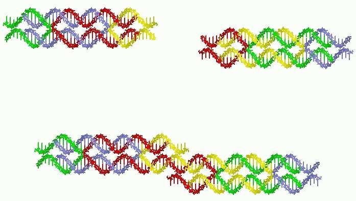
optimal
                               growth constant ε

   low               τ=2                            (a)                                  (b)

                                      ls
                                   ta
                                 ys
[monomer]

                               cr
             no growth

                           od
                                           τ=1

                          go
                                                                                               FC             FM
                                                          r*                        r*
    G mc                                                                                           r*               r*
                                                                                               C              M

                                                                        rr,                            r f rr,1 r
                                     fast                          rf      1   rf              r r,2            f
                                   random                  r r,2
                                 aggregation                                                             E
  high
[monomer]

            weak                           strong
            bonds          G se            bonds
            (hot)                          (cold)

                         (a)                                                  (b)
Fig. 3. (a) Phase diagram [28] for crystal growth of tiles implementing a BCA, under
the kTAM. “Good crystals” (growth rate comparable to kf [DX] and error rate smaller
than ε) are obtained for large Gse and Gmc , below the τ = 2 boundary marking the
melting transition where Gmc = 2Gse . (b) Model for kinetic trapping. The growth site
may (E) be empty; (C) contain a correct tile; (M ) contain a mismatched tile; (F C) be
“frozen” with the correct tile in place; or (F M ) be “frozen” with the mismatched tile.
r∗ represents the rate at which tiles on the growth front are covered. The error rate is
taken to be the probability that, starting in E, the system reaches F M .

    The parameters Gmc and Gse represent the “physical conditions” under
which tile-based assembly can take place. Gmc can be made large (or small)
by using DNA tiles at low (or high) concentrations. Gse can be made large (or
small) by letting the self-assembly take place at a cold (or hot) temperature. 4
For what settings of these parameters does the kTAM obey the aTAM rules with
high probability? First note that if 2Gse > Gmc > Gse , then the tile additions
shown in figure 1b are favorable, as rf > rr,2 , but all other tile additions are un-
favorable, as they make at most 1 bond and rf < rr,1 . Thus, the aTAM correctly
abstracts which reactions are favorable, and which are unfavorable, with respect
to the kTAM. However, in the kTAM, unfavorable reactions also occur with some
frequency, so we expect assembly errors. Figure 4a shows several snapshots from
a Monte Carlo stochastic simulation; single growth errors occur in the 3 rd and
4th frames, causing subsequent error-free growth to develop into an undesired
pattern. How frequent are these errors, and how can they be minimized?

4
    Naturally, the assumption that Gmc and Gse both remain constant is likely to be
    violated in actual experiments, both for reasons under our control (e.g., using a
    temperature annealing schedule) and for reasons not easily under our control (e.g.,
    the depletion of ambient monomer tile concentrations as a significant fraction of tiles
    become incorporated into crystal assemblies.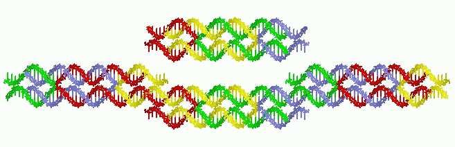
Previous studies [28] using this model showed that both growth errors and
certain nucleation errors5 can be controlled in the limit of low monomer tile
concentrations (i.e., large Gmc ) and strong sticky-end interactions (i.e., large
Gse ) so long as the system is kept near the melting temperature of the crystal
(i.e., Gmc ≈ 2Gse ). As shown in figure 3a, phase space can be divided into
three regions: no crystal growth occurs if Gmc > 2Gse ; algorithmic self-assembly
(with some error rate) occurs for 2Gse > Gmc > Gse ; and essentially random
aggregation is obtained for Gse > Gmc . Within the algorithmic phase, two factors
limit the performance that can be achieved: thermodynamics tells us the best
error rate that can be achieved at equilibrium given the energetics of the system,
while the kinetics determine how quickly we get there – if at all.
    If self-assembly achieves equilibrium, the probability of observing a particular
assembly A will be governed by the Boltzman equation:

                                1 −G(A)                  X          0
                     P r(A) =     e         with    Z=         e−G(A )
                                Z
                                                          A0

where G(A) = nGmc − bGse is the free energy of the assembly, n is the number
of tiles in the assembly, b is the total of all bond strengths in the assembly, and
Z is the partition function. Thus, an n-tile assembly that has ∆b more bond
strength than another n-tile assembly will be e∆bGse more likely. In a direct
BCA tile set with (N + 1) states, a typical growth site will present two sides
with strength-1 bonds, a unique correct tile will match both bonds, and there
will be exactly N competing tiles that have a mismatch on the left side, as well
as N that have a mismatch on the right side. It follows that the equilibrium
probability of incorporating the correct tile at a given growth site is

                                e2Gse
                  1−ε≈                     , and thus ε ≈ 2N e−Gse ,
                           e2Gse + 2N eGse
where ε is the per-tile error rate. It is mildly surprising that Gmc has no effect
on the equilibrium error rates.
    However, due to kinetics, equilibrium is seldom achieved far below the melting
transition. The primary cause of growth errors in this case was found to be a form
of kinetic trapping, wherein tiles that associate with a mismatch on the growth
front don’t have time to dissociate, and are frozen in place by further growth;
thus equilibrium error rates are observed only near the melting transition. The
essential feature of kinetic trapping within BCA tile self-assembly is that once
an error has occurred, both sites above the mismatched tile display an (x, y)
pair that is perfectly matched by some monomer tile in solution, because tiles
implementing all replacement rules (x, y) → (f1 (x, y), f2 (x, y)) are present. Thus,
5
    It was shown that spurious nucleation of rule tiles can be controlled, for essentially
    the same reason that supersaturated solutions can be maintained: there is a critical
    nucleus size (based on surface-to-volume energies) beyond which growth is favorable
    and below which growth is unfavorable. However, spurious nucleation of boundaries
    is a more difficult issue [21].
(a)
(b)
(c)
Fig. 4. (a) Growth of the original (1 × 1) Sierpinski tile set at Gmc = 13.9 and Gse =
7.0, to a size of ∼ 32 layers in ∼ 530 simulated seconds. Two errors can be seen; the first
occurs in the third frame and is indicated by an arrow. Subsequent error-free growth
correctly propagates the erroneous information. (b) Growth of the 2 × 2 proofreading
tiles at Gmc = 12.9 and Gse = 6.5, to a size of ∼ 64 layers in ∼ 460 simulated seconds.
(c) Growth of the 3 × 3 proofreading tiles at Gmc = 11.9 and Gse = 6.0, to a size of
∼ 96 layers in ∼ 310 simulated seconds.
if such a tile arrives before the mismatched tile dissociates, the mismatched tile
becomes locked in by multiple bonds, and is now unlikely to dissociate. For a
direct BCA tile set, the kinetic trap model shown in figure 3b accurately predicts
growth errors in kTAM simulations to obey [28]
1 r∗ + rr,2
1−ε≈ r ∗ +rr,2 and thus ε ≈ 2N −→ 2N e−Gse ,
1 + 2N r ∗ +rr,1
r∗ + rr,1 r ∗ →0
where r = 21 (rf − rr,2 ) is the overall growth rate and r ∗ = αr is the effective rate
at which sites are frozen in the model. α = 1.5 is a free parameter chosen fit to
the data; in some sense, it accounts for the fluctuations of the growth process, in
which the growth front will wash back and forth over a given site several times
before it is “frozen” in place.
The kinetic trapping theory identified a critical relationship. Although arbi-
trarily low error rates can be achieved by appropriate choice of Gmc and Gse ,
they come at the cost of a significant slow-down. This trade-off can be visual-
ized by plotting r vs ε for all reasonable values of Gmc and Gse . As illustrated
by the upper (1 × 1) plots in figure 5, all points lie above r ≈ βε2 , whereSimulation and Kinetic Trap Predictions for Proofreading Tiles
−2
10
1x1 slope=0.49963
error rate (mismatches/tile)
−3
10
2x2 slope=1.0325
−4
10
−5
10
3x3 slope=1.1277
−6
10
−7
10
−4 −3 −2 −1 0 1
10 10 10 10 10 10
speed (layers/sec)
Fig. 5. Plot of error rate vs. growth speed as measured in simulations (*’s) and as
according to kinetic trap theory (lines). Here, Gmc = 2 ∗ Gse − ; i.e., measures how
far the reaction is from the τ = 2 melting transition. Curved lines (red and blue) vary
Gmc and for fixed Gse , thus demonstrating how the growth speed decreases too near
the melting transition and the error rates increases too far below the melting transition.
(Simulations used Gse = 6.5 and 8.5 for 1 × 1, 6.5 and 7.5 for 2 × 2, and 5.5 and 6.5
for 3 × 3 tile sets.) Straight lines (green) vary Gse and Gmc for fixed , thus following
the line just below the melting transition in phase space to obtain a Pareto-optimal
speed/error trade-off. (Simulations used kf = 106 /M/sec and = .2, .1, .15 for 1 × 1,
2×2, and 3×3 tile sets respectively. Error bars show two standard deviations, computed
√ √
using σ = ε/ m where m is the total number of tiles grown in all simulations using
a given Gse and Gmc . A variable number of simulation runs were used, chosen to make
the error bars small. )
β ≈ 1 × 10⁴ /M/sec is determined by how far below the melting temperature
gives the optimal trade-off.6 This defines the Pareto-optimal boundary along
which r is the fastest growth rate that achieves error rate ε. Thus, decreasing
error rates by a factor of 10 entails slowing down the self-assembly process by
a factor of 100. This is bad; results on fault-tolerant computing in the digital
k
6
If Gmc = 2Gse −, then r = 12 (rf −rr,2 ) = 21 kf (e −1)e−2Gse ≈ 8Nf2 ε2 for equilibrium
error rates. This estimate is accurate only within an order of magnitude.circuit model typically entail a logarithmic, rather than quadratic, slow-down
[24, 15].
In the rest of the paper, we give a construction of “proofreading” tile sets to
implement arbitrary BCA, in which each original tile is replaced by a K × K
block of tiles in the new tile set.7 Simulation and theory results for 2 × 2 and
3 × 3 tile sets are shown in figures 4 and 5, showing scaling behavior of roughly
r ≈ βε1.0 and r ≈ βε0.89 respectively, with β varying by less than a factor of
five depending on the tile set. This is a significant improvement: for target error
rates of 10−4 , the 2 × 2 proofreading tiles result in a 104 -fold speed-up over the
original tile set. Similarly, for the same physical conditions that result in a 1%
error rate for the original tile set, the 2 × 2 proofreading tile set yields a 0.01%
error rate, and the 3 × 3 proofreading tile set yields a 0.001% error rate. This
is extremely encouraging for experimental studies of algorithmic self-assembly:
conditions in which perfect 10 × 10 Sierpinski triangles can now be grown may
yield 100 × 100 triangles with proofreading tiles. Still, these constructions result
in greater slow-down than achieved in the digital circuit model, suggesting that
further improvements await discovery.
The remainder of this paper describes the proofreading tile set construction,
gives an explanation of the principles by which it works, and comments on its
limitations.
3 Proofreading tile sets
The ability for the kTAM to discriminate between tiles that partially or perfectly
match a growth site relies on the cooperativity of sticky-end binding: the binding
of one sticky end stabilizes the binding of the other sticky end. The basic idea
of proofreading tiles is to exploit cooperative binding at the next higher level:
to have several tiles that stabilize each other when they bind together. Cooper-
ative binding is a common feature of transcription factors in genetic regulatory
networks [16] and has been examined as a mechanism for increased sensitivity
in one-dimensional self-assembly processes [2, 3]. New issues arise in the context
of two-dimensional self-assembly.
The general 2 × 2 proofreading construction is shown in figure 6a, and its
application to the Sierpinski tile set is shown in figure 6bcd. Essentially, each rule
tile in the original tile set is replaced by four tiles with related labels. Arranged
in a 2 × 2 block, the sides of the block present the same logical labels as the
original tile. The side internal to the block are given unique labels, not shared
by tiles from any other block. Thus, assembly from the seed tile according to the
aTAM proceeds according to the same logic as the original tile set, but scaled
up in size by a factor of two.8 However, in the kTAM, a new phenomenon can be
observed when a mismatched tile is incorporated: there is now no way to continue
7
The direct BCA tile sets can be considered to be the 1×1 proofreading construction.
8
For self-similar patterns like the Sierpinski triangle, the resolution of the resulting
pattern remains the same – each 2 × 2 block can be labeled according to the pre-
computed pattern.(a)
c’
d’
x3
x4
2x2 block X
tile X
x3
x4
c
c
d
d
(4 tiles)
b’
x1
x2
b
a
a’
x1
x2
b
a
rule tiles boundary tiles
(b)
0+0=0 0+1=1 1+0=1 1+1=0
(c)
(d)
Fig. 6. (a) The general 2 × 2 proofreading construction for rule tiles. (b) The original
Sierpinski tiles. (c) The 2×2 proofreading Sierpinski tiles. (d) Growth of the proofread-
ing Sierpinski tiles. Small tiles illustrate that when a mismatched tile is incorporated,
further growth on one side must involve a second mismatch.
growth without making an additional error. This is illustrated by the small tiles
in figure 6d: after the initial (lowest) small tile arrives, forming a mismatch
on one side, any further tile assembling on that side will either (a) agree with
the initial tile but, because it therefore must be part of the same proofreading
block, mismatch on its lower right side, or (b) agree with its lower right input,
but therefore form a mismatch with the initial small tile. The assembly process
stalls, giving time for the initial mismatched tile to fall off and be replaced by
a correct tile. The final assembly therefore has no record of the mishap having
occurred.(a) FM FC
r* r*
rr,4
rr,3 rr,3 rr,1 rr,1
rr,1
rr,2 rr,2 rr,2 rr,1 rr,2 rr,1 2rr,3
rr,2
rf rf 2Nrf
rf rf
rf rf rf rf rf rf rf rf rf
rr,1 rr,1 rr,1 rr,1 rr,2 rr,2 2rr,2
rr,1 rr,2 rr,1 rr,1
rr,2 rr,1 rr,1 rr,3 2rr,2
rf
Nrf rf rf rf rf rf
rf rf rf Nrf rf
rf rf rf rf
rr,2 rr,2
rr,1 rr,2 rr,2 rr,1 rr,1 rr,3 rr,1
rf 2Nrf 2rf
rf rf rf rf rf rf
rr,1 rr,1 rr,2 rr,1
2Nrf rf
2Nrf 2rf
(b)
r* rf 2rf rf 4Nrf rf 2rf rf rf r*
FC M4 M3 M2 M1 E C1 C2 C3 C4 FC
2rr,2 rr,1 2rr,2 rr,1 rr,2 rr,2 2rr,2 rr,2
Fig. 7. (a) A kinetic trapping model including all 29 states (up to symmetry) repre-
senting “well-associated” tiles within a 2 × 2 growth site (see text for details). Arrows
inside tiles indicate that the tile belongs to a proofreading block that has a mismatch
to the input in the indicated direction; there are N such tiles for an (N + 1)-state
BCA. Arrows between states indicate reversible reactions (association or dissociation
of a tile); reverse reaction rates are given at the head of each arrow, and forward reac-
tion rates are given near the tail. States within dotted circles each have an irreversible
reaction to a frozen state (either FM or FC) with rate r ∗ . (b) A simplified kinetic
trapping model with 9 states considers only the major reaction pathways in (a), which
are indicated by the red and green reaction arrows for pathways leading to mismatched
or correct blocks, respectively.
The forcing of errors to be co-localized in pairs results in the error rate being
squared relative to the original tile set. A detailed kinetic trapping model for
2 × 2 proofreading tiles (shown in figure 7a) produces excellent agreement 9 with
the simulation results (shown in figure 5), including the precipitous decline in
reliability as physical conditions move away from the melting transition. Each
state in this model represents a possible arrangement of tiles (up to symmetries)
within the 2 × 2 growth site. Each tile could be either part of the correct block
for that site (unlabeled) or part of a block that has a mismatch on one side
or the other (indicated by the direction of the arrow; there are N such blocks
9
Again, the value of r ∗ was determined by fitting free parameters to best match the
data. Here, we used r ∗ = αreγ where = 2Gse − Gmc , α = 1, and γ = 12. We have
no strong justification for this formula.for BCA tile sets). The 29 states considered are all those in which the tiles are
“well-associated”, that is, we prune the full model by removing all states in
which more than one tile is attached by only one bond or in which some tile is
attached by no bonds at all – such states would be very short-lived.
A simplified model (shown in figure 7b) considers just the dominant path-
ways (red and green reaction arrows in figure 7a), and yields similar results near
the melting transition. The improvement in the error rate near the melting tran-
sition, then, is due to the elementary features preserved in this model, namely
that (a) the correct block can be formed via a series of four favorable steps,
and (b) every path to a mismatch contains at least two significantly unfavorable
steps with a fast rr,1 reverse reaction.
Although baroque, both models can easily be solved numerically by repre-
senting the transition rates in matrix form and computing the steady-state by
matrix inverse.
The basic phenomenon can be more easily understood using the following in-
tuition. Consider first the direct BCA tile set. Optimal growth rates are obtained
near the melting temperature of the crystals, where Gmc ≈ 2Gse . Under these
conditions, the error rate reaches the thermodynamic limit of ε ≈ e−∆G/RT =
e−Gse , where ∆G is the difference in free energy between an assembly with a
mismatched tile and one with a correct tile. However, the growth rate will be
proportional to the monomer tile concentration, r ≈ β[DX] = βeGmc . This
yields the scaling relation for the original tile set, r ≈ βε2 .
This type of argument can be generalized for K × K proofreading construc-
tions, wherein each tile is replaced by a K × K block of unique tiles. Optimal
growth rates still occur near the melting temperature (Gmc ≈ 2Gse ), and the
growth rate is still r ≈ β[DX] = βeGmc . However, the thermodynamic error rate
(for an entire block) is now determined by the minimal error, which involves at
least K mismatched tiles.10 Thus11 ε ≈ e−∆G/RT = e−KGse , and the argument
yields r ≈ βε2/K .
If the above reasoning held for all K, and the proofreading block size were
to be chosen based on the target error rate needed, a logarithmic dependence of
K on the target error rate would be achieved for constant physical conditions.
This matches what has been found for digital circuits. Unfortunately, although
the argument correctly predicts the scaling behavior for K = 2, the simulation
results for K = 3 (figure 5) and K = 4 (data not shown) fall short of the
prediction.
We attribute this failure to a second mechanism for growth errors. Whereas
proofreading tiles perform well at correcting errors during growth at a site where
10
Since each erroneous block involves K 2 tiles and typically contains exactly K mis-
matches, the per-block error rates εblock = Kε, where ε is the per-tile error fraction.
(Tile errors are now clearly not iid.) We found it more convenient to report simula-
tion results in terms of the per-tile error rate.
11
This argument illustrates why it is necessary to use cooperativity by relying on
the independent assembly of the K 2 pieces in a block. If one were to use a pre-
assembled block, the melting temperature would occur at Gmc ≈ 2KGse , giving rise
to the original r ≈ βε2 scaling behavior.correct growth could occur, they do nothing to prevent errors due to spontaneous
growth on a facet (“roughening”), as shown in figure 8a. Ensuring that bound-
aries grow at approximately the same speed as the interior12 reduces the amount
of faceting, but even so, facets of length n appear with a frequency of ≈ 2 −n ,
making facet growth errors rare but unavoidable. Some other error-correcting
strategy will be necessary to prevent this type of error.
4 Strong bonds, capping tiles, and self-repair
It is important to realize that the proofreading tile set construction given here
doesn’t work for all tile sets. The existence of the alternative growth error mech-
anism on facets implies that tile sets whose growth process intrinsically involves
facets will fail to derive great benefit from proofreading tiles. For example, the
the tile set presented in [20] for growing M × M squares using O(log M ) tiles
results in a final assembly in which three sides are facets – i.e., each tile on those
sides displays a strength-1 bond, but under τ = 2 aTAM rules, no growth can
occur. In the kTAM, growth will eventually occur, ruining the desired structure,
as shown in figure 8b(top) for a 26 × 26 square. Proofreading tiles do nothing to
fix this problem.
To reliably construct an M × M square required modifying the original tile
set in three ways: first, identifying the direction of growth and specializing the
tiles so that each tile is used for only one direction of growth, and each sticky end
appears on as few tiles as possible; second, making use of additional “capping”
tiles to quickly cover the final facets of the square with tiles that have null bonds
on their outer sides, thus reducing errors due to roughening; and third, using
two perpendicular binary counters to encourage the growth front to avoid large
facets. Assembly using this improved tile set is shown in figure 8b(middle) for a
49 × 49 square.
With facet roughening errors ameliorated, it makes sense to ask whether now
proofreading further decreases the error rate. However, because growth of the
square within the counter region takes a meandering path making use of several
rule tiles with strength-2 bonds, the proofreading construction must be extended
to blocks involving strength-2 bonds. This construction, shown in figure 8c, can
only be used for tile sets in which each tile occurs only during growth in a
particular direction; i.e., its input and output sides can be determined and are
used consistently. The bond labels on proofreading tiles are as described previ-
ously, but the strength of those bonds is determined by the growth direction (for
the input sides) or by the growth direction of subsequent tiles (for the output
sides). This 2 × 2 proofreading construction was applied to the improved tile set
described above, with results shown in figure 8b(bottom).
Out of 31 trials, the original tile set never formed the desired 26 × 26 squares
properly, the improved tile set was 65% successful at forming 49 × 49 squares,
12
This is the case in the simulations, thanks to the boundary tile concentration being
set to 21 the concentration of the rule tiles.aTAM (early) kTAM (later)
original
improved
proofreading
(a) (b)
? ? ? ? ? ?
1 1 1 ? ? 1 1 ? ? S 2 2 ?
? ? ?
1 1 1 2 2 1
1 ? ? ? ? S ?
1 1 1 2 2 1
1 2 ?
1 1 1 ? ? 1 1 ? ? 1 1 ?
(c) 1 1 2 1 ? ?
Fig. 8. (a) Small black tiles illustrate spurious nucleation of the subsequent layer
(facet roughening). The information content of these tiles is likely to be wrong. Our
proofreading tile set construction does not efficiently correct these errors. (b) From
left to right: Assembly according to the aTAM at τ = 2; early growth in the kTAM
at Gmc = 17.7 and Gse = 9.0; and the resulting structure. From top to bottom:
The binary counter construction for assembling M × M squares; the improved two-
counter construction with capping tiles; and the 2 × 2 proofreading construction for
the latter. All tile sets assemble perfectly under the aTAM. Under the kTAM, the
one-counter tile set fails even for a small square because spurious nucleation on facets
frequently results in uncontrolled growth (arrows). The two-counter tile set still suffers
from algorithmic errors (arrow), but the capping tiles significantly reduce spurious
nucleation of new layers. The proofreading construction reduces these problems only
somewhat for this tile set. The arrow indicates a facet roughening error in which capping
tiles prematurely nucleated on the growth front. In this run, these capping tiles are
eventually displaced by the growth of correct tiles. (c) The scheme for assigning bond
strengths for proofreading tiles when the tile set contains strength-2 bonds. Arrows
indicate the direction of growth for correct use of the tile, and “S” indicates the seed
tile. The strength of bonds on sides marked by “?” is dictated by the tiles that bind to
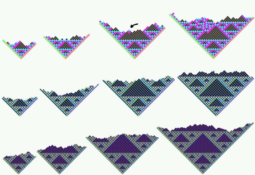
them in a correct assembly; if no tiles bind to them, strength-0 bonds are used.time
damage
scar
Fig. 9. Proofreading tile sets are often able to heal a puncture in the crystal. Sometimes,
as in this case, some of the tiles that fill in the puncture do not perfectly match their
neighbors – a form of “scar tissue.”
and the proofreading tile set formed 98 × 98 squares 87% of the time. For com-
parison, the improved tile set formed 99 × 99 squares only 26% of the time. The
disappointingly modest13 benefit provided by the proofreading tiles suggests that
alternative error mechanisms are dominant for these tile sets.
The proofreading tiles also give rise to some surprising, and pleasant, behav-
iors. One such phenomenon is their ability to heal punctures of the growing crys-
tal, as shown in figure 9. Since the identity of tiles within the punctured region is
uniquely determined by the perimeter of that region (in fact, just the lower por-
tion of the perimeter suffices), one might expect even the non-proofreading tile
set to be able to correctly fill in the punctured region. However, regrowth into the
punctured region may occur in any direction, including backward from the most
advanced edge of the puncture, where there are multiple ways to proceed locally
when using tiles implementing irreversible BCA, such as the Sierpinski tiles. 14
Thus, regrowth is not always perfect; indeed, the direct BCA tiles very often
leave “scar tissue”, although the proofreading tiles do so much less frequently.
5 Discussion
The primary result of this paper is that dramatic improvements in the error rates
for algorithmic self-assembly can be achieved, in principle, by proper redesign of
the abstract tile set, without changing the fundamental molecular implementa-
tion. The 2×2 proofreading tiles for BCA increase the optimal growth speed r for
which a target error rate can be achieved from r = β2 to r = β, and greater
improvements can be obtained with larger K × K proofreading constructions.
If these constructions hold up in practice, it may be possible for algorithmic
self-assembly to scale up to macroscopic assemblies without errors.
Although the theoretical and simulation results presented here firmly estab-
lish the effectiveness of the proofreading tile construction, the rigorous proof of
their robustness in the kTAM remains an open problem.
When considering implementation of proofreading tile sets with DNA tiles,
the question of efficiency arises. One wishes for a minimal number of tiles, since
13
The 2 × 2 proofreading Sierpinski tile set under these conditions would obtain ε =
1.5 × 10⁻⁷ , and therefore 104 tiles would assemble without errors 99.9% of the time.
14
As pointed out by Adleman (personal communication), this suggests a relationship
between reversible cellular automaton logic and self-healing properties.(a) f(x,y) (b)
x y
Fig. 10. (a) Schema for the optimized tile set, in which every pair of inputs x, y is
given unique tiles for the edge of a K × K block, and the remaining (K − 1) × (K − 1)
tiles is shared for each output f (x, y). (b) An optimized 2 × 2 proofreading tile set for
the Sierpinski tiles.
each additional tile requires a significant amount of laboratory work. Fortu-
nately, for tile sets implementing BCA for which both outputs are identical
(i.e. f1 = f2 = f , as is the case for the Sierpinski tiles), blocks that output the
same value f (x, y) can share the same (K − 1) × (K − 1) sub-block, as shown
in figure 10, achieving approximately the same fault-tolerance while using only
(2K − 1)N 2 + (K − 1)2 N instead of K 2 N 2 rule tiles. For DNA tiles made from
DAO-E molecules, for which two DNA tile must be created for each abstract
tile (subject to exploitation of symmetries) [21], 2 × 2 proofreading increases
the number of DNA rule tiles from 6 for the original Sierpinski tile set to 9 for
proofreading – a very moderate increase. We are therefore exploring this tile set
experimentally.
Other optimizations are possible, such as trying to reduce the increase in scale
of the final pattern produced by self-assembly. Reif [17] has already proposed
constructions that improve upon the K-fold spatial scaling inherent here.
Furthermore, it is at present unclear how these constructions can be adapted
for general tile sets, where the growth front may involve significant faceting. It
appears that an additional proofreading mechanism will be required to correct for
errors that occur due to premature growth on a facet; the concept of “invadable
tiles” may help here [6].
Robustness to assembly errors may be contrasted with robustness to im-
plementation errors, wherein the molecular tiles fail to conform to the desired
specifications, as expressed within the kTAM. For example, bond strengths for
different labels that should all be identical (e.g., weak) may vary somewhat in
a specific set of DNA tiles. Similarly, an experiment may provide the tiles at
slightly different (rather than identical) concentrations. More seriously, as as-
sembly proceeds in an undisturbed reaction, monomer tile concentrations will
be depleted over time. Also, monomer tiles may aggregate into small assemblies,
rather than accreting one-by-one onto the growing crystal. It is hoped that proof-
reading tiles, in addition to providing robustness to assembly errors, will provide
improved robustness to implementation errors, but this issue has not yet been
investigated.
Finally, our experience with experimental systems suggests that a major
remaining issue is constraining assembly to begin only from the selected seed
tile, i.e., minimizing spontaneous spurious nucleation of rule tiles or boundary
tiles. Careful exploitation of critical nucleus size during supersaturation appears
to provide a solution to this quandary [22].Acknowledgments
This work benefited from discussions with Leonard Adleman, Matthew Cook,
Ashish Goel, Paul Rothemund, Rebecca Schulman, Georg Seelig, David Solove-
ichik, and Chris Umans. Thanks to John Reif for encouraging me to write this up
and for sharing his unpublished manuscript. EW and RB were supported by NSF
CAREER Grant No. 0093486, DARPA BioComputation Contract F30602-01-2-
0561, NASA NRA2-37143, and GenTel. Simulation code and tile sets used in this
paper, as well as MATLAB scripts for evaluating the kinetic trapping models,
may be obtained from http://www.dna.caltech.edu/SupplementaryMaterial.
References
1. L. M. Adleman. Molecular computation of solutions to combinatorial problems.
Science, 266:1021–1024, Nov. 11, 1994.
2. R. Bar-Ziv and A. Libchaber. Effects of DNA sequence and structure on binding
of RecA to single-stranded DNA. Proc. Nat. Acad. Sci. USA, 98(16):9068–9073,
2001.
3. R. Bar-Ziv, T. Tlusty, and A. Libchaber. Protein-DNA computation by stochastic
assembly cascade. Proc. Nat. Acad. Sci. USA, 99(18):11589–11592, 2002.
4. V. A. Bloomfield, D. M. Crothers, and I. Tinoco, Jr. Nucleic Acids: Structures,
Properties, and Functions. University Science Books, 2000.
5. B. A. Bondarenko. Generalized Pascal Triangles and Pyramids, Their Fractals,
Graphs and Applications. The Fibonacci Association, 1993. Translated from the
Russion and edited by Richard C. Bollinger.
6. H.-L. Chen, Q. Cheng, A. Goel, M. deh Huang, and P. M. de Espanés. Invadable
self-assembly: Combining robustness with efficiency. ACM-SIAM Symposium on
Discrete Algorithms (SODA), to appear, 2004.
7. J. Chen and J. Reif, editors. DNA Computing 9, Berlin Heidelberg, to appear.
Springer-Verlag.
8. M. Cook, P. W. K. Rothemund, and E. Winfree. Self-assembled circuit patterns.
In Chen and Reif [7].
9. T.-J. Fu and N. C. Seeman. DNA double-crossover molecules. Biochemistry,
32:3211–3220, 1993.
10. P. Gács. Reliable cellular automata with self-organization. Journal of Statistical
Physics, 103(1/2):45–267, 2001.
11. T. H. LaBean, H. Yan, J. Kopatsch, F. Liu, E. Winfree, J. H. Reif, and N. C.
Seeman. Construction, analysis, ligation, and self-assembly of DNA triple crossover
complexes. Journal of the American Chemical Society, 122:1848–1860, 2000.
12. M. G. Lagoudakis and T. H. LaBean. 2-D DNA self-assembly for satisfiability. In
E. Winfree and D. K. Gifford, editors, DNA Based Computers V, volume 54 of
DIMACS, pages 141–154, Providence, RI, 2000. American Mathematical Society.
13. C. Mao, T. H. LaBean, J. H. Reif, and N. C. Seeman. Logical computation using al-
gorithmic self-assembly of DNA triple-crossover molecules. Nature, 407(6803):493–
496, 2000.
14. C. Mao, W. Sun, and N. C. Seeman. Designed two-dimensional DNA Holliday
junction arrays visualized by atomic force microscopy. Journal of the American
Chemical Society, 121(23):5437–5443, 1999.15. N. Pippenger. Developments in “the synthesis of reliable organisms from unreliable
components”. In The Legacy of John von Neumann, pages 311–324. American
Mathematical Society, 1990.
16. M. Ptashne. A Genetic Switch, 2nd ed. Cell Press & Blackwell, 1992.
17. J. Reif. Compact error-resilient computational DNA tiling assemblies. Unpublished
manuscript.
18. J. Reif. Local parallel biomolecular computing. In H. Rubin and D. H. Wood,
editors, DNA Based Computers III, volume 48 of DIMACS, pages 217–254, Prov-
idence, RI, 1999. American Mathematical Society.
19. P. W. K. Rothemund and E. Winfree. Algorithmic self-assembly of DNA Sierpinski
triangles. In preparation.
20. P. W. K. Rothemund and E. Winfree. The program-size complexity of self-
assembled squares. In Symposium on Theory of Computing (STOC). ACM, 2000.
21. R. Schulman, S. Lee, N. Papadakis, and E. Winfree. One dimensional boundaries
for DNA tile assembly. In Chen and Reif [7].
22. R. Schulman and E. Winfree. Controlling nucleation rates in algorithmic self-
assembly. In preparation.
23. D. Soloveichik and E. Winfree. Complexity of self-assembled scale-invariant shapes.
Submitted.
24. J. von Neumann. Probabilistic logics and the synthesis of reliable organisms from
unreliable components. In C. E. Shannon and J. McCarthy, editors, Automata
Studies, pages 43–98. Princeton University Press, 1956.
25. H. Wang. Proving theorems by pattern recognition. II. Bell System Technical
Journal, 40:1–42, 1961.
26. H. Wang. Dominoes and the AEA case of the decision problem. In J. Fox, editor,
Proceedings of the Symposium on the Mathematical Theory of Automata, pages
23–55, Brooklyn, New York, 1963. Polytechnic Press.
27. E. Winfree. On the computational power of DNA annealing and ligation. In R. J.
Lipton and E. B. Baum, editors, DNA Based Computers, volume 27 of DIMACS,
pages 199–221, Providence, RI, 1996. American Mathematical Society.
28. E. Winfree. Simulations of computing by self-assembly. Technical Report CS-
TR:1998.22, Caltech, 1998.
29. E. Winfree, F. Liu, L. A. Wenzler, and N. C. Seeman. Design and self-assembly of
two-dimensional DNA crystals. Nature, 394:539–544, 1998.
30. E. Winfree, X. Yang, and N. C. Seeman. Universal computation via self-assembly of
DNA: Some theory and experiments. In L. F. Landweber and E. B. Baum, editors,
DNA Based Computers II, volume 44 of DIMACS, pages 191–213, Providence, RI,
1998. American Mathematical Society.
31. H. Yan, S. H. Park, G. Finkelstein, J. H. Reif, and T. H. LaBean. DNA-templated
self-assembly of protein arrays and highly conductive nanowires. Science, 301:1882–
1884, 2003.You can also read