Robust Bayesian Classification Using an Optimistic Score Ratio
←
→
Page content transcription
If your browser does not render page correctly, please read the page content below
Robust Bayesian Classification Using an Optimistic Score Ratio

                                        Viet Anh Nguyen 1 Nian Si 1 Jose Blanchet 1

                          Abstract                                  loss function can be easily reached, the choice of a class
                                                                    prior and a class-conditional distribution (i.e., the likelihood
     We build a Bayesian contextual classification                  given the class), two compulsory inputs to the Bayesian ma-
     model using an optimistic score ratio for robust               chinery to devise the posterior, is more difficult to be agreed
     binary classification when there is limited infor-             upon due to conflicting beliefs among involving parties and
     mation on the class-conditional, or contextual,                limited available data.
     distribution. The optimistic score searches for the
     distribution that is most plausible to explain the             Robust Bayesian statistics, which explicitly aims to as-
     observed outcomes in the testing sample among                  semble a posterior inference model with multiple priors
     all distributions belonging to the contextual am-              and/or multiple class-conditional distributions, emerges as
     biguity set which is prescribed using a limited                a promising remedy to this longstanding problem. Exist-
     structural constraint on the mean vector and the               ing research in this field mainly focuses on robust diver-
     covariance matrix of the underlying contextual                 gences in the general Bayesian inference framework. Walker
     distribution. We show that the Bayesian classifier             (2013) identifies the behaviour of Bayesian updating in the
     using the optimistic score ratio is conceptually               context of model misspecification to show that standard
     attractive, delivers solid statistical guarantees and          Bayesian updating method learns a model that minimizes
     is computationally tractable. We showcase the                  the Kullback-Leibler (KL) divergence to the true data gener-
     power of the proposed optimistic score ratio clas-             ating model. To achieve robustness in Bayesian inference,
     sifier on both synthetic and empirical data.                   existing works often target robust divergences, including
                                                                    maximum mean discrepancy, Rényi’s alpha-divergences,
                                                                    Hellinger-based divergences, and density power divergence
                                                                    (Chérief-Abdellatif & Alquier, 2019; Knoblauch et al., 2019;
1. Introduction
                                                                    Bissiri et al., 2016; Jewson et al., 2018; Ghosh & Basu,
We consider a binary classification setting in which we are         2016). Learning the learning rate in the general Bayesian in-
provided with training samples from two classes but there           ference framework is also gaining more recent attention
is little structure within the classes, e.g., data with heteroge-   (Holmes & Walker, 2017; Knoblauch, 2019). Besides,
neous distributions except for means and covariance. The            Miller & Dunson (2019) use approximate Bayesian compu-
ultimate goal is to correctly classify an unlabeled test sam-       tation to obtain a ’coarsened’ posterior to achieve robustness
ple of a given feature. This supervised learning task is the        and Grünwald (2012) proposes a safe Bayesian method.
cornerstone of modern machine learning, and its diverse
                                                                    Despite being an active research field, alleviating the impact
applications are flourishing in promoting healthcare (Naraei
                                                                    of the model uncertainty in the class-conditional distribu-
et al., 2016; Tomar & Agarwal, 2013), speeding up techno-
                                                                    tion (i.e., the likelihood conditional on the class) using ideas
logical progresses (Rippl et al., 2016; Zhu et al., 2014), and
                                                                    from distributional robustness is left largely unexplored even
improving societal values (Bhagat et al., 2011; Bodendorf
                                                                    though this uncertainty arises naturally for numerous rea-
& Kaiser, 2009). Confronting the unstructured nature of
                                                                    sons. Even if we assume a proper parametric family, the
the problem, it is natural to exercise a Bayesian approach
                                                                    plug-in estimator still carries statistical error from finite
which employs subjective belief and available information,
                                                                    sampling and rarely matches the true distribution. The un-
and then determine an optimal classifying decision that min-
                                                                    certainty is amplified when one relaxes to the nonparametric
imizes a certain loss function integrated under the posterior
                                                                    setting where no hardwired likelihood specification remains
distribution. Although a consensus on the selection of the
                                                                    valid, and we are not aware of any guidance on a reasonable
  1
    Stanford University. Correspondence to: Viet Anh Nguyen         choice of a likelihood in this case. The situation deteriorates
.                                     further when the training data violates the independent or
                                                                    identically distributed assumptions, or when the test distri-
Proceedings of the 37 th International Conference on Machine        bution differs from the training distribution as in the setting
Learning, Vienna, Austria, PMLR 119, 2020. Copyright 2020 by
the author(s).                                                      of covariate shift (Gretton et al., 2009; Bickel et al., 2009;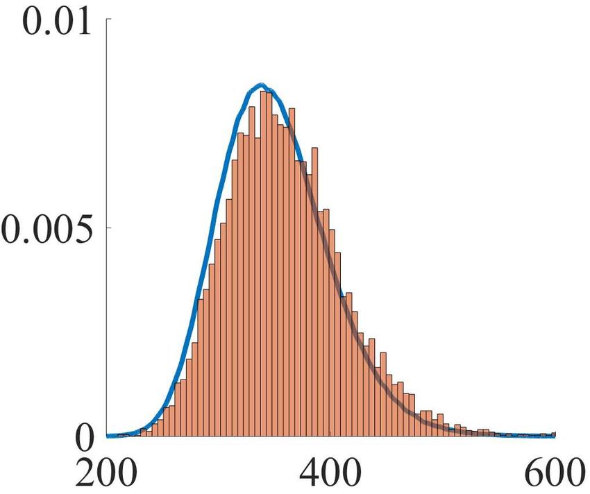
Robust Bayesian Classification Using an Optimistic Score Ratio
Moreno-Torres et al., 2012). ambiguity sets B0 and B1 can be written as
We endeavor in this paper to provide the precise mathemati-
∃f0 ∈ Bρ0 (Pb0 ) ∩ P, f1 ∈ Bρ (P
b1 ) ∩ P :
1
cal model for binary classification with uncertain likelihood
fc (x)πc
under the Bayesian decision analysis framework. Consider B = P : P(Y = c|X = x) = X ∀c ,
a binary classification setting where Y ∈ {0, 1} represents
fc0 (x)πc0
c0 ∈{0,1}
the random class label and X ∈ Rd represents the random
features. With a new observation x to be classified, we con- where the constraint in the set B links the class-conditional
sider the problem of finding an optimal action a ∈ {0, 1}, densities fc and the prior distribution of the class propor-
( tions π to the posterior distribution. Facing with the un-
0 if classify x in class 0, certainty in the posterior distributions, it is reasonable to
a= consider now the distributionally robust problem
1 if classify x in class 1,
min sup aP(Y = 0|X = x) + (1 − a)P(Y = 1|X = x),
to minimize the probability of misclassification by solving a∈{0,1} P∈B
the optimization problem (1)
where the action a is chosen so as to minimize the worst-case
min aP(Y = 0|X = x) + (1 − a)P(Y = 1|X = x), mis-classification probability over all posterior distribution
a∈{0,1}
P ∈ B. The next proposition asserts that the optimal action
where P(Y |X = x) denotes the posterior probability. If a? belongs to the class of ratio decision rule.
a class-proportion prior π and the class-conditional (para- Proposition 1.1 (Optimal action). The optimal action that
metric) densities f0 and f1 are known, then this posterior minimizes the worst-case mis-classification probability (1)
probability can be calculated by using the Bayes’ theo- has the form
rem (Schervish, 1995, Theorem 1.31). Unluckily, we rarely
supf1 ∈Bρ (bP1 )∩P f1 (x)
have access to the true conditional densities in real life.
≥ τ (x),
1 if 1
?
a = supf0 ∈Bρ (bP0 )∩P f0 (x)
To tackle this problem in the data-driven setting, for any 0
0 otherwise,
class c ∈ {0, 1}, the decision maker first forms, to the best
of its belief and on the availability of data, a nominal class-
conditional distribution P bc . We assume now that the true for some threshold τ > 0 that is dependent on x.
class-conditional distribution belongs to an ambiguity set Motivated by this insight from the parametric setting, we
Bρc (Pbc ), defined as a ball, prescribed via an appropriate
now promote the following classification decision rule
measure of dissimilarity, of radius ρc ≥ 0 centered at the
(
nominal distribution P bc in the space of class-conditional
1 if R(x) ≥ τ (x),
probability measures. Besides, we allow to constrain the C(x) =
0 otherwise,
class-conditional distributions to lie in a subspace P of
probability measures to facilitate the injection of optional where R(x) is the ratio defined as
parametric information, should the need arise.
sup `(x, Q)
To avoid any unnecessary measure theoretic complications, Q∈Bρ1 (b
P1 )∩P
we position ourselves temporarily in the parametric setting R(x) , ,
bc ) ∩ P para- sup `(x, Q)
and assume that we can generically write Bρc (P
Q∈Bρ0 (b
P0 )∩P
metrically as
and τ (x) > 0 is a positive threshold which is potentially
bc ) ∩ P = {fc ( · |θc ) : θc ∈ Θc }
Bρc (P ∀c ∈ {0, 1}, dependent on the observation x. The score function `(x, Q)
quantifies the plausibility of observing x under the probabil-
where Θc are non-empty (sub)sets on the finite-dimensional ity measure Q, and the value R(x) quantifies how plausible
parameter space Θ, and Θc satisfy the additional regularity an observation x can be generated by any class-conditional
condition that the density evaluated at point x is strictly probability distribution in Bρ1 (P b1 ) ∩ P relatively to any
positive, i.e., fc (x|θc ) > 0 for all θc ∈ Θc . Notice that the distribution in Bρ0 (Pb0 ) ∩ P. Because both the numerator
parametric subspace of probability distributions P is now and the denominator search for the distribution in the respec-
explicitly described through the set of admissible parameters tive ambiguity set that maximizes the score of observing x,
Θ. If we denote the prior proportions by π0 = π(Y = 0) > R(x) is thus termed the ratio of optimistic scores, and the
0 and π1 = π(Y = 1) > 0, then the ambiguity set over classification decision C is hence called the optimistic score
the posterior distributions induced by the class-conditional ratio classifier.
Robust Bayesian Classification Using an Optimistic Score Ratio

The classifying decision C(x) necessitates the solution of         classification task. These include Bayesian inference using
two optimistic score evaluation problems of the form               synthetic likelihood (Wood, 2010; Price et al., 2018), ap-
                                                                   proximate Bayesian computation (Csilléry et al., 2010; Toni
                        sup       `(x, Q),                 (2)     et al., 2009), variational Bayes inference (Blei et al., 2017;
                     Q∈Bρ (b
                           P)∩P
                                                                   Ong et al., 2018), and composite hypothesis testing using
where the dependence of the input parameters on the label          likelihood ratio (Cox, 1961; 2013). These connections will
c ∈ {0, 1} has been omitted to avoid clutter. The perfor-          be explored in future research.
mance of C depends critically on the specific choice of `          All proofs are relegated to the appendix.
and Bρ (P).
          b Typically, ` is subjectively tailored to the choice
of a parametric or a nonparametric view on the conditional         Notations. We let M be the set of probability measures
distribution, as we shall see later on in this paper. The con-     supported on Rd with finite second moment. The set of
struction of Bρ (P)
                  b is principally governed by choice of the       (symmetric) positive definite matrices is denoted by Sd++ .
dissimilarity measure that specifies the ρ-neighborhood of         For any Q ∈ M, µ ∈ Rd and Σ ∈ Sd++ , we use Q ∼ (µ, Σ)
the nominal distribution P.  b Ideally, Bρ (P)
                                             b should allow a      to express that Q has mean vector µ and covariance matrix
coherent transition between the parametric and nonparamet-         Σ. The d-dimensional identity matrix is denoted by Id .
ric setting via its interaction with the set P. Furthermore, it    The space of Gaussian distributions is denoted by N , and
should render problem (2) computationally tractable with           N (µ, Σ) denotes a Gaussian distribution with mean µ and
meaningful optimal value, and at the same time provide the         covariance matrixΣ. The trace and determinant operator
flexibility to balance between exerting statistical guarantees     are denoted by Tr A and det(A), respectively.
and modelling domain adaptation. These stringent criteria
precludes the utilization of popular dissimilarity measures        2. Moment-based Divergence Ambiguity Set
in the emerging literature. Indeed, the likelihood problem
using the f -divergence (Ben-Tal et al., 2013; Namkoong            We specifically study the construction of the ambiguity set
& Duchi, 2016) delivers unreasonable estimate in the non-          using the following divergence on the space of moments.
parametric setting (Nguyen et al., 2019a, Section 2), the          Definition 2.1 (Moment-based divergence). For any vectors
Wasserstein distance (Mohajerin Esfahani & Kuhn, 2018;             µ1 , µ2 ∈ Rd and matrices Σ1 , Σ2 ∈ Sd++ , the divergence
Kuhn et al., 2019; Blanchet et al., 2019; Gao & Kleywegt,          from the tuple (µ1 , Σ1 ) to the tuple (µ2 , Σ2 ) amounts to
2016; Zhao & Guan, 2018) typically renders the Gaussian
                                                                      D (µ1 , Σ1 ) k (µ2 , Σ2 ) , (µ2 − µ1 )> Σ−1

parametric likelihood problem non-convex, and the maxi-                                                            2 (µ2 − µ1 )
mum mean discrepancy (Iyer et al., 2014; Staib & Jegelka,                              −1

                                                                           + Tr Σ1 Σ2 − log det(Σ1 Σ2 ) − d. −1
2019) usually results in an infinite-dimensional optimization
problem which is challenging to solve. This fact prompts us
to explore an alternative construction of Bρ (P) b that meets      To avoid any confusion, it is worthy to note that contrary
the criteria as mentioned above.                                   to the usual utilization of the term ‘divergence’ to specify a
                                                                   dissimilarity measure on the probability space, in this paper,
The contributions of this paper are summarized as follows.         the divergence is defined on the finite-dimensional space of
                                                                   mean vectors and covariance matrices.
• We introduce a novel ambiguity set based on a divergence
defined on the space of mean vector and covariance matrix.         It is straightforward to show that D is a divergence on Rd ×
We show that this divergence manifests numerous favorable          Sd++ by noticing that D is a sum of the log-determinant
properties and evaluating the optimistic score is equivalent       divergence (Chebbi & Moakher, 2012) from Σ1 to Σ2 and
to solving a non-convex optimization problem. We prove             a non-negative Mahalanobis distance between µ1 and µ2
the asymptotic statistical guarantee of the divergence, which      weighed by Σ2 . As a consequence, D is non-negative, and
directs an optimal calibration the size of the ambiguity set.      perishes to 0 if and only if Σ1 = Σ2 and µ1 = µ2 . With
                                                                   this property, D is an attractive candidate for the divergence
• We show that, despite its inherent non-convexity and             on the joint space of mean vector and covariance matrix
hence intractability, the optimistic score evaluation prob-        of d-dimensional random vectors. One can additionally
lem can be efficiently solved in both nonparametric and            verify that D is affine-invariant in the following sense. Let
parametric Gaussian settings. We reveal that the optimistic        ξ be a d-dimensional random vector and ζ be the affine-
score ratio classifier generalizes the Mahalanobis distance        transformation of ξ, that is, ζ = Aξ + b for an invertible
classifier and the linear/quadratic discriminant analysis.         matrix A and a vector b of matching dimensions, then the
                                                                   value of the divergence D is preserved between the space of
Because evaluating the plausibility of an observation x is         moments of ξ and ζ. In fact, if ξ is a random vector with
a fundamental problem in statistics, the results of this pa-       mean vector µj ∈ Rd and covariance matrix Σj ∈ Sd++ ,
per have far-reaching implications beyond the scope of the         then ζ has mean Aµj + b and covariance matrix AΣj A>
Robust Bayesian Classification Using an Optimistic Score Ratio

for j ∈ {1, 2}, and we have                                                          b then any distribution Q0 with the same
                                                                  Q belongs to Bρ (P),
                                                                 mean vector and covariance matrix with Q also belongs to
    D (µ1 , Σ1 ) k (µ2 , Σ2 )                             (3)     Bρ (P).
                                                                      b Further, Bρ (P)  b embraces all types of probability
                             >                       >            distributions, including discrete, continuous and even mixed

    = D (Aµ1 + b, AΣ1 A ) k (Aµ2 + b, AΣ2 A ) .
                                                                  continuous/discrete distributions.
A direct consequence is that D is also scale-invariant. Fur-
thermore, the divergence D is closely related to the KL diver-    We now delineate a principled approach to solve the op-
gence1 , or the relative entropy, between two non-degenerate      timistic score evaluation problem (2) for a generic score
Gaussian distributions as                                         function ` : Rd × M → R. We denote by M(µ, Σ) the
                                                                  Chebyshev ambiguity set that contains all probability mea-
                                                                  sures with fixed mean vector µ ∈ Rd and fixed covariance

D (µ1 , Σ1 ) k (µ2 , Σ2 ) = 2 KL N (µ1 , Σ1 ) k N (µ2 , Σ2 ) .
                                                                  matrix Σ ∈ Sd++ , that is,
However, we emphasize that D   is not symmetric, and in gen-

eral D (µ1 , Σ1 ) k (µ2 , Σ2 ) 6= D (µ2 , Σ2 ) k (µ1 , Σ1 ) .                 M(µ, Σ) , {Q ∈ M : Q ∼ (µ, Σ)} .
Hence, D is not a distance on Rd × Sd++ .
                                                                  The moment-based divergence ambiguity set Bρ (P)
                                                                                                                b then
For any vector µb ∈ Rd , invertible matrix Σ b ∈ Sd++ and
                                                                  admits an equivalent representation
radius ρ ∈ R+ , we define the uncertainty set Uρ (b
                                                  µ, Σ)
                                                     b over
the mean vector and covariance matrix space as
                                                                                                [
                                                                                Bρ (P)
                                                                                    b =                     M(µ, Σ),
                                                                                           (µ,Σ)∈Uρ (b
                                                                                                     µ,Σ)
  Uρ (b
      µ, Σ)
         b ,                                                                                           b
                                                 (4)
    {(µ, Σ) ∈ Rd × Sd++ : D (b

                                b k (µ, Σ) ≤ ρ}.
                             µ, Σ)                                which is an infinite union of Chebyshev ambiguity sets,
                                                                  where the union operator is taken over all tuples of mean
By definition, Uρ (b
                   µ, Σ)
                      b includes all tuples (µ, Σ) which          vector-covariance matrix belonging to Uρ (bµ, Σ).
                                                                                                                b Leverag-
is of a divergence not bigger than ρ from the tuple (b
                                                     µ, Σ).
                                                        b         ing on this representation, problem (2) can now be decom-
Because D is not symmetric, it is important to note that          posed as a two-layer optimization problem
Uρ (b
    µ, Σ)
       b is defined with the tuple (b µ, Σ)
                                         b being the first
argument of the divergence D, and this uncertainty set can           sup      `(x, Q) =       sup              sup     `(x, Q).
                                                                   Q∈Bρ (b                (µ,Σ)∈Uρ (b b Q∈M(µ,Σ)∩P
                                                                                                    µ,Σ)
be written in a more expressive form as                                  P)
                                                                                                                              (6)
Uρ (b
    µ, Σ)
       b =                                                        The inner subproblem of (6) is a distributionally robust
                                                                  optimization problem with a Chebyshev second moment
   (µ, Σ) ∈ Rd × Sd++ :

                                                                  ambiguity set, hence there is a strong potential to exploit ex-
        b)> Σ−1 (µ − µ        b −1 + log det Σ ≤ ρ

   (µ − µ            b) + Tr ΣΣ
                                                                  istent results from the literature, see Delage & Ye (2010) and
                                                                  Wiesemann et al. (2014), to reformulate this inner problem
for a scalar ρ , ρ + d + log det Σ.b Moreover, one can as-
                                                                  into a finite dimensional convex optimization problem. Un-
sert that Uρ (b
              µ, Σ) is non-convex due to the log-determinant
                 b
                                                                  fortunately, the outer subproblem of (6) is a robust optimiza-
term, and this non-convexity cannot be eliminated using
                                                                  tion problem over a non-convex uncertainty set Uρ (b    µ, Σ),
                                                                                                                              b
the reparametrization to the space of inverse covariance
                                                                  thus the two-layer decomposition problem (6) remains com-
matrices (or equivalently called the precision matrices).
                                                                  putationally intractable in general. As a direct consequence,
Equipped with Uρ (b µ, Σ),
                       b the ambiguity set Bρ (P) b is system-    solving the optimistic score evaluation problem requires an
atically constructed as follows. If the nominal distribution P
                                                             b    intricate adaptation of non-convex optimization techniques
admits a nominal mean vector µ  b and a nominal nondegener-       applied on a case-by-case basis. Two exemplary settings in
ate covariance matrix Σ,b then Bρ (P)b is a ball that contains    which problem (6) can be efficiently solved will be depicted
all probability measures whose mean vector and covariance         subsequently in Sections 3 and 4.
matrix are contained in Uρ (bµ, Σ),
                                b that is,
                                                                  We complete this section by providing the asymptotic sta-
     b , {Q ∈ M : Q ∼ (µ, Σ), (µ, Σ) ∈ Uρ (b                      tistical guarantees of the divergence D, which serves as a
 Bρ (P)                                    µ, Σ)}.
                                              b    (5)
                                                                  potential guideline for the construction of the ambiguity set
                                                                  Bρ (P)
                                                                       b and the tuning of the radius parameter ρ.
The set Bρ (P),
            b by construction, differentiates only through
the information about the first two moments: if a distribution    Theorem 2.2 (Asymptotic guarantee of D). Suppose that
   1
                                                                  a d-dimensional random vector ξ has mean vector m ∈
     If Q1 is absolutely continuous with respect to Q2 , then
the Kullback-Leibler divergence from Q1 to Q2 amounts to
                                                                  Rd , covariance matrix S ∈ Sd++ and admits finite fourth
KL(Q1 k Q2 ) , EQ1 [log dQ1 /dQ2 ], where dQ1 /dQ2 is the         moment under a probability measure P. Let ξbt ∈ Rd , t =
Radon-Nikodym derivative of Q1 with respect to Q2 .               1, . . . , n be independent and identically distributed samples
Robust Bayesian Classification Using an Optimistic Score Ratio
bn ∈ Rd and Σ
of ξ from P. Denote by µ b n ∈ Sd+ the sample probability. While the limiting distribution under the Gaus-
mean vector and sample covariance matrix defined as sian setting is a typical chi-squaredistribution, the general
limiting distribution H > H + Tr Z 2 /2 in Theorem 2.2
n n
1 Xb bn = 1
X does not have any analytical form. This limiting distribution
µ
bn = ξt , Σ (ξbt − µ bn )> . (7)
bn )(ξbt − µ
n t=1 n t=1 can be numerically approximated, for example, via Monte
Carlo simulations. If the i.i.d. assumption of the training
1
Let η = S − 2 (ξ − m) be the isotropic transformation of samples is violated or if we expect a covariate shift at test
the random vector ξ, let H be a d-dimensional Gaussian time, then the radius ρ reflects the modeler’s belief regard-
random vector with mean vector 0 and covariance matrix ing the moment mismatch measured using the divergence
Id , and let Z be a d-by-d random symmetric matrix with the D and in this case, the radius ρ should be considered as an
upper triangle component Zjk (j ≤ k) following a Gaussian exogenous input to the problem.
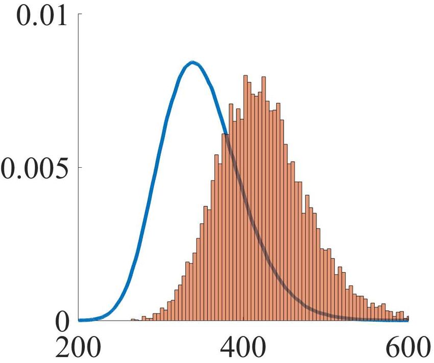
distribution with mean 0 and the covariance coefficient For illustrative purpose, we fix dimension d = 20 and con-
between Zjk and Zj 0 k0 is sider the random vector ξ = Cζ + m, where entries of ζ
are mutually independent and the i-th entry follows a nor- √
cov(Zjk , Zj 0 k0 ) = EP [ηj ηk ηj 0 ηk0 ] − EP [ηj ηk ] EP [ηj 0 ηk0 ]. malized chi-square distribution, i.e., ζi ∼ (χ2 (1) − 1)/ 2.
>
Then the covariance matrix of ξ is S = CC . Notice that
Furthermore, H and Z are jointly Gaussian distributed with by the identity (3), D (bµn , Σn ) k (m, S) is invariant of
b
the covariance between Hi and Zjk as the choice of C and m. We generate 10,000 datasets, each
contains n i.i.d. samples of ξ and calculate for each
dataset
cov(Hi , Zjk ) = EP [ηi ηj ηk ].
the empirical values of n × D (b b n ) k (m, S) . We plot
µn , Σ
1 the empirical distribution of n × D (b
As n ↑ ∞, we have in Figure b n) k
µn , Σ
(m, S) using 10,000 datasets versus the limiting distribu-
n × D (b b n ) k (m, S) tion of H > H + Tr Z 2 /2 for different values of n. One
µn , Σ
1 can observe that for a small sample size (n < 100), there is
−→ H > H + Tr Z 2 in distribution. a perceivable difference between the finite sample distribu-
2
tion and the limiting distribution, but as n becomes larger
We were not able to locate Theorem 2.2 in the existing liter- (n > 100), this mismatch is significantly reduced.
ature. Interestingly, Theorem 2.2 also sheds light upon the
asymptotic behavior of the KL divergence from an empiri-
cal Gaussian distribution N (b
µn , Σ
b n ) to the data-generating
Gaussian distribution N (m, S).
Corollary 2.3 (Asymptotic guarantee of D – Gaussian dis-
tributions). Suppose that ξbt ∈ Rd , t = 1, . . . , n are in-
dependent and identically distributed samples of ξ from
P = N (m, S) for some m ∈ Rd and S ∈ Sd++ . Let
bn ∈ Rd and Σ
µ b n ∈ Sd+ be the sample mean vector and
covariance matrix defined as in (7). As n ↑ ∞, we have (a) n = 30 (b) n = 100
n × KL N (b b n ) k N (m, S)
µn , Σ
1
−→ χ2 (d(d + 3)/2) in distribution,
2
where χ2 (d(d + 3)/2) is a chi-square distribution with
d(d + 3)/2 degrees of freedom.
If we use independent and identically distributed (i.i.d.)
samples to estimate the nominal mean vector and covari- (c) n = 300 (d) n = 1000
b then the radius ρ should be asymptotically
ance matrix of P,
scaled at the rate n−1 as the sample size n increases. In- Figure 1. Empirical distribution of n × D (b b n ) k (m, S)
µn , Σ
deed, Theorem 2.2 and Corollary 2.3 suggest that n−1 is collected from 10,000 datasets (orange
histogram) versus the lim-
the optimal asymptotic rate which ensures that the true but iting distribution H > H + 12 Tr Z 2 obtained by Monte Carlo
simulations (blue curve) for different sample sizes n.
unknown mean vector and covariance matrix of the data-
generating distribution fall into the set Uρ (b
µ, Σ)
b with highRobust Bayesian Classification Using an Optimistic Score Ratio
3. Optimistic Nonparametric Score Because the feasible set Bρ (P)b is not weakly compact, the
existence of an optimal measure that solves the optimistic
We consider in this section the nonparametric setting in likelihood problem on the left-hand side of (8a) is not trivial.
which no prior assumption on the class-conditional distri- However, equation (8a) asserts that this optimal measure
bution is imposed. A major difficulty in this nonparametric exists, and it can be constructed by solving a non-convex op-
setting is the elicitation of a reasonable score function ` that timization problem over the mean vector-covariance matrix
can coherently encapsulate the plausibility of observing x tuple (µ, Σ). Notice that (8a) is a non-convex optimization
over the whole spectrum of admissible Q, including contin-
problem because Uρ (b µ, Σ)
b is a non-convex set. Surpris-
uous, discrete and mixed continuous/discrete distributions,
ingly, one can show that the optimizer of (8a) can be found
while at the same time being amenable for optimization
semi-analytically: the maximizer (µ? , Σ? ) depends only on
purposes. Taking this fact into consideration, we thus posit
a single scalar γ ? through (8c), where γ ? solves the uni-
to choose the score function of the form
variate optimization problem (8d). Because problem (8d) is
convex, γ ? can be efficiently found using a bisection algo-
`(x, Q) ≡ Q({x}),
rithm or using a Newton-Raphson method, and we expose
which is the probability value of the singleton, measurable in Appendix E the first- and second-order derivative of the
set {x} under the measure Q. If Q is a continuous distri- objective function of (8d).
bution, then apparently Q({x}) is zero, hence this score A nonparametric classifier Cnonparam can be formed by utiliz-
function is admittedly not perfect. Nevertheless, it serves as ing the optimistic nonparametric score ratio
a sensible proxy in the nonparametric setting and delivers
competitive performance in machine learning tasks (Nguyen sup Q({x})
Q∈Bρ1 (b
P1 )
et al., 2019b). It is reasonable to set P ≡ M in the non- Rnonparam (x) , , (9)
parametric setting, and with this choice of `, the optimistic sup Q({x})
nonparametric score evaluation problem becomes Q∈Bρ0 (b
P0 )
sup Q({x}), where each nominal class-conditional distribution P bc has
Q∈Bρ (b
P) mean vector µ bc ∈ R and covariance matrix Σc ∈ Sd++ ,
d b
and each ambiguity set Bρc (P bc ) is defined as in (5). The
which is inherently challenging because it is an infinite- results of Theorem 3.1 can be used to compute the numer-
dimensional optimization problem. The next theorem as- ator and denominator of (9), thus the classification deci-
serts that solving the nonparametric optimistic likelihood sion Cnonparam (x) can be efficiently evaluated. In particular,
optimization problem is equivalent to solving a univariate by substituting the expression (8a) into (9), we also find
convex optimization problem.
Theorem 3.1 (Optimistic nonparametric probability). Sup- Rnonparam (x)
b ∼ (b
pose that P µ, Σ) b ∈ Rd and Σ
b for some µ b ∈ Sd++ . For max [1 + (µ − x)> Σ−1 (µ − x)]−1
any ρ ∈ R+ , we have (µ,Σ)∈Uρ1 (b
µ1 ,Σ
b1)
=
max [1 + (µ − x)> Σ−1 (µ − x)]−1
(µ,Σ)∈Uρ0 (b
µ0 ,Σ
b0)
sup Q({x})
Q∈Bρ (b
P) 1+ min (µ − x)> Σ−1 (µ − x)
(µ,Σ)∈Uρ0 (b
µ0 ,Σ
b0)
= max [1 + (µ − x)> Σ−1 (µ − x)]−1 (8a) = .
(µ,Σ)∈Uρ (b
µ,Σ)
b 1+ min (µ − x)> Σ−1 (µ − x)
(µ,Σ)∈Uρ1 (b
µ1 ,Σ
b1)
=[1 + (µ? − x)> (Σ? )−1 (µ? − x)]−1 , (8b)
Suppose that ρ0 = ρ1 = 0 and τ (x) = 1, then the nonpara-
where (µ? , Σ? ) ∈ Rd × Sd++ satisfies metric classifier assigns Cnonparam (x) = 1 whenever
x + γ?µ (b b −1 (b
µ1 − x)> Σ b −1 (b
µ0 − x)> Σ
µ1 − x) ≤ (b µ0 − x),
µ? =
b
, 1 0
1 + γ?
(8c) and Cnonparam (x) = 0 otherwise. In this case, the classi-
1
Σ? = Σ
b+ (x − µ b)> ,
b)(x − µ fier coincides with the class-specific Mahalanobis distance
(1 + γ ? )
classifier (MDC) where Σ b 0 and Σb 1 denote the intra-class
and γ ? ∈ R+ solves the univariate convex optimization nominal covariance matrices. If in addition the nominal co-
problem variance matrices are homogeneous, that is, Σ b0 = Σb 1 , then
this classifier coincides with the Linear Discriminant Anal-
b)> Σ
(x − µ b −1 (x − µ
b) ysis (LDA) (Murphy, 2012, Section 4.2.2). The Bayesian
min γρ − γ log 1 + . (8d) version of LDA can be equivalently obtained from Cnonparam
γ≥0 1+γRobust Bayesian Classification Using an Optimistic Score Ratio
by setting a proper value of τ (x). This important observa- For any ρ ∈ R+ , we have
tion reveals an intimate link between our proposed classifier
Cnonparam using the optimistic nonparametric score ratio and sup L(x, Q)
Q∈Bρ (b
P)∩N
the popular classifiers MDC and LDA. On the one hand,
Cnonparam can now be regarded as a generalization of MDC = max − (µ − x)> Σ−1 (µ − x) − log det Σ
and LDA, which takes into account the statistical impre- (µ,Σ)∈Uρ (b
µ,Σ)
b
cision of the estimated moments and/or the potential shift (11a)
in the moment statistics in test data versus training data ? > ? −1 ? ?
= − (µ − x) (Σ ) (µ − x) − log det Σ , (11b)
distributions. On the other hand, both MDC and LDA now
admit a nonparametric, generative interpretation in which where (µ? , Σ? ) ∈ Rd × Sd++ satisfies
the class-conditional distribution is chosen in the set of all
distributions with the same first- and second-moments as x + γ?µ
µ? =
b
,
the nominal class-conditional measure P bc . This novel in- 1 + γ?
(11c)
terpretation goes beyond the classical Gaussian model, and γ? b γ?
Σ? = Σ+ (x − µ b)> ,
b)(x − µ
it potentially explains the versatile performance of MDC 1+γ ? (1 + γ ? )2
and LDA when the conditional distribution are not normally
distributed as empirically observed in (Lee et al., 2018). and γ ? ∈ R+ solves the univariate convex optimization
problem
4. Optimistic Gaussian Score n 1
min γρ + d(γ + 1) log 1 +
γ≥0 γ
We now consider the optimistic score evaluation problem (11d)
under a parametric setting. For simplicity, we assume that
b)> Σ
(x − µ b −1 (x − µ
b) o
− (1 + γ) log 1 + .
the true class-conditional distributions of the feature belong (1 + γ)
to the family of Gaussian distributions. Thus, a natural
choice of the score value `(x, Q) in this case is the Gaus- Notice that we impose the condition P b ∼ N (b µ, Σ)
b in The-
sian likelihood of an observation x when Q is a Gaussian orem 4.1 to conform with the belief that the true data gen-
distribution with mean µ and covariance matrix Σ, that is, erating distribution is Gaussian. This condition, in fact,
(x − µ)> Σ−1 (x − µ) can be removed without affecting the result presented in
1
`(x, Q) = p exp − . Theorem 4.1. Indeed, for any radius ρ ≥ 0, the ambigu-
(2π)d det Σ 2 ity set Bρ (P)
b by definition contains a Gaussian distribution
with the same mean vector and covariance matrix with the
It is also suitable to set P in problem (2) to the (sub)space nominal distribution P,b and thus the feasible set of (10) is
of Gaussian distributions N and consider the following always non-empty and the value of the optimistic Gaussian
optimistic Gaussian score evaluation problem log-likelihood is always finite. In Appendix E, we provide
the first- and second-order derivatives of the objective func-
sup `(x, Q). (10) tion of (11d), which can be exploited to derive efficient
Q∈Bρ (b
P)∩N
algorithm to solve the convex program (11d).
One can verify that the maximizer of problem (10) coincides Returning to the construction of the classifier, one can now
with the maximizer of construct the classifier CN (x) using the optimistic Gaussian
score ratio RN (x) expressed by
sup L(x, Q),
Q∈Bρ (b
P)∩N sup `(x, Q)
Q∈Bρ1 (b
P1 )∩N
RN (x) ,
where L is the translated Gaussian log-likelihood defined as sup `(x, Q)
Q∈Bρ0 (b
P0 )∩N
d
1
L(x, Q) = 2 log `(x, Q) + log(2π) exp 2 sup L(x, Q)
2 Q∈Bρ1 (b
P1 )∩N
= −(µ − x)> Σ−1 (µ − x) − log det Σ. = , (12)
1
exp 2 sup L(x, Q)
Q∈Bρ0 (b
P0 )∩N
Theorem 4.1 is a counterpart to the optimistic nonparametric
likelihood presented in Theorem 3.1. where each nominal distribution P
bc is a Gaussian distri-
Theorem 4.1 (Optimistic Gaussian log-likelihood). Sup- bc ∈ Rd and covariance matrix
bution with mean vector µ
b ∼ N (b
pose that P µ, Σ) b ∈ Rd and Σ
b for some µ b ∈ Sd .
++
b c ∈ Sd , and each ambiguity set Bρ (P
Σ ++ c
bc ) is defined asRobust Bayesian Classification Using an Optimistic Score Ratio
in (5). Theorem 4.1 can be readily applied to evaluate the for optimistic Gaussian decision rule, the decision bound-
value RN (x), and classify x using CN (x). Furthermore, aries look similar across different radii; while in nonpara-
suppose that ρ0 = ρ1 = 0 and τ (x) = 1, then the result- metric case, the decision boundaries exhibit different shapes.
ing classifier recovers the Quadratic Discriminant Analy- We then consider the case with distinct radii by setting
sis (Murphy, 2012, Section 4.2.1). The Bayesian version of ρ
~ = (ρ0 , ρ1 ) = (0.1, 1.0) and ρ~ = (ρ0 , ρ1 ) = (1.0, 0.1).
the QDA can be equivalently obtained from CN by setting a Further, we fix the threshold to a constant τ (x) = τ ? for a
proper value for τ (x). scalar τ ? ∈ R+ that solves
It is imperative to elaborate on the improvement of Theo- n0
X n1
X
rem 4.1 compared to the result reported in Nguyen et al. max x0,i ) < τ }+
1{R(b x1,i ) ≥ τ },
1{R(b (13)
τ ≥0
(2019a, Section 3). While both results are related to the eval- i=1 i=1
uation of the optimistic Gaussian log-likelihood, Nguyen
et al. (2019a, Theorem 3.2) restricts the mean vector to its where 1{ · } is the indicator function. The decision bound-
nominal value and optimizes only over the covariance ma- aries are plotted in Figure 3. We find the decision boundaries
trix. On the other hand, Theorem 4.1 of this paper optimizes have different shapes for different decision rules and for dif-
over both the mean vector and the covariance matrix, thus ferent choices of radii.
provides full flexibility to choose the optimal values of all
sufficient statistics of the family of Gaussian distributions.
From a technical standpoint, the non-convexity is overcome
in Nguyen et al. (2019a, Theorem 3.2) through a simple
change of variables; nonetheless, the proof of Theorem 4.1
demands an additional layer of duality arguments to disen-
tangle the multiplicative terms between µ and Σ in both the
objective function L and the divergence D. By inspecting
the expressions in (11c), one can further notice that in gen-
eral the optimal solution µ? is distinct from the nominal
mean µ b, this observation suggests that optimizing jointly (a) Gaussian, ρb = 0.5 (b) Nonparametric, ρb = 0.5
over (µ, Σ) is indeed more powerful than optimizing simply
over Σ from a theoretical perspective.
5. Numerical Results
All experiments are run on a standard laptop with 1.4 GHz
Intel Core i5 and 8GB of memory, the codes and datasets are
available at https://github.com/nian-si/bsc.
5.1. Decision Boundaries
In this section, we visualize the classification decision (c) Gaussian, ρb = 0.7 (d) Nonparametric, ρb = 0.7
boundaries generated by the classifiers Cnonparam proposed
in Section 3 and CN proposed in Section 4 using synthetic Figure 2. Decision boundaries for different ρb. Red/blue regions
data. To ease the exposition, we consider a two dimensional indicate the class partitions, black dots locate the mean, and white
feature space d = 2 and the class-conditional distributions dashed ellipsoids draw the class-conditional density contours.
are Gaussian of the form
5.2. Real Data Experiments
0 1 1 0.5
X|Y = 0 ∼ N ,Id , X|Y = 1 ∼ N , .
1 0 0.5 1 In our experiments, we first compute the nominal mean
We sample i.i.d. data points {b nc
xc,i }i=1 in each c ∈ {0, 1} by empirical average and we use the Ledoit-Wolf covari-
with n0 = n1 = 1000 as the training set, then estimate the ance estimator (Ledoit & Wolf, 2004) to compute a well-
nominal mean µ bc and the nominal covariance matrix Σc for
b conditioned nominal covariance matrix. We experiment two
each class c ∈ {0, 1} using the sample average formula (7). methods of tuning the radii ρ of the ambiguity sets: using
cross-validation on training data, or using the quantile of
We first consider when the ambiguity sets have the same ra- the limiting distribution in Corollary 2.3. Specifically, for
dius, i.e., ρ0 = ρ1 = ρb and fix the threshold τ (x) = 1 for ev- the second criteria, we choose
ery x. Figure 2 shows the optimistic Gaussian and nonpara-
metric decision boundaries for ρb ∈ {0.5, 0.7}. We find that ρc = n−1 2
c χα (d(d + 3)/2) ∀c ∈ {0, 1},Robust Bayesian Classification Using an Optimistic Score Ratio
Table 1. Correct classification rate on the benchmark date sets. Bold number corresponds to the best performance in each dataset.
DATASET GQDA, CV GQDA, CLT NPQDA, CV NPQDA, CLT KQDA RQDA SQDA
AUSTRALIAN 85.38 84.91 85.84 85.03 85.38 85.61 85.37
BANKNOTE 99.83 99.33 99.3 99.83 99.8 99.77 99.83
CLIMATE MODEL 94.81 89.33 93.92 90.37 92.59 94.07 93.92
CYLINDER 71.04 70.81 71.11 70.89 71.11 71.11 70.67
DIABETIC 75.52 73.49 76.09 76.30 75.47 75.00 74.32
FOURCLASS 77.82 79.26 80.28 78.98 78.38 79.07 78.84
HABERMAN 74.93 75.33 75.45 75.45 74.94 74.80 74.16
HEART 81.76 83.09 83.09 81.91 81.76 81.91 83.68
HOUSING 91.66 90.55 91.81 91.50 91.66 91.66 91.97
ILPD 68.84 69.52 69.25 68.15 69.18 67.94 69.52
MAMMOGRAPHIC MASS 80.39 80.00 79.90 79.61 79.95 80.05 80.24
Algorithm 1 Optimistic score ratio classification
xc,i }ni=1
1: Input: datasets {b c
for c ∈ {0, 1}. A test data x.
2: Compute the nominal mean and the nominal covariance
matrix
3: Compute the radii ρc ← n−1 2
c χ0.5 (d(d + 3)/2).
4: Compute the optimistic ratio R(b xc,i ) for every x
bc,i
5: Compute the threshold τ ? that solves (13).
6: Output: classification label 1{R(x) ≥ τ }.
(a) Gaussian, ρ
~ = (0.1, 1.0) (b) Nonparametric, ρ
~ = (0.1, 1.0)
using Algorithm 1 is comparable in terms of test accuracy to
classifying with cross-validating on the tuning parameters.
We test the performance of our classification rules on vari-
ous datasets from the UCI repository (Dua & Graff, 2017).
Specifically, we compare the following methods:
• Gaussian QDA (GQDA) and Nonparametric QDA
(NPQDA): Our classifiers CN and Cnonparam ;
• Kullback-Leibler QDA (KQDA): The classifier based on
(c) Gaussian, ρ
~ = (1.0, 0.1) (d) Nonparametric, ρ
~ = (1.0, 0.1)
KL ambiguity sets with fixed mean (Nguyen et al., 2019a);
Figure 3. Decision boundaries with distinct radii. Indications are • Regularized QDA (RQDA): The regularized QDA based
verbatim from Figure 2. on the linear shrinkage covariance estimator Σ
b c + ρc I d ;
where nc is the number of training samples in class c and • Sparse QDA (SQDA): The sparse QDA based on the
χ2α (d(d + 3)/2) is the α-quantile of the chi-square distri- graphical lasso covariance estimator (Friedman et al., 2008)
bution with d(d + 3)/2 degrees of freedom. Notice that with parameter ρc .
for large degrees of freedom, the chi-square distribution
concentrates around the mean, because a chi-square ran- For GQDA and NPQDA, we also compare the performance
dom variable with k degrees of freedom is the sum of k of different strategies to choose the radii ρ using cross-
i.i.d. χ2 (1). The optimal asymptotic value of the radius validation (CV) and selection based on Theorem 2.2 (CLT).
ρc is therefore insensitive to the choice of α, so we select For all methods that need cross-validation, we randomly
numerically α = 0.5 in our experiments. We tune the thresh- select 75% of the data for training and the remaining 25%
old to maximize the training accuracy following (13) after for testing. The size of the ambiguity sets and the reg-
computing the ratio value for each training sample. The ularization parameter are selected using stratified 5-fold
whole procedure is summarized in Algorithm 1. In partic- cross-validation. Furthermore, to promote a fair compari-
ular, this algorithm trains the parameters using only one son, we tune the threshold for every method using (13). The
pass over the training samples, which makes it significantly performance of the classifiers is measured by the average
faster than the cross-validation approach. We observe em- correct classification rate (CCR) on the validation set. The
pirically in most cases that the performance of classifying average CCR score over 10 trials are reported in Table 1.Robust Bayesian Classification Using an Optimistic Score Ratio
Acknowledgements Csilléry, K., Blum, M. G., Gaggiotti, O. E., and François, O.
Approximate Bayesian Computation (ABC) in practice.
We gratefully acknowledge support from the following NSF Trends in Ecology & Evolution, 25(7):410 – 418, 2010.
grants 1915967, 1820942, 1838676 as well as the China
Merchants Bank. Delage, E. and Ye, Y. Distributionally robust optimization
under moment uncertainty with application to data-driven
References problems. Operations Research, 58(3):595–612, 2010.
Ben-Tal, A., den Hertog, D., De Waegenaere, A., Melenberg, Dua, D. and Graff, C. UCI machine learning repository,
B., and Rennen, G. Robust solutions of optimization prob- 2017. URL http://archive.ics.uci.edu/ml.
lems affected by uncertain probabilities. Management
Science, 59(2):341–357, 2013. Friedman, J., Hastie, T., and Tibshirani, R. Sparse inverse
covariance estimation with the graphical lasso. Biostatis-
Bhagat, S., Cormode, G., and Muthukrishnan, S. Node tics, 9(3):432–441, 2008.
classification in social networks. In Social Network Data
Gao, R. and Kleywegt, A. J. Distributionally robust stochas-
Analytics, pp. 115–148. Springer, 2011.
tic optimization with Wasserstein distance. arXiv preprint
Bickel, S., Brückner, M., and Scheffer, T. Discriminative arXiv:1604.02199, 2016.
learning under covariate shift. Journal of Machine Learn- Ghosh, A. and Basu, A. Robust Bayes estimation using
ing Research, 10(Sep):2137–2155, 2009. the density power divergence. Annals of the Institute of
Statistical Mathematics, 68(2):413–437, 2016.
Bissiri, P. G., Holmes, C. C., and Walker, S. G. A general
framework for updating belief distributions. Journal of Gretton, A., Smola, A., Huang, J., Schmittfull, M., Borg-
the Royal Statistical Society: Series B (Statistical Method- wardt, K., and Schölkopf, B. Covariate shift and local
ology), 78(5):1103–1130, 2016. learning by distribution matching, pp. 131–160. MIT
Press, 2009.
Blanchet, J., Kang, Y., and Murthy, K. Robust wasserstein
profile inference and applications to machine learning. Grünwald, P. The safe Bayesian. In International Con-
Journal of Applied Probability, 56(3):830–857, 2019. ference on Algorithmic Learning Theory, pp. 169–183.
Springer, 2012.
Blei, D. M., Kucukelbir, A., and McAuliffe, J. D. Varia-
tional inference: A review for statisticians. Journal of Holmes, C. and Walker, S. Assigning a value to a power
the American Statistical Association, 112(518):859–877, likelihood in a general Bayesian model. Biometrika, 104
2017. (2):497–503, 2017.
Bodendorf, F. and Kaiser, C. Detecting opinion leaders and Iyer, A., Nath, S., and Sarawagi, S. Maximum mean dis-
trends in online social networks. In Proceedings of the crepancy for class ratio estimation: Convergence bounds
2nd ACM Workshop on Social Web Search and Mining, and kernel selection. In Proceedings of the 31st Interna-
pp. 65–68, 2009. tional Conference on Machine Learning, volume 32, pp.
530–538, 2014.
Chebbi, Z. and Moakher, M. Means of Hermitian
Jewson, J., Smith, J. Q., and Holmes, C. Principles of
positive-definite matrices based on the log-determinant α-
Bayesian inference using general divergence criteria. En-
divergence function. Linear Algebra and its Applications,
tropy, 20(6):442, 2018.
436(7):1872 – 1889, 2012.
Knoblauch, J. Robust deep Gaussian processes. arXiv
Chérief-Abdellatif, B.-E. and Alquier, P. MMD-Bayes: Ro- preprint arXiv:1904.02303, 2019.
bust Bayesian estimation via maximum mean discrepancy.
arXiv preprint arXiv:1909.13339, 2019. Knoblauch, J., Jewson, J., and Damoulas, T. Generalized
variational inference. arXiv preprint arXiv:1904.02063,
Cox, D. R. Tests of separate families of hypotheses. In 2019.
Proceedings of the Fourth Berkeley Symposium on Math-
ematical Statistics and Probability, pp. 105–123, 1961. Kuhn, D., Esfahani, P. M., Nguyen, V. A., and Shafieezadeh-
Abadeh, S. Wasserstein distributionally robust optimiza-
Cox, D. R. A return to an old paper: ‘tests of separate tion: Theory and applications in machine learning. IN-
families of hypotheses’. Journal of the Royal Statistical FORMS TutORials in Operations Research, pp. 130–166,
Society: Series B, 75(2):207–215, 2013. 2019.Robust Bayesian Classification Using an Optimistic Score Ratio
Ledoit, O. and Wolf, M. A well-conditioned estimator Rippl, T., Munk, A., and Sturm, A. Limit laws of the
for large-dimensional covariance matrices. Journal of empirical Wasserstein distance: Gaussian distributions.
Multivariate Analysis, 88(2):365 – 411, 2004. Journal of Multivariate Analysis, 151:90–109, 2016.
Lee, K., Lee, K., Lee, H., and Shin, J. A simple unified Schervish, M. J. Theory of Statistics. Springer, 1995.
framework for detecting out-of-distribution samples and
Staib, M. and Jegelka, S. Distributionally robust optimiza-
adversarial attacks. In Advances in Neural Information
tion and generalization in kernel methods. In Advances
Processing Systems 31, pp. 7167–7177, 2018.
in Neural Information Processing Systems 32, pp. 9134–
Miller, J. W. and Dunson, D. B. Robust Bayesian infer- 9144, 2019.
ence via coarsening. Journal of the American Statistical Tomar, D. and Agarwal, S. A survey on data mining ap-
Association, 114(527):1113–1125, 2019. proaches for healthcare. International Journal of Bio-
Science and Bio-Technology, 5(5):241–266, 2013.
Mohajerin Esfahani, P. and Kuhn, D. Data-driven distribu-
tionally robust optimization using the Wasserstein met- Toni, T., Welch, D., Strelkowa, N., Ipsen, A., and Stumpf,
ric: Performance guarantees and tractable reformulations. M. P. Approximate Bayesian computation scheme for
Mathematical Programming, 171(1-2):115–166, 2018. parameter inference and model selection in dynamical
systems. Journal of The Royal Society Interface, 6(31):
Moreno-Torres, J., Raeder, T., Alaiz-Rodrı́guez, R., Chawla, 187–202, 2009.
N., and Herrera, F. A unifying view on dataset shift
in classification. Pattern Recognition, 45(1):521 – 530, Walker, S. G. Bayesian inference with misspecified models.
2012. Journal of Statistical Planning and Inference, 143(10):
1621–1633, 2013.
Murphy, K. Machine Learning: A Probabilistic Perspective.
MIT Press, 2012. Wiesemann, W., Kuhn, D., and Sim, M. Distributionally
robust convex optimization. Operations Research, 62(6):
Namkoong, H. and Duchi, J. C. Stochastic gradient 1358–1376, 2014.
methods for distributionally robust optimization with f-
Wood, S. N. Statistical inference for noisy nonlinear eco-
divergences. In Advances in Neural Information Process-
logical dynamic systems. Nature, 466:1102–1104, 2010.
ing Systems 29, pp. 2208–2216, 2016.
Zhao, C. and Guan, Y. Data-driven risk-averse stochastic op-
Naraei, P., Abhari, A., and Sadeghian, A. Application of timization with Wasserstein metric. Operations Research
multilayer perceptron neural networks and support vector Letters, 46(2):262 – 267, 2018.
machines in classification of healthcare data. In 2016 Fu-
ture Technologies Conference, pp. 848–852. IEEE, 2016. Zhu, W., Miao, J., Hu, J., and Qing, L. Vehicle detection
in driving simulation using extreme learning machine.
Nguyen, V. A., Shafieezadeh-Abadeh, S., Yue, M.-C., Kuhn, Neurocomputing, 128:160–165, 2014.
D., and Wiesemann, W. Calculating optimistic likeli-
hoods using (geodesically) convex optimization. In Ad-
vances in Neural Information Processing Systems 32, pp.
13942–13953, 2019a.
Nguyen, V. A., Shafieezadeh-Abadeh, S., Yue, M.-C., Kuhn,
D., and Wiesemann, W. Optimistic distributionally robust
optimization for nonparametric likelihood approximation.
In Advances in Neural Information Processing Systems
32, pp. 15872–15882, 2019b.
Ong, V. M. H., Nott, D. J., Tran, M.-N., Sisson, S. A.,
and Drovandi, C. C. Variational Bayes with synthetic
likelihood. Statistics and Computing, 28(4):971–988,
2018.
Price, L. F., Drovandi, C. C., Lee, A., and Nott, D. J.
Bayesian synthetic likelihood. Journal of Computational
and Graphical Statistics, 27(1):1–11, 2018.You can also read