VARIATIONAL INFERENCE OF DISENTANGLED LATENT CONCEPTS FROM UNLABELED OBSERVATIONS - OpenReview
←
→
Page content transcription
If your browser does not render page correctly, please read the page content below
Published as a conference paper at ICLR 2018

VARIATIONAL I NFERENCE OF D ISENTANGLED L ATENT
C ONCEPTS FROM U NLABELED O BSERVATIONS
 Abhishek Kumar, Prasanna Sattigeri, Avinash Balakrishnan
 IBM Research AI
 Yorktown Heights, NY
 {abhishk,psattig,avinash.bala}@us.ibm.com

                                                     A BSTRACT

             Disentangled representations, where the higher level data generative factors are
             reflected in disjoint latent dimensions, offer several benefits such as ease of deriving
             invariant representations, transferability to other tasks, interpretability, etc. We
             consider the problem of unsupervised learning of disentangled representations from
             large pool of unlabeled observations, and propose a variational inference based
             approach to infer disentangled latent factors. We introduce a regularizer on the
             expectation of the approximate posterior over observed data that encourages the
             disentanglement. We also propose a new disentanglement metric which is better
             aligned with the qualitative disentanglement observed in the decoder’s output. We
             empirically observe significant improvement over existing methods in terms of
             both disentanglement and data likelihood (reconstruction quality).

1       I NTRODUCTION

Feature representations of the observed raw data play a crucial role in the success of machine learning
algorithms. Effective representations should be able to capture the underlying (abstract or high-level)
latent generative factors that are relevant for the end task while ignoring the inconsequential or
nuisance factors. Disentangled feature representations have the property that the generative factors
are revealed in disjoint subsets of the feature dimensions, such that a change in a single generative
factor causes a highly sparse change in the representation. Disentangled representations offer several
advantages – (i) Invariance: it is easier to derive representations that are invariant to nuisance factors
by simply marginalizing over the corresponding dimensions, (ii) Transferability: they are arguably
more suitable for transfer learning as most of the key underlying generative factors appear segregated
along feature dimensions, (iii) Interpretability: a human expert may be able to assign meanings to
the dimensions, (iv) Conditioning and intervention: they allow for interpretable conditioning and/or
intervention over a subset of the latents and observe the effects on other nodes in the graph. Indeed,
the importance of learning disentangled representations has been argued in several recent works
(Bengio et al., 2013; Lake et al., 2016; Ridgeway, 2016).
Recognizing the significance of disentangled representations, several attempts have been made in this
direction in the past (Ridgeway, 2016). Much of the earlier work assumes some sort of supervision in
terms of: (i) partial or full access to the generative factors per instance (Reed et al., 2014; Yang et al.,
2015; Kulkarni et al., 2015; Karaletsos et al., 2015), (ii) knowledge about the nature of generative
factors (e.g, translation, rotation, etc.) (Hinton et al., 2011; Cohen & Welling, 2014), (iii) knowledge
about the changes in the generative factors across observations (e.g., sparse changes in consecutive
frames of a Video) (Goroshin et al., 2015; Whitney et al., 2016; Fraccaro et al., 2017; Denton &
Birodkar, 2017; Hsu et al., 2017), (iv) knowledge of a complementary signal to infer representations
that are conditionally independent of it1 (Cheung et al., 2014; Mathieu et al., 2016; Siddharth et al.,
2017). However, in most real scenarios, we only have access to raw observations without any
supervision about the generative factors. It is a challenging problem and many of the earlier attempts
have not been able to scale well for realistic settings (Schmidhuber, 1992; Desjardins et al., 2012;
Cohen & Welling, 2015) (see also, Higgins et al. (2017)).
    1
        The representation itself can still be entangled in rest of the generative factors.

                                                            1
Published as a conference paper at ICLR 2018
Recently, Chen et al. (2016) proposed an approach to learn a generative model with disentangled
factors based on Generative Adversarial Networks (GAN) (Goodfellow et al., 2014), however
implicit generative models like GANs lack an effective inference mechanism2 , which hinders its
applicability to the problem of learning disentangled representations. More recently, Higgins et al.
(2017) proposed an approach based on Variational AutoEncoder (VAE) Kingma & Welling (2013)
for inferring disentangled factors. The inferred latents using their method (termed as β-VAE ) are
empirically shown to have better disentangling properties, however the method deviates from the
basic principles of variational inference, creating increased tension between observed data likelihood
and disentanglement. This in turn leads to poor quality of generated samples as observed in (Higgins
et al., 2017).
In this work, we propose a principled approach for inference of disentangled latent factors based on
the popular and scalable framework of amortized variational inference (Kingma & Welling, 2013;
Stuhlmüller et al., 2013; Gershman & Goodman, 2014; Rezende et al., 2014) powered by stochastic
optimization (Hoffman et al., 2013; Kingma & Welling, 2013; Rezende et al., 2014). Disentanglement
is encouraged by introducing a regularizer over the induced inferred prior. Unlike β-VAE (Higgins
et al., 2017), our approach does not introduce any extra conflict between disentanglement of the
latents and the observed data likelihood, which is reflected in the overall quality of the generated
samples that matches the VAE and is much better than β-VAE. This does not come at the cost
of higher entanglement and our approach also outperforms β-VAE in disentangling the latents as
measured by various quantitative metrics. We also propose a new disentanglement metric, called
Separated Attribute Predictability or SAP, which is better aligned with the qualitative disentanglement
observed in the decoder’s output compared to the existing metrics.
2 F ORMULATION
We start with a generative model of the observed data that first samples a latent variable z ∼ p(z), and
an observation is generated by sampling from pθ (x|z). The joint density of latents and observations
is denoted as pθ (x, z) = p(z)pθ (x|z). The problem of inference is to compute the posterior of
the latents conditioned on the observations, i.e., pθ (z|x) = R ppθθ(x,z)dz
(x,z)
. We assume that we are
given a finite set of samples (observations) from the true data distribution p(x). In most practical
scenarios involving high dimensional and complex data, this computation is intractable and calls for
approximate inference. Variational inference takes an optimization based approach to this, positing a
family D of approximate densities over the latents and reducing the approximate inference problem
to finding a member density that minimizes the Kullback-Leibler divergence to the true posterior,
i.e., qx∗ = minq∈D KL(q(z)kpθ (z|x)) (Blei et al., 2017). The idea of amortized inference (Kingma
& Welling, 2013; Stuhlmüller et al., 2013; Gershman & Goodman, 2014; Rezende et al., 2014) is
to explicitly share information across inferences made for each observation. One successful way of
achieving this for variational inference is to have a so-called recognition model, parameterized by φ,
that encodes an inverse map from the observations to the approximate posteriors (also referred as
variational autoencoder or VAE) (Kingma & Welling, 2013; Rezende et al., 2014). The recognition
model parameters are learned by optimizing the problem minφ Ex KL(qφ (z|x)kpθ (z|x)), where the
outer expectation is over the true data distribution p(x) which we have samples from. This can be
shown as equivalent to maximizing what is termed as evidence lower bound (ELBO):
arg min Ex KL(qφ (z|x)kpθ (z|x)) = arg max Ex Ez∼qφ (z|x) [log pθ (x|z)] − KL(qφ (z|x)kp(z))
θ,φ θ,φ
(1)
The ELBO (the objective at the right side of Eq. 1) lower bounds the log-likelihood of observed
data, and the gap vanishes at the global optimum. Often, the density forms of p(z) and qφ (z|x) are
chosen such that their KL-divergence can be written analytically in a closed-form expression (e.g.,
p(z) is N (0, I) and qφ (z|x) is N (µφ (x), Σφ (x))) (Kingma & Welling, 2013). In such cases, the
ELBO can be efficiently optimized (to a stationary point) using stochastic first order methods where
both expectations are estimated using mini-batches. Further, in cases when qφ (·) can be written as a
continuous transformation of a fixed base distribution (e.g., the standard normal distribution), a low
2
There have been a few recent attempts in this direction for visual data (Dumoulin et al., 2016; Donahue
et al., 2016; Kumar et al., 2017) but often the reconstructed samples are semantically quite far from the input
samples, sometimes even changing in the object classes.
2Published as a conference paper at ICLR 2018
variance estimate of the gradient over φ can be obtained by coordinate transformation (also referred
as reparametrization) (Fu, 2006; Kingma & Welling, 2013; Rezende et al., 2014).
2.1 G ENERATIVE STORY: DISENTANGLED PRIOR
Most VAE based generative models for real datasets (e.g., text, images, etc.) already work with a
relatively simple and disentangled prior p(z) having no interaction among the latent dimensions (e.g.,
the standard Gaussian N (0, I)) (Bowman et al., 2015; Miao et al., 2016; Hou et al., 2017; Zhao et al.,
2017). The complexity of the observed data is absorbed in the conditional distribution pθ (x|z) which
encodes the interactions among the latents. Hence, as far as the generative modeling is concerned,
disentangled prior sets us in the right direction.
2.2 I NFERRING DISENTANGLED LATENTS
Although the generative model starts with a disentangled prior, our main objective is to infer disentan-
gled latents which are potentially conducive for various goals mentioned in Sec. 1 (e.g., invariance,
transferability, interpretability). To this end, we consider the density over the inferred latents induced
by the approximate posterior inference mechanism,
Z
qφ (z) = qφ (z|x)p(x)dx, (2)
which we will subsequently refer to as the inferred prior or expected variational posterior (p(x) is
the true data distribution that we have only samples from). Q For inferring disentangled factors, this
should be factorizable along the dimensions, i.e., qφ (z) = i qi (zi ), or equivalently qi|j (zi |zj ) =
qi (zi ), ∀ i, j. This can be achieved by minimizing a suitable distance between the inferred prior
Rqφ (z) and the disentangled generative prior p(z). We can also define expected posterior as pθ (z) =
pθ (z|x)p(x)dx. If we take KL-divergence as our choice of distance, by relying on its pairwise
convexity (i.e., KL(λp1 + (1 − λ)p2 kλq1 + (1 − λ)q2 ) ≤ λKL(p1 kq1 ) + (1 − λ)KL(p2 kq2 ))
(Van Erven & Harremos, 2014), we can show that the distance between qφ (z) and pθ (z) is bounded
by the objective of the variational inference:
KL(qφ (z)kpθ (z)) = KL(Ex∼p(x) qφ (z|x)kEx∼p(x) pθ (z|x)) ≤ Ex∼p(x) KL(qφ (z|x)kpθ (z|x)).
(3)
In general, the prior p(z) and expected
R posterior pθ (z) will be different, although they may be close
(they will be same when pθ (x) = pθ (x|z)p(z)dz is equal to p(x)). Hence, variational posterior
inference of latent variables with disentangled prior naturally encourages inferring factors that are
close to being disentangled. We think this is the reason that the original VAE (Eq. (1)) has also
been observed to exhibit some disentangling behavior on simple datasets such as MNIST (Kingma &
Welling, 2013). However, this behavior does not carry over to more complex datasets (Aubry et al.,
2014; Liu et al., 2015; Higgins et al., 2017), unless extra supervision on the generative factors is
provided (Kulkarni et al., 2015; Karaletsos et al., 2015). This can be due to: (i) p(x) and pθ (x) being
far apart which in turn causes p(z) and pθ (z) being far apart, and (ii) the non-convexity of the ELBO
objective which prevents us from achieving the global minimum of Ex KL(qφ (z|x)kpθ (z|x)) (which
is 0 and implies KL(qφ (z)kpθ (z)) = 0). In other words, maximizing the ELBO (Eq. (1)) might also
result in reducing the value of KL(qφ (z)kp(z)), however, due to the aforementioned reasons, the
gap between KL(qφ (z)kp(z)) and Ex KL(qφ (z|x)kpθ (z|x)) could be large at the stationary point
of convergence. Hence, minimizing KL(qφ (z)kp(z)) or any other suitable distance D(qφ (z), p(z))
explicitly will give us better control on the disentanglement. This motivates us to add D(qφ (z)kp(z))
as part of the objective to encourage disentanglement during inference, i.e.,
max Ex Ez∼qφ (z|x) [log pθ (x|z)] − KL(qφ (z|x)kp(z)) − λ D(qφ (z)kp(z)), (4)
θ,φ
where λ controls its contribution to the overall objective. We refer to this as DIP-VAE (for Disentan-
gled Inferred Prior) subsequently.
Optimizing (4) directly is not tractable if D(·, ·) is taken to be the KL-divergence KL(qφ (z)kp(z)),
which does not have a closed-form expression. One possibility is use the variational formulation of
the KL-divergence (Nguyen et al., 2010; Nowozin et al., 2016) that needs only samples from qφ (z)
and p(z) to estimate a lower bound to KL(qφ (z)kp(z)). However, this would involve optimizing for
3Published as a conference paper at ICLR 2018
a third set of parameters ψ for the KL-divergence estimator, and would also change the optimization
to a saddle-point (min-max) problem which has its own optimization challenges (e.g., gradient
vanishing as encountered in training generative adversarial networks with KL or Jensen-Shannon
(JS) divergences (Goodfellow et al., 2014; Arjovsky & Bottou, 2017)). Taking D to be another
suitable distance between qφ (z) and p(z) (e.g., integral probability metrics like Wasserstein distance
(Sriperumbudur et al., 2009)) might alleviate some of these issues (Arjovsky et al., 2017) but will
still involve complicating the optimization to a saddle point problem in three set of parameters3 . It
should also be noted that using these variational forms of the distances will still leave us with an
approximation to the actual distance.
We adopt a simpler yet effective alternative of matching the moments of the two distributions.
Matching the covariance of the two distributions will amount to decorrelating the dimensions of
z ∼ qφ (z) if p(z) is N (0, I). Let us denote Covq(z) [z] := Eq(z) (z − Eq(z) [z])(z − Eq[z] (z))> .
By the law of total covariance, the covariance of z ∼ qφ (z) is given by
Covqφ (z) [z] = Ep(x) Covqφ (z|x) [z] + Covp(x) Eqφ (z|x) [z] , (5)
where Eqφ (z|x) [z] and Covqφ (z|x) [z] are random variables that are functions of the random variable
x (z is marginalized over). Most existing work on the VAE models uses qφ (z|x) having the form
N (µφ (x), Σφ (x)), where µφ (x) and Σφ (x) are the outputs of a deep neural net parameterized by
φ. In this case Eq. (5) reduces to Covqφ (z) [z] = Ep(x) [Σφ (x)] + Covp(x) [µφ (x)], which we want
to be close to the Identity matrix. For simplicity, we choose entry-wise squared `2 -norm as the
measure of proximity. Further, Σφ (x) is commonly taken to be a diagonal matrix which means that
cross-correlations (off-diagonals) between the latents are due to only Covp(x) [µφ (x)]. This suggests
two possible options for the disentangling regularizer: (i) regularizing only Covp(x) [µφ (x)] which
we refer as DIP-VAE-I, (ii) regularizing Covqφ (z) [z] which we refer as DIP-VAE-II. Penalizing just
the off-diagonals in both cases will lead to lowering the diagonal entries of Covp(x) [µφ (x)] as the
ij’th off-diagonal is really a derived attribute obtained by multiplying the square-roots of i’th and
j’th diagonals (for each example x ∼ p(x), followed by averaging over all examples). This can be
compensated in DIP-VAE-I by a regularizer on the diagonal entries of Covp(x) [µφ (x)] which pulls
these towards 1. We opt for two separate hyperparameters controlling the relative importance of the
loss on the diagonal and off-diagonal entries as follows:
X 2 X 2
max ELBO(θ, φ) − λod Covp(x) [µφ (x)] ij − λd Covp(x) [µφ (x)] ii − 1 . (6)
θ,φ
i6=j i
The regularization terms involving Covp(x) [µφ (x)] in the above objective (6) can be efficiently
optimized using SGD, where Covp(x) [µφ (x)] can be estimated using the current minibatch4 .
For DIP-VAE-II, we have the following optimization problem:
X 2 X 2
max ELBO(θ, φ) − λod Covqφ (z) [z] ij − λd Covqφ (z) [z] ii − 1 . (7)
θ,φ
i6=j i
As discussed earlier, the term Ep(x) Covqφ (z|x) [z] contributes only to the diagonals of Covqφ (z) [z].
Penalizing the off-diagonals of Covp(x) [µφ (x)] in the Objective (7) will contribute to reduction in the
magnitude of its diagonals as discussed earlier. As the regularizer on the diagonals is not directly on
Covp(x) [µφ (x)], unlike DIP-VAE-I, it will be not be able to keep [Covp(x) [µφ (x)]]ii close to 1: the
reduction in [Covp(x) [µφ (x)]]ii will be accompanied by increase in [Ep(x) Σφ (x)]ii such that their
sum remains close to 1. In datasets where the number of generative factors is less than the latent
dimension, DIP-VAE-II is more suitable than DIP-VAE-I as keeping all dimensions active might
result in splitting of an attribute across multiple dimensions, hurting the goal of disentanglement.
It is also possible to match higher order central moments of qφ (z) and the prior p(z). In particular,
third order central moments (and moments) of the zero mean Gaussian prior are zero, hence `2 norm
of third order central moments of qφ (z) can be penalized.
3
Nonparametric distances like maximum mean discrepancy (MMD) with a characteristic kernel (Gretton
et al., 2012) is also an option, however it has its own challenges when combined with stochastic optimization
(Dziugaite et al., 2015; Li et al., 2015).
4
We also tried an alternative of maintaining a running estimate of Covp(x) [µφ (x)] which is updated with
every minibatch of x ∼ p(x), however we did not observe a significant improvement over the simpler approach
of estimating these using only current minibatch.
4Published as a conference paper at ICLR 2018
2.3 C OMPARISON WITH β-VAE
Recently proposed β-VAE (Higgins et al., 2017) proposes to modify the ELBO by upweighting the
KL(qφ (z|x)kp(z)) term in order to encourage the inference of disentangled factors:
max Ex Ez∼qφ (z|x) [log pθ (x|z)] − β KL(qφ (z|x)kp(z)) , (8)
θ,φ
where β is taken to be great than 1. Higher β is argued to encourage disentanglement at the cost
of reconstruction error (the likelihood term in the ELBO). Authors report empirical results with β
ranging from 4 to 250 depending on the dataset. As already mentioned, most VAE models proposed
in the literature, including β-VAE, work with N (0, I) as the prior p(z) and N (µφ (x), Σφ (x)) with
diagonal Σφ (x) as the approximate posterior qφ (z|x). This reduces the objective (8) to
" !#
β X 2
max Ex Ez∼qφ (z|x) [log pθ (x|z)] − [Σφ (x)]ii − ln [Σφ (x)]ii + kµφ (x)k2 . (9)
θ,φ 2 i
For high values of β, β-VAE would try to pull µφ (x) towards zero and Σφ (x) towards the identity
matrix (as the minimum of x − ln x for x > 0 is at x = 1), thus making the approximate posterior
qφ (z|x) insensitive to the observations. This is also reflected in the quality of the reconstructed
samples which is worse than VAE (β = 1), particularly for high values of β. Our proposed method
does not have such increased tension between the likelihood term and the disentanglement objective,
and the sample quality with our method is on par with the VAE.
Finally, we note that both β-VAE and our proposed method encourage disentanglement of inferred
factors by pulling Covqφ (z) (z) in Eq. (5) towards the identity matrix: β-VAE attempts to do it by
making Covqφ (z|x) (z) close to I and Eqφ (z|x) (z) close to 0 individually for all observations x, while
the proposed method directly works on Covqφ (z) (z) (marginalizing over the observations x) which
retains the sensitivity of qφ (z|x) to the conditioned-upon observation.
3 Q UANTIFYING DISENTANGLEMENT: SAP S CORE
Higgins et al. (2017) propose a metric to evaluate the disentanglement performance of the inference
mechanism, assuming that the ground truth generative factors are available. It works by first sampling
a generative factor y, followed by sampling L pairs of examples such that for each pair, the sampled
generative factor takes the same value. Given the inferred zx := µφ (x) for each example x, they
compute the absolute difference of these vectors for each pair, followed by averaging these difference
vectors. This average difference vector is assigned the label of y. By sampling n such minibatches of
L pairs, we get n such averaged difference vectors for the factor y. This process is repeated for all
generative factors. A low capacity multiclass classifier is then trained on these vectors to predict the
identities of the corresponding generative factors. Accuracy of this classifier on the difference vectors
for test set is taken to be a measure of disentanglement. We evaluate the proposed method on this
metric and refer to this as Z-diff score subsequently.
We observe in our experiments that the Z-diff score (Higgins et al., 2017) is not correlated well
with the qualitative disentanglement at the decoder’s output as seen in the latent traversal plots
(obtained by varying only one latent while keeping the other latents fixed). It also depends on the
multiclass classifier used to obtain the score. We propose a new metric, referred as Separated
Attribute Predictability (SAP) score, that is better aligned with the qualitative disentanglement
observed in the latent traversals and also does not involve training any classifier. It is computed
as follows: (i) We first construct a d × k score matrix S (for d latents and k generative factors)
whose ij’th entry is the linear regression or classification score (depending on the generative factor
type) of predicting j’th factor using only i’th latent [µφ (x)]i . For regression, we take this to be
the R2 score obtained with fitting a line (slope and intercept) that minimizes the linear regression
2
Cov([µφ (x)]i ,yj )
error (for the test examples). The R2 score is given by σ[µ (x)] σy and ranges from 0 to 1,
φ i j
with a score of 1 indicating that a linear function of the i’th inferred latent explains all variability in
the j’th generative factor. For classification, we fit one or more thresholds (real numbers) directly
on i’th inferred latents for the test examples that minimize the balanced classification errors, and
take Si j to be the balanced classification accuracy of the j’th generative factor. For inactive latent
5Published as a conference paper at ICLR 2018
Table 1: Z-diff score Higgins et al. (2017), the proposed SAP score and reconstruction error (per
pixel) on the test sets for 2D Shapes and CelebA (β1 = 4, β2 = 60, λ = 10, λ1 = 5, λ2 = 500 for
2D Shapes; β1 = 4, β2 = 32, λ = 2, λ1 = 1, λ2 = 80 for CelebA). For the results on a wider range
of hyperparameter values, refer to Fig. 1 and Fig. 2.
2D Shapes CelebA
Method
Z-diff SAP Reconst. error Z-diff SAP Reconst. error
VAE 81.3 0.0417 0.0017 7.5 0.35 0.0876
β-VAE (β=β1 ) 80.7 0.0811 0.0032 8.1 0.48 0.0937
β-VAE (β=β2 ) 95.7 0.5503 0.0113 6.4 3.72 0.1572
DIP-VAE-I (λod = λ) 98.7 0.1889 0.0018 14.8 3.69 0.0904
DIP-VAE-II (λod = λ1 ) 95.3 0.2188 0.0023 7.1 2.94 0.0884
DIP-VAE-II (λod = λ2 ) 98.0 0.5253 0.0079 11.5 3.93 0.1477
dimensions (having σ[µφ (x)]i = [Covp(x) [µφ (x)]]ii close to 0), we take Sij to be 0. (ii) For each
column of the score matrix S which corresponds to a generative factor, we take the difference of top
two entries (corresponding to top two most predictive latent dimensions), and then take the mean of
these differences as the final SAP score. Considering just the top scoring latent dimension for each
generative factor is not enough as it does not rule out the possibility of the factor being captured by
other latents. A high SAP score indicates that each generative factor is primarily captured in only one
latent dimension. Note that a high SAP score does not rule out one latent dimension capturing two
or more generative factors well, however in many cases this would be due to the generative factors
themselves being correlated with each other, which can be verified empirically using ground truth
values of the generative factors (when available). Further, a low SAP score does not rule out good
disentanglement in cases when two (or more) latent dimensions might be correlated strongly with the
same generative factor and poorly with other generative factors. The generated examples using single
latent traversals may not be realistic for such models, and DIP-VAE discourages this from happening
by enforcing decorrelation of the latents. However, the SAP score computation can be adapted to
such cases by grouping the latent dimensions based on correlations and getting the score matrix at
group level, which can be fed as input to the second step to get the final SAP score.
4 E XPERIMENTS
We evaluate our proposed method, DIP-VAE, on three datasets – (i) CelebA (Liu et al., 2015): It
consists of 202, 599 RGB face images of celebrities. We use 64 × 64 × 3 cropped images as used in
several earlier works, using 90% for training and 10% for test. (ii) 3D Chairs (Aubry et al., 2014):
It consists of 1393 chair CAD models, with each model rendered from 31 azimuth angles and 2
elevation angles. Following earlier work (Yang et al., 2015; Dosovitskiy et al., 2015) that ignores
near-duplicates, we use a subset of 809 chair models in our experiments. We use the binary masks
of the chairs as the observed data in our experiments following (Higgins et al., 2017). First 80% of
the models are used for training and the rest are used for test. (iii) 2D Shapes (Matthey et al., 2017):
This is a synthetic dataset of binary 2D shapes generated from the Cartesian product of the shape
(heart, oval and square), x-position (32 values), y-position (32 values), scale (6 values) and rotation
(40 values). We consider two baselines for the task of unsupervised inference of disentangled factors:
(i) VAE (Kingma & Welling, 2013; Rezende et al., 2014), and (ii) the recently proposed β-VAE
(Higgins et al., 2017). To be consistent with the evaluations in (Higgins et al., 2017), we use the same
CNN network architectures (for our encoder and decoder), and same latent dimensions as used in
(Higgins et al., 2017) for CelebA, 3D Chairs, 2D Shapes datasets.
Hyperparameters. For the proposed DIP-VAE-I, in all our experiments we vary λod in the set
{1, 2, 5, 10, 20, 50, 100, 500} while fixing λd = 10λod for 2D Shapes and 3D Chairs, and λd =
50λod for CelebA. For DIP-VAE-II, we fix λod = λd for 2D Shapes, and λod = 2λd for CelebA.
Additionally, for DIP-VAE-II we also penalize the `2 -norm of third order central moments of qφ (z)
with hyperparameter λ3 = 200 for 2D Shapes data (λ3 = 0 for CelebA). For β-VAE, we experiment
with β = {1, 2, 4, 8, 16, 25, 32, 64, 100, 128 , 200, 256} (where β = 1 corresponds to the VAE). We
used a batch size of 400 for all 2D Shapes experiments and 100 for all CelebA experiments. For both
CelebA and 2D Shapes, we show the results in terms of the Z-diff score Higgins et al. (2017), the
6Published as a conference paper at ICLR 2018
Figure 1: Proposed Separated Atomic Predictability (SAP) score and the Z-diff disentanglement
score (Higgins et al., 2017) as a function of average reconstruction error (per pixel) on the test set
of 2D Shapes data for β-VAE and the proposed DIP-VAE. The plots are generated by varying β for
β-VAE, and λod for DIP-VAE-I and DIP-VAE-II (the number next to each point is the value of these
hyperparameters, respectively).
Table 2: Attribute classification accuracy on CelebA: A classifier wk = |xi :y1k =1| xi :yk =1 µφ (xi )−
P
i i
1
P
k
|xi :yi =0| k
xi :yi =0 µφ (x i ) is computed for every attribute k using the training set and a bias is learned
by minimizing the hinge loss. Accuracy on other attributes stays about same across all methods.
Mouth slighly open
Arched Eyebrows
Wearing lipstick
Heavy makeup
Wearing hat
Blond hair
Black hair
Wavy hair
Attractive
No Beard
Method
Bangs
Male
VAE 71.8 73.0 89.8 78.0 88.9 79.6 83.9 76.3 87.3 70.2 95.8 83.0
β=2 71.6 72.6 90.6 79.3 89.1 79.3 83.5 76.1 86.9 67.8 95.9 82.4
β=4 71.6 72.6 90.0 76.6 88.9 77.8 82.3 75.7 85.3 66.8 95.8 80.6
β=8 71.6 71.7 90.0 76.0 87.2 76.2 80.5 73.1 85.3 63.7 95.8 79.6
DIP-VAE-I 73.7 73.2 90.9 80.6 91.9 81.5 85.9 75.9 85.3 71.5 96.2 84.7
proposed SAP score, and reconstruction error. For 3D Chairs data, only two ground truth generative
factors are available and the quantitative scores for these are saturated near the peak values, hence we
show only the latent traversal plots which we based on our subjective evaluation of the reconstruction
quality and disentanglement (shown in Appendix).
Disentanglement scores and reconstruction error. For the Z-diff score (Higgins et al., 2017),
in all our experiments we use a one-vs-rest linear SVM with weight on the hinge loss C set to
0.01 and weight on the regularizer set to 1. Table 1 shows the Z-diff scores and the proposed SAP
7Published as a conference paper at ICLR 2018
Figure 2: The proposed SAP score and the Z-diff score (Higgins et al., 2017) as a function of average
reconstruction error (per pixel) on the test set of CelebA data for β-VAE and the proposed DIP-VAE.
The plots are generated by varying β for β-VAE, and λod for DIP-VAE-I and DIP-VAE-II (the number
next to each point is the value of these hyperparameters, respectively).
scores along with reconstruction error (which directly corresponds to the data likelihood) for the
test sets of CelebA and 2D Shapes data. Further we also show the plots of how the Z-diff score
and the proposed SAP score change with the reconstruction error as we vary the hyperparameter for
both methods (β and λod , respectively) in Fig. 1 (for 2D Shapes data) and Fig. 2 (for CelebA data).
The proposed DIP-VAE-I gives much higher Z-diff score at little to no cost on the reconstruction
error when compared with VAE (β = 1) and β-VAE, for both 2D Shapes and CelebA datasets.
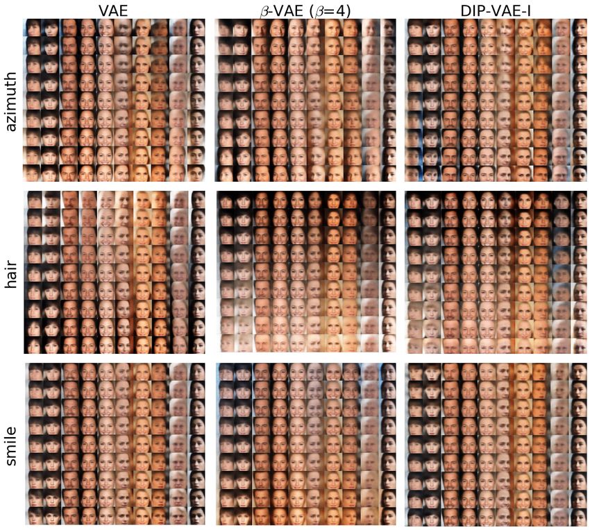
However, we observe in the decoder’s output for single latent traversals (varying a single latent
while keeping others fixed, shown in Fig. 3 and Fig. 4) that a high Z-diff score is not necessarily
a good indicator of disentanglement. Indeed, for 2D Shapes data, DIP-VAE-I has a higher Z-diff
score (98.7) and almost an order of magnitude lower reconstruction error than β-VAE for β = 60,
however comparing the latent traversals of β-VAE in Fig. 3 and DIP-VAE-I in Fig. 4 indicate a better
disentanglement for β-VAE for β = 60 (though at the cost of much worse reconstruction where
every generated sample looks like a hazy blob). On the other hand, we find the proposed SAP score
to be correlated well with the qualitative disentanglement seen in the latent traversal plots. This is
reflected in the higher SAP score of β-VAE for β = 60 than DIP-VAE-I. We also observe that for 2D
Shapes data, DIP-VAE-II gives a much better trade-off between disentanglement (measured by the
SAP score) and reconstruction error than both DIP-VAE-I and β-VAE, as shown quantitatively in
Fig. 1 and qualitatively in the latent traversal plots in Fig. 3. The reason is that DIP-VAE-I enforces
[Covp(x) [µφ (x)]]ii to be close to 1 and this may affect the disentanglement adversely by splitting a
generative factor across multiple latents for 2D Shapes where the generative factors are much less
than the latent dimension. For real datasets having lots of factors with complex generative processes,
such as CelebA, DIP-VAE-I is expected to work well which can be seen in Fig. 2 where DIP-AVE-I
yields a much lower reconstruction error with a higher SAP score (as well as higher Z-diff scores).
Binary attribute classification for CelebA. We also experiment with predicting the binary attribute
P from the inferred µφ (x). P
values for each test example in CelebA For each attribute k, we compute the
attribute vector wk = |xi :y1k =1| xi :yk =1 µφ (xi ) − |xi :y1k =0| xi :yk =0 µφ (xi ) from the training
i i i i
8Published as a conference paper at ICLR 2018
Figure 3: Qualitative results for disentanglement in 2D Shapes dataset (Matthey et al., 2017). SAP
scores, Z-diff scores and reconstruction errors for the methods (rows) can be read from Fig. 1.
9Published as a conference paper at ICLR 2018
Figure 4: Qualitative results for disentanglement in 2D Shapes dataset (Matthey et al., 2017) for
DIP-VAE-I (SAP score 0.1889).
set, and project the µφ (x) along these vectors. A bias is learned on these scalars (by minimizing
hinge loss) which is then used for classifying the test examples. Table 2 shows the results for the
attribute which show the highest change across various methods (most other attribute accuracies do
not change). The proposed DIP-VAE outperforms both VAE and β-VAE for most attributes. The
performance of β-VAE gets worse as β is increased further.
5 R ELATED W ORK
Adversarial autoencoder (Makhzani et al., 2015) also matches qφ (z) (which is referred as aggregated
posterior in their work) to the prior p(z). However, adversarial autoencoder does not have the
goal of minimizing
KL(qφ (z|x)||pθ (z|x))
which is the primary goal of variational inference. It
maximizes Ex Ez∼qφ (z|x) [log pθ (x|z)] −λ D(qφ (z)kp(z)), where D is the distance induced by
a discriminator that tries to classify z ∼ qφ (z) from z ∼ p(z) by optimizing a cross-entropy loss
(which induces JS-divergence as D). This can be contrasted with the objective in (4).
Invariance and Equivariance. Disentanglement is closely connected to invariance and equivariance
of representations. If R : x → z is a function that maps the observations to the feature representions,
equivariance (with respect to T ) implies that a primitive transformation T of the input results in
a corresponding transformation T 0 of the feature, i.e., R(T (x)) = T 0 (R(x)). Disentanglement
requires that T 0 acts only on a small subset of dimensions of R(x) (a sparse action). In this sense,
equivariance is a more general notion encompassing disentanglement as a special case, however this
special case carries additional benefits of interpretability, ease of transferrability, etc. Invariance is
also a special case of equivariance which requires T 0 to be identity for R to be invariant to the action
of T on the input observations. However, invariance can obtained more easily from disentangled
representations than from equivariant representations by simply marginalizing the appropriate subset
of dimensions. There exists a lot of prior work in the literature on equivariant and invariant feature
learning, mostly under the supervised setting which assumes the knowledge about the nature of input
transformations (e.g., rotations, translations, scaling for images, etc.) (Schmidt & Roth, 2012; Bruna
& Mallat, 2013; Anselmi et al., 2014; 2016; Cohen & Welling, 2016; Dieleman et al., 2016; Haasdonk
et al., 2005; Mroueh et al., 2015; Raj et al., 2017).
6 C ONCLUDING R EMARKS
We proposed a principled variational framework to infer disentangled latents from unlabeled ob-
servations. Unlike β-VAE, our variational objective does not have any conflict between the data
log-likelihood and the disentanglement of the inferred latents, which is reflected in the empirical
results. We also proposed the SAP disentanglement metric that is much better correlated with the
qualitative disentanglement seen in the latent traversals than the Z-diff score Higgins et al. (2017).
An interesting direction for future work is to take into account the sampling biases in the generative
process, both natural (e.g., sampling the female gender makes it unlikely to sample beard for face
images in CelebA) as well as artificial (e.g., a collection of face images that contain much more
10Published as a conference paper at ICLR 2018
smiling faces for males than females misleading us to believe p(gender,smile) 6= p(gender)p(smile)),
which makes the problem challenging and also somewhat less well defined (at least in the case
of natural biases). Effective use of disentangled representations for transfer learning is another
interesting direction for future work.
R EFERENCES
Fabio Anselmi, Joel Z Leibo, Lorenzo Rosasco, Jim Mutch, Andrea Tacchetti, and Tomaso Poggio.
Unsupervised learning of invariant representations in hierarchical architectures. arXiv preprint
arXiv:1311.4158, 2014.
Fabio Anselmi, Lorenzo Rosasco, and Tomaso Poggio. On invariance and selectivity in representation
learning. Information and Inference, 2016.
Martin Arjovsky and Léon Bottou. Towards principled methods for training generative adversarial
networks. In NIPS 2016 Workshop on Adversarial Training. In review for ICLR, volume 2016,
2017.
Martin Arjovsky, Soumith Chintala, and Léon Bottou. Wasserstein gan. arXiv preprint
arXiv:1701.07875, 2017.
Mathieu Aubry, Daniel Maturana, Alexei A Efros, Bryan C Russell, and Josef Sivic. Seeing 3d chairs:
exemplar part-based 2d-3d alignment using a large dataset of cad models. In Proceedings of the
IEEE conference on computer vision and pattern recognition, pp. 3762–3769, 2014.
Yoshua Bengio, Aaron Courville, and Pascal Vincent. Representation learning: A review and new
perspectives. IEEE transactions on pattern analysis and machine intelligence, 35(8):1798–1828,
2013.
David M Blei, Alp Kucukelbir, and Jon D McAuliffe. Variational inference: A review for statisticians.
Journal of the American Statistical Association, 2017.
Samuel R Bowman, Luke Vilnis, Oriol Vinyals, Andrew M Dai, Rafal Jozefowicz, and Samy Bengio.
Generating sentences from a continuous space. arXiv preprint arXiv:1511.06349, 2015.
Joan Bruna and Stephane Mallat. Invariant scattering convolution networks. IEEE Trans. Pattern
Anal. Mach. Intell., 2013.
Xi Chen, Yan Duan, Rein Houthooft, John Schulman, Ilya Sutskever, and Pieter Abbeel. Infogan:
Interpretable representation learning by information maximizing generative adversarial nets. In
Advances in Neural Information Processing Systems, pp. 2172–2180, 2016.
Brian Cheung, Jesse A Livezey, Arjun K Bansal, and Bruno A Olshausen. Discovering hidden factors
of variation in deep networks. arXiv preprint arXiv:1412.6583, 2014.
Taco Cohen and Max Welling. Learning the irreducible representations of commutative lie groups.
In International Conference on Machine Learning, pp. 1755–1763, 2014.
Taco Cohen and Max Welling. Group equivariant convolutional networks. In Proceedings of the 33rd
International Conference on Machine Learning, 2016.
Taco S Cohen and Max Welling. Transformation properties of learned visual representations. In
International Conference on Learning Representations, 2015.
Emily Denton and Vighnesh Birodkar. Unsupervised learning of disentangled representations from
video. arXiv preprint arXiv:1705.10915, 2017.
Guillaume Desjardins, Aaron Courville, and Yoshua Bengio. Disentangling factors of variation via
generative entangling. arXiv preprint arXiv:1210.5474, 2012.
Sander Dieleman, Jeffrey De Fauw, and Koray Kavukcuoglu. Exploiting cyclic symmetry in convolu-
tional neural networks. ICML, 2016.
11Published as a conference paper at ICLR 2018
Jeff Donahue, Philipp Krähenbühl, and Trevor Darrell. Adversarial feature learning. arXiv preprint
arXiv:1605.09782, 2016.
Alexey Dosovitskiy, Jost Tobias Springenberg, and Thomas Brox. Learning to generate chairs with
convolutional neural networks. In Proceedings of the IEEE Conference on Computer Vision and
Pattern Recognition, pp. 1538–1546, 2015.
Vincent Dumoulin, Ishmael Belghazi, Ben Poole, Alex Lamb, Martin Arjovsky, Olivier Mastropietro,
and Aaron Courville. Adversarially learned inference. arXiv preprint arXiv:1606.00704, 2016.
Gintare Karolina Dziugaite, Daniel M Roy, and Zoubin Ghahramani. Training generative neural net-
works via maximum mean discrepancy optimization. In Proceedings of the Thirty-First Conference
on Uncertainty in Artificial Intelligence, pp. 258–267. AUAI Press, 2015.
Marco Fraccaro, Simon Kamronn, Ulrich Paquet, and Ole Winther. A disentangled recognition and
nonlinear dynamics model for unsupervised learning. arXiv preprint arXiv:1710.05741, 2017.
Michael C Fu. Gradient estimation. Handbooks in operations research and management science, 13:
575–616, 2006.
Samuel Gershman and Noah Goodman. Amortized inference in probabilistic reasoning. In Proceed-
ings of the Cognitive Science Society, volume 36, 2014.
Ian Goodfellow, Jean Pouget-Abadie, Mehdi Mirza, Bing Xu, David Warde-Farley, Sherjil Ozair,
Aaron Courville, and Yoshua Bengio. Generative adversarial nets. In Advances in neural informa-
tion processing systems, pp. 2672–2680, 2014.
Ross Goroshin, Michael F Mathieu, and Yann LeCun. Learning to linearize under uncertainty. In
Advances in Neural Information Processing Systems, pp. 1234–1242, 2015.
Arthur Gretton, Karsten M Borgwardt, Malte J Rasch, Bernhard Schölkopf, and Alexander Smola. A
kernel two-sample test. Journal of Machine Learning Research, 13(Mar):723–773, 2012.
Bernard Haasdonk, A Vossen, and Hans Burkhardt. Invariance in kernel methods by haar-integration
kernels. In Scandinavian Conference on Image Analysis, pp. 841–851. Springer, 2005.
Irina Higgins, Loic Matthey, Arka Pal, Christopher Burgess, Xavier Glorot, Matthew Botvinick,
Shakir Mohamed, and Alexander Lerchner. beta-vae: Learning basic visual concepts with a
constrained variational framework. In International Conference on Learning Representations,
2017.
Geoffrey E Hinton, Alex Krizhevsky, and Sida D Wang. Transforming auto-encoders. In International
Conference on Artificial Neural Networks, pp. 44–51. Springer, 2011.
Matthew D Hoffman, David M Blei, Chong Wang, and John Paisley. Stochastic variational inference.
The Journal of Machine Learning Research, 14(1):1303–1347, 2013.
Xianxu Hou, Linlin Shen, Ke Sun, and Guoping Qiu. Deep feature consistent variational autoencoder.
In Applications of Computer Vision (WACV), 2017 IEEE Winter Conference on, pp. 1133–1141.
IEEE, 2017.
Wei-Ning Hsu, Yu Zhang, and James Glass. Unsupervised learning of disentangled latent representa-
tions from sequential data. In Advances in neural information processing systems, 2017.
Theofanis Karaletsos, Serge Belongie, and Gunnar Rätsch. Bayesian representation learning with
oracle constraints. arXiv preprint arXiv:1506.05011, 2015.
Diederik P Kingma and Max Welling. Auto-encoding variational bayes. arXiv preprint
arXiv:1312.6114, 2013.
Tejas D Kulkarni, William F Whitney, Pushmeet Kohli, and Josh Tenenbaum. Deep convolutional
inverse graphics network. In Advances in Neural Information Processing Systems, pp. 2539–2547,
2015.
12Published as a conference paper at ICLR 2018
Abhishek Kumar, Prasanna Sattigeri, and P Thomas Fletcher. Semi-supervised learning with GANs:
Manifold invariance with improved inference. In Advances in Neural Information Processing
Systems, 2017.
Brenden M Lake, Tomer D Ullman, Joshua B Tenenbaum, and Samuel J Gershman. Building
machines that learn and think like people. Behavioral and Brain Sciences, pp. 1–101, 2016.
Yujia Li, Kevin Swersky, and Rich Zemel. Generative moment matching networks. In Proceedings
of the 32nd International Conference on Machine Learning (ICML-15), pp. 1718–1727, 2015.
Ziwei Liu, Ping Luo, Xiaogang Wang, and Xiaoou Tang. Deep learning face attributes in the wild. In
Proceedings of the IEEE International Conference on Computer Vision, pp. 3730–3738, 2015.
Alireza Makhzani, Jonathon Shlens, Navdeep Jaitly, Ian Goodfellow, and Brendan Frey. Adversarial
autoencoders. arXiv preprint arXiv:1511.05644, 2015.
Michael F Mathieu, Junbo Jake Zhao, Junbo Zhao, Aditya Ramesh, Pablo Sprechmann, and Yann
LeCun. Disentangling factors of variation in deep representation using adversarial training. In
Advances in Neural Information Processing Systems, pp. 5040–5048, 2016.
Loic Matthey, Irina Higgins, Demis Hassabis, and Alexander Lerchner. dsprites: Disentanglement
testing sprites dataset. https://github.com/deepmind/dsprites-dataset/, 2017.
Yishu Miao, Lei Yu, and Phil Blunsom. Neural variational inference for text processing. In
International Conference on Machine Learning, pp. 1727–1736, 2016.
Youssef Mroueh, Stephen Voinea, and Tomaso A Poggio. Learning with group invariant features: A
kernel perspective. In Advances in Neural Information Processing Systems, pp. 1558–1566, 2015.
XuanLong Nguyen, Martin J Wainwright, and Michael I Jordan. Estimating divergence functionals
and the likelihood ratio by convex risk minimization. IEEE Transactions on Information Theory,
56(11):5847–5861, 2010.
Sebastian Nowozin, Botond Cseke, and Ryota Tomioka. f-gan: Training generative neural samplers
using variational divergence minimization. In Advances in Neural Information Processing Systems,
pp. 271–279, 2016.
Anant Raj, Abhishek Kumar, Youssef Mroueh, P Thomas Fletcher, and Bernhard Schlkopf. Local
group invariant representations via orbit embeddings. In AISTATS, 2017.
Scott Reed, Kihyuk Sohn, Yuting Zhang, and Honglak Lee. Learning to disentangle factors of
variation with manifold interaction. In International Conference on Machine Learning, pp. 1431–
1439, 2014.
Danilo Jimenez Rezende, Shakir Mohamed, and Daan Wierstra. Stochastic backpropagation and
approximate inference in deep generative models. arXiv preprint arXiv:1401.4082, 2014.
Karl Ridgeway. A survey of inductive biases for factorial representation-learning. arXiv preprint
arXiv:1612.05299, 2016.
Jurgen Schmidhuber. Learning factorial codes by predictability minimization. Neural computation, 4
(6):863–879, 1992.
Uwe Schmidt and Stefan Roth. Learning rotation-aware features: From invariant priors to equivariant
descriptors. In Computer Vision and Pattern Recognition (CVPR), 2012 IEEE Conference on,
2012.
N Siddharth, Brooks Paige, Van de Meent, Alban Desmaison, Frank Wood, Noah D Goodman,
Pushmeet Kohli, Philip HS Torr, et al. Learning disentangled representations with semi-supervised
deep generative models. arXiv preprint arXiv:1706.00400, 2017.
Bharath K Sriperumbudur, Kenji Fukumizu, Arthur Gretton, Bernhard Schölkopf, and Gert RG
Lanckriet. On integral probability metrics,\phi-divergences and binary classification. arXiv
preprint arXiv:0901.2698, 2009.
13Published as a conference paper at ICLR 2018
Andreas Stuhlmüller, Jacob Taylor, and Noah Goodman. Learning stochastic inverses. In Advances
in neural information processing systems, pp. 3048–3056, 2013.
Tim Van Erven and Peter Harremos. Rényi divergence and kullback-leibler divergence. IEEE
Transactions on Information Theory, 60(7):3797–3820, 2014.
William F Whitney, Michael Chang, Tejas Kulkarni, and Joshua B Tenenbaum. Understanding visual
concepts with continuation learning. arXiv preprint arXiv:1602.06822, 2016.
Jimei Yang, Scott E Reed, Ming-Hsuan Yang, and Honglak Lee. Weakly-supervised disentangling
with recurrent transformations for 3d view synthesis. In Advances in Neural Information Processing
Systems, pp. 1099–1107, 2015.
Shengjia Zhao, Jiaming Song, and Stefano Ermon. Towards deeper understanding of variational
autoencoding models. arXiv preprint arXiv:1702.08658, 2017.
14Published as a conference paper at ICLR 2018
Appendix
A L ATENT TRAVERSALS FOR 2D S HAPES AND C HAIRS DATASET
Figure 5: Qualitative results for disentanglement in CelebA dataset.
15Published as a conference paper at ICLR 2018
Figure 6: Qualitative results for disentanglement in Chairs dataset.
16You can also read