Playing Codenames with Language Graphs and Word Embeddings
←
→
Page content transcription
If your browser does not render page correctly, please read the page content below
Journal of Artificial Intelligence Research (2021)                     Submitted 00/00; published 00/00

                                                Playing Codenames with Language Graphs and Word
                                                                  Embeddings

                                         Divya Koyyalagunta*                                                      divyakoyy@gmail.com
                                         Anna Sun*                                                            anna.sun@alumni.duke.edu
                                         Rachel Lea Draelos                                                            rlb61@duke.edu
                                         Cynthia Rudin                                                             cynthia@cs.duke.edu
arXiv:2105.05885v1 [cs.CL] 12 May 2021

                                         Department of Computer Science
                                         Duke University
                                         Durham, NC 27708, USA
                                         *contributed equally

                                                                                              Abstract
                                                  Although board games and video games have been studied for decades in artificial
                                              intelligence research, challenging word games remain relatively unexplored. Word games
                                              are not as constrained as games like chess or poker. Instead, word game strategy is defined
                                              by the players’ understanding of the way words relate to each other. The word game
                                              Codenames provides a unique opportunity to investigate common sense understanding
                                              of relationships between words, an important open challenge. We propose an algorithm
                                              that can generate Codenames clues from the language graph BabelNet or from any of
                                              several embedding methods – word2vec, GloVe, fastText or BERT. We introduce a new
                                              scoring function that measures the quality of clues, and we propose a weighting term called
                                              DETECT that incorporates dictionary-based word representations and document frequency
                                              to improve clue selection. We develop BabelNet-Word Selection Framework (BabelNet-
                                              WSF) to improve BabelNet clue quality and overcome the computational barriers that
                                              previously prevented leveraging language graphs for Codenames. Extensive experiments
                                              with human evaluators demonstrate that our proposed innovations yield state-of-the-art
                                              performance, with up to 102.8% improvement in precision@2 in some cases. Overall, this
                                              work advances the formal study of word games and approaches for common sense language
                                              understanding.

                                         1. Introduction

                                         If you wanted to cue the words “piano” and “mouse,” but not “bison” or “tree” would you
                                         have immediately thought of the clue “keyboard”? If so, perhaps you are an expert at the
                                         game Codenames. This clue, however, was not provided by a human expert – rather, it was
                                         provided by an automated Codenames player that we introduce in this work.
                                            For decades, games have served as a valuable testbed for research in artificial intelligence
                                         (Yannakakis & Togelius, 2018). Deep neural networks have outperformed human experts in
                                         chess (Campbell, Hoane Jr, & Hsu, 2002), Go (Silver, Huang, Maddison, Guez, Sifre, et al.,
                                         2016), and StarCraft (Vinyals, Babuschkin, Czarnecki, Mathieu, Dudzik, et al., 2019). In
                                         comparison, progress in AI for word games is more limited. The study of word games
                                         has immense potential to facilitate deeper insight into how well models represent language,
                                         particularly common sense relationships between words.

                                         ©2021 AI Access Foundation. All rights reserved.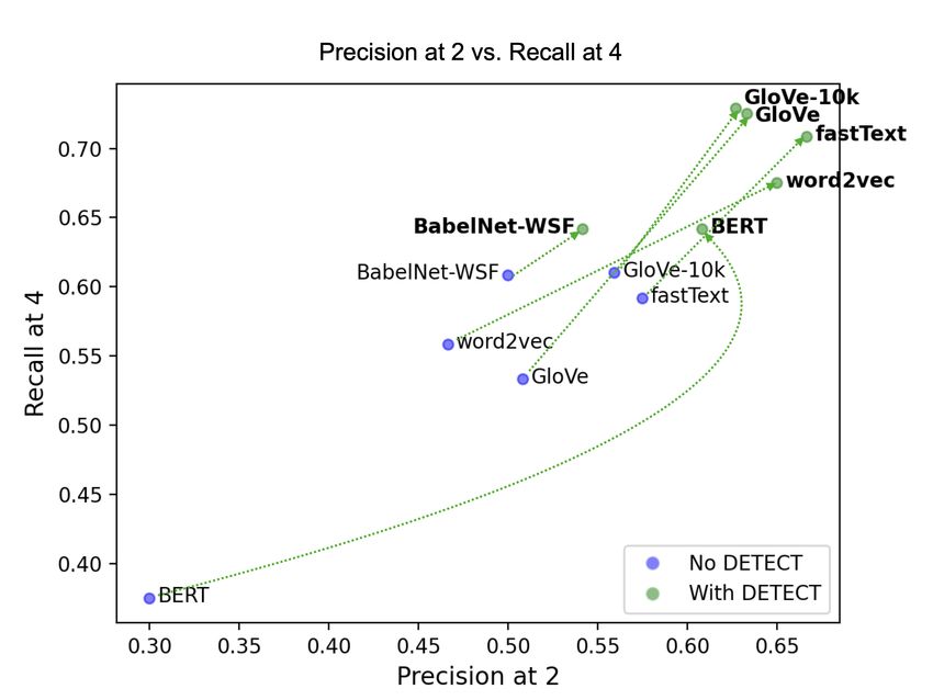
Koyyalagunta, Sun, Draelos, & Rudin

Figure 1: Example of a simplified version of a Codenames board. Blue words belong to
the blue team and red words to the red team. Only the clue-givers can see which words
belong to which teams. A clue-giver on the blue team generates clues to induce the blue
team guessers to pick blue words. The team that identifies all of their own words first wins.
In this figure, the table shows clues chosen for the blue team by applying our DETECT
algorithm, using various word representations. “Animals” is an example of a clue that is too
generic, as it also applies to the red words “calf” and “mammoth.” “Salmon” is a good clue
for the intended word “fish” but less likely to induce a guesser to choose the intended word
“bison” – however, “pirate” and “port” are the only other related words, which are both
blue and therefore will not result in a penalty. “Harbour” successfully indicates “pirate”
and “port” without applying to any red words, meaning it is a high-quality clue. Similarly,
“rock” connects to “diamond” and “cliff” without any close relationships to red words.

Figure 2: Clues chosen for board words by one of our algorithms using various word repre-
sentations.

    Codenames is a word game in which a clue-giver must analyze 25 board words and
choose a clue word that connects to as many of their own team’s words as possible, while
avoiding the opposing team’s words (Figure 1). Only the clue-giver knows which words
belong to their team, so it is critical that the clue-giver avoid selecting a clue that will
cause their team members to guess the opposing team’s words. Choosing quality clues
requires understanding complex semantic relationships between words, including linguistic
relationships such as syno-, anto-, hyper-, hypo- and meronymy, references to history and

                                             2
Playing Codenames with Language Graphs and Word Embeddings
popular culture, and polysemy (the multiple meanings associated with one word). For
example in Figure 2, the clue “keyboard” connecting the words “piano” and “mouse” uses
polysemy (a keyboard can refer to a musical keyboard or a computer keyboard), hyponymy
(a keyboard is-a piano), and context (a computer keyboard is generally accompanied by a
mouse). Thus, Codenames is distinct from other natural language processing tasks such as
word sense disambiguation (e.g., Iacobacci et al. (2016)) which focuses solely on polysemy,
machine translation (e.g., Devlin et al. (2014)) which focuses on cross-lingual understanding,
or part-of-speech tagging (e.g., Collobert et al. (2011)) which focuses on the grammatical
role of words in a sentence.
Previous work on Codenames has leveraged word embedding models as both clue-givers
and guessers, in order to evaluate performance based on how many times a model wins when
paired with another model (Kim, Ruzmaykin, Truong, & Summerville, 2019; Jaramillo,
Charity, Canaan, & Togelius, 2020). This performance evaluation measures how closely the
embedding spaces of two methods align, and does not indicate the actual clue quality as
judged by a human player. For example, the clue “duke” chosen for the board word “slug”
from word2vec results in a correct guess by a word2vec guesser, but would likely result in
a miss by a human guesser. Thus, when one word embedding method judges another, it
is possible for the clue-giver embedding method to obtain “high performance” in spite of
producing nonsensical clues. Instead of using computer simulations for our evaluations, we
conduct extensive experiments with Amazon Mechanical Turk to validate the performance
of our algorithms through human evaluation.
Previous work has been unable to leverage language graphs for Codenames due to com-
putational barriers. We introduce a new framework, BabelNet-WSF, that improves com-
putational performance by caching subgraphs and introducing constraints on the types of
graph traversals that are allowed. The constraints also improve clue quality by permitting
traversals only along paths for which the starting and ending node remain conceptually
connected to each other. Additionally, we introduce a method that extracts semantically
relevant single-word clues from BabelNet synsets, which are groupings of synonymous words
associated with a node in the graph. On the whole, BabelNet-WSF enables competitive
Codenames performance while remaining broadly applicable to other downstream tasks,
including word sense disambiguation (e.g., Navigli, Jurgens, and Vannella (2013)) and se-
mantic relatedness tasks (e.g., Navigli and Ponzetto (2012)).
In addition to our proposed methods for knowledge graphs, we introduce techniques
that improve Codenames performance for both word embedding-based and knowledge-based
methods. Most embedding methods rely on a word’s context to generate its vector represen-
tation. There are two main limitations to this context-based approach for the Codenames
task: (1) the resulting embeddings are capable of placing rare words (typically bad clues)
close to common words, and (2) important relationships such as meronymy and hypernymy
are difficult to capture in embedding methods. In the case of meronymy for example, parts
of things (e.g. “finger”) do not necessarily have the same context as the whole thing (e.g.
“hand”). To address these limitations, we propose DETECT, (DocumEnT frEquency +
diCT2vec), a scoring approach that combines document frequency, a weighting term that
favors common words over rare words, with an embedding of dictionary definitions. Dic-
tionary definitions more effectively capture meronymy, synonymy, and fundamental seman-
tic relationships. For the embedding of dictionary definitions, we use Dict2Vec (Tissier,
3Koyyalagunta, Sun, Draelos, & Rudin
Gravier, & Habrard, 2017), though our method can be used with other dictionary-based
embeddings. DETECT significantly improves clue quality, with an increase of up to 102.8%
precision@2 above baseline algorithms when evaluated by human players. Furthermore,
DETECT leads to universal improvement on Codenames across all four word embedding
methods (word2vec, GloVe, fastText, BERT) as well as an improvement on BabelNet-WSF.
The fact that our methods lead to improvement across all word representation methods
is significant, especially in the context of recent work that suggests different word represen-
tation methods may be best suited to different sub-tasks. For example, CBOW outperforms
GloVe on a Categorization task (clustering words into categories), but GloVe outperforms
CBOW on Selectional Preference (determining how typical it is for a noun to be the subject
or object of a verb) (Schnabel et al., 2015). DETECT is a promising metric to re-weight
word similarities in embedding space and in knowledge graphs anywhere that word repre-
sentations are used, such as comment analysis or recommendation engines.
This work shows promising results on a difficult word game task that involves many
layers of language understanding and human creativity. Because we have focused on hu-
man evaluation, we identified problem areas in which word representations fail to perform
well, and propose solutions that improve performance dramatically. Overall, our proposed
methods advance the formal study of word games and the evaluation of word embeddings
and language graphs in their ability to represent common sense language understanding.
2. Related Work
The closest related work to ours is that of Kim et al. (2019), who proposed an approach
for Codenames clue-giving that relies on word embeddings to select clues that are related
to board words. They evaluated the performance of word2vec and GloVe Codenames clue-
giver bots by pairing them with word2vec and GloVe guesser bots. Although this evaluation
approach is easy to run repeatedly over many trials, as it is purely simulation-based, the
evaluation is limited to how well the clue-givers and guessers “cooperate” with one another.
“Cooperation” measures how well GloVe and word2vec embedding representations of words
are aligned on similarity or dissimilarity of given words. To be more explicit, two methods
with different embeddings “cooperate well” if word embeddings that are relatively close
based on the clue-giver’s embeddings are also close based on the guesser’s embeddings, and
vice versa. As a result, it is clear that perfect performance (100% win percentage) comes
from pairing a clue-giver and a guesser who share the same embedding method. However,
this “cooperation” metric does not evaluate whether a clue given by a clue-giver is actually
a good clue – that is, a clue that would make sense to a human.
To address this limitation, in this paper, we evaluate Codenames clue-givers based on
human performance on the task of guessing correct words given a clue generated by an
algorithm.
Kim et al. (2019) also explored the use of knowledge graphs for Codenames clue-giving,
but ultimately did not consider knowledge-graph-based clue-givers in their final evaluation
due to poor qualitative performance and computational expense. In contrast, we propose
a method for an interpretable knowledge-graph-based clue-giver that performs competi-
tively with embedding-based approaches. The knowledge-graph-based method has a clear
advantage in interpretability over the embedding-based approaches.
4Playing Codenames with Language Graphs and Word Embeddings
In an extension of Kim et al. (2019), Jaramillo et al. (2020) compared the baseline
word2vec + GloVe word representations with versions using TF-IDF values, classes from
a naive Bayes classifier, or nearest neighbors of a GPT-2 Transformer representation of
the concatenated board words. Similar to Kim et al. (2019), they evaluated their methods
primarily by pairing clue-giver bots with guesser bots. They included an initial human
evaluation, where 10 games were played for both the baseline (word2vec + GloVe) and the
Transformer representations as clue-giver and guesser, but the human evaluation is limited
to only 40 games. Again, since evaluations from bots may not represent human judgments,
our human evaluation is more realistic and extensive, conducted through Amazon Mechan-
ical Turk with 1,440 total samples.
Another method (Zunjani & Olteteanu, 2019) proposes a formalization of the Code-
names task using a knowledge graph, but does not provide an implementation of their
proposed recursive traversal algorithm. We found that recursive traversal does not scale
to the computation required to run repeated evaluations of Codenames - for each blue
word, we must find each associated word w in the knowledge base that have Associationw,b
greater than some threshold t, and repeat this process every trial. In BabelNet, because
each word may be connected to tens or hundreds of other words, this becomes unscalable
when traversing more than one or two levels of edges. We propose an approach that scales
significantly better than naive recursive traversal by limiting paths through the graph to
those that yield high-quality clues.
Shen et al. (2018) also propose a simpler version of the Codenames task with human
evaluation. The experimental setup focuses on comparing different semantic association
metrics, including a knowledge-graph based metric. Their task differs from ours in two key
ways. First, each of their trials considers three candidate clues drawn from a vocabulary
of 100 words, whereas we consider candidate clues drawn from the larger vocabulary of all
English words. Second, their usage of ConceptNet is different from our usage of BabelNet
because they use vector representations derived from an ensemble of word2vec, GloVe, and
ConceptNet using retrofitting (Speer, Chin, & Havasi, 2017) whereas we leverage the graph
structure of BabelNet.
2.1 Other language games
Ashktorab et al. (2021) propose three different AI approaches for a word game similar
to Taboo, including a supervised model trained on Taboo card words, a reinforcement
learning model, and count-based model using a word evocation dataset. Their task, in
which an agent gives clues until a user guesses the secret word, is different from Codenames.
However, the datasets used in their models present interesting directions for future work in
the Codenames task. Ashktorab et al. (2021) propose three different AI approaches for a
word game similar to Taboo, including a supervised model trained on Taboo card words,
a reinforcement learning model, and count-based model using the Small World of Words
(De Deyne et al., 2019), a word evocation dataset. Their task, in which an agent gives
clues until a user guesses the secret word, is different from Codenames. However, the word
evocation dataset used in their count-based model could be leveraged for the Codenames
task since it represents word relatedness, and presents interesting directions for future work.
Another related task is the Taboo Challenge competition (Rovatsos, Gromann, & Bella,
5Koyyalagunta, Sun, Draelos, & Rudin
Figure 3: An overview of our proposed methods for improving Codenames performance. For
word embedding approaches, this involves pre-computing nearest neighbors for all board
words (e.g., gold, lemon, diamond, calf, flute and ice as shown above). To pre-compute
nearest neighbors using BabelNet-WSF, we query BabelNet for every board word, and then
construct the semantically relevant subgraph connected to that board word (described in
Section 3.2.2). We then cache the subgraphs for later use (see Section 3.2.1), and extract
single-word clues from BabelNet synsets (see Section 3.2.3). In Section 3.4, we describe
how we get single word embeddings from a contextual embedding based method such as
BERT. Once candidate clues are produced by either a word embedding or BabelNet-WSF,
we use the ClueGiver algorithm described in Section 3.1 and apply our DETECT weighting
term to choose the best clue for that board (see Section 3.3).
6Playing Codenames with Language Graphs and Word Embeddings
2018), where AI systems must guess a city based on clues crowdsourced from humans. In
this task, the AI system acts as the guesser, rather than the clue giver.
Other work in language games that are similar to Codenames include the Text-Based
Adventure competition (Atkinson et al., 2019), which evaluates agents in text-based adven-
ture games, Xu and Kemp (2010), which models a task in which a speaker gives a one-word
clue to a listener with the goal of guessing a target word, and Thawani, Srivastava, and
Singh (2019), which proposes a task to evaluate embeddings based on human associations.
2.2 Quantifying Semantic Relatedness from WordNet
There is a body of previous work that proposes methods to quantify semantic relatedness in
a knowledge graph beyond simply counting the number of edges between two nodes. Hirst,
St-Onge, et al. (1998) developed a ranking of relationships into three groups, extra-strong,
strong, and medium-strong, where only medium-strong includes a numeric score based on
path length and path type; in our work we use numeric scores for all word comparisons
and do not separate into 3 categories. Budanitsky and Hirst (2006) evaluated different
techniques for the quantification of semantic relatedness for WordNet, but most techniques
used noun-only versions of WordNet, whereas we consider all parts of speech including
nouns, verbs, and adjectives. Furthermore, 4 of their 5 techniques restrict to hyponym
relationships whereas we consider multiple relationship types. The proposed PageRank
technique of Agirre et al. (2009) could be applied to BabelNet and is an interesting direction
for future work.
3. Methods
Codenames is a word-based, multiplayer board game illustrated in Figure 1. The board
consists of a total of 2N words, divided equally into the blue team’s words B = {bn }N n=1 and
the red team’s words R = {rn }N n=1 . Only the clue-giver knows which words are assigned to
which teams. A clue-giver provides a clue, and a guesser on their team selects a subset of
board words related to that clue. The team that guesses all of their own words first wins.
In this paper we focus on the task of clue-giving. The clue-giving task is the most
interesting, since the clue-giver needs to search the space of all possible words to identify
suitable clues, and then rank the clues to select the best one. A blue clue-giver must
generate a clue c that is conceptually closest to one subset (here, a pair) of blue words from
the set of all possible blue word pairs I ∈ B 2 . The clue c must also be sufficiently far from
all red words R. Note that in the original Codenames game, a clue-giver can produce a
clue corresponding to an arbitrary number of blue words from I ∈ B m for any m ≤ N , but
for more consistent evaluation we calculate performance on the clue-giving task considering
m = 2 only. Our proposed innovations apply for arbitrary m.
Figure 3 provides an overview of our proposed methods. In Section 3.1, we describe
the baseline algorithm for choosing and ranking clues. Section 3.2 details BabelNet-WSF,
our method for querying the very large BabelNet graph and multiple techniques to improve
the quality of the returned clues. In Section 3.3 we propose the DETECT algorithm which
leverages document frequency and dictionary embeddings to universally improve Codenames
performance across embedding and graph-based clue-givers. Finally, Section 3.5 explains
the extensive human evaluation experiments conducted through Amazon Mechanical Turk.
7Koyyalagunta, Sun, Draelos, & Rudin
All of our code for these proposed methods is available for public use.1
3.1 ClueGiver: a baseline algorithm that produces clues
We propose ClueGiver, an algorithm that gives clues on the basis of a measurement of word
similarity s(w1 , w2 ).
First, we define s(w1 , w2 ) for word-embedding-based and knowledge-graph-based ap-
proaches. For word embeddings, the word similarity s(w1 , w2 ) is defined as 1 minus the
cosine distance between the word embeddings, i.e. 1 − cos(f (w1 ), f (w2 )), where f is the
embedding function. When measuring word similarity with a knowledge graph method such
as BabelNet-WSF, the word similarity s(w1 , w2 ) is defined as the inverse of the number of
edges along the path between the graph node for word w1 and the graph node for word w2 ,
1
i.e. h(w1 ,w 2 )+1
, where h is a function that gives the number of edges along the shortest path
between w1 and w2 .
ClueGiver has two steps. To choose a clue for the blue team, we first calculate the T
nearest neighbors of each blue word in B = {bn }N n=1 . We go through each subset I ∈ B
m
and add the union of the nearest neighbors for every blue word b ∈ I to a set of candidate
clues C̃ = {c̃tn }t=1..T ;n=1..N . The subset I represents the set of intended words that are
meant to match the candidate clue. Every subset of B of size m is therefore considered as
a candidate set of intended words. Next, we score each candidate clue c̃ using the following
scoring function g(·) which produces a large positive value for good clues and a lower value
for bad clues (and thus should be maximized):
!
X
g(c̃, I) = λB s(c̃, b) − λR max s(c̃, r) (1)
r∈R
b∈I
The final chosen clue c is the candidate clue with the highest score.PA candidate clue c̃
will have a high score if it is closest to the subset I (thus making λB b∈I s(c̃, b) as large
as possible), while remaining as far away as possible from all the red words. The expression
maxr∈R s(c̃, r) means that we calculate the highest similarity between the red words and
our candidate clue c̃, which corresponds to the red word closest to c̃. If c̃ is a good clue for
the blue team, then even this closest red word is far away from the candidate clue, with
a small positive value of s(c̃, r). In the case that there is no overlap between the nearest
neighbors of the blue words, the algorithm will choose a clue for one word. This happened
extremely rarely when computing 500 nearest neighbors for each board word. The choices
of λB and λR determine the relative importance of each part of the scoring function, i.e.,
whether we should prioritize clues that are close to blue words or prioritize clues that are
far from red words. We found λB = 1 and λR = 0.5 to be effective values empirically across
all word representations. None of the human experiments used the same data that was
used to set these parameters. The Codenames boards used to tune the parameters were
randomly sampled from the total of 208
20 = 3.68e+27 Codenames boards (208 being the
possible board words, and 20 being the board size). The Codenames boards used for human
evaluation on AMT were different boards, randomly sampled from all possible boards with
1
each having probability 3.68e+27 .
1. https://github.com/divyakoyy/codenames
8Playing Codenames with Language Graphs and Word Embeddings
Comparison to the scoring function of Kim et al. (2019) In our experiments,
we compare our scoring function g(·) with the following scoring function proposed by Kim
et al. (2019). The term λT is configurable to limit how aggressive the clue-giver is:
(
minb∈I s(c̃, b), if minb∈I s(c̃, b) > λT and minb∈I s(c̃, b) > maxr∈R s(c̃, r)
gkim (c̃, I) =
0, otherwise
(2)
The main difference between gkim and our proposed scoring function g is that our scoring
function g incorporates a penalty to the score based on the similarity of the closest red word,
while gkim enforces the constraint that the similarity between the clue and the furthest blue
word must be greater than the similarity to the closest red word. In addition, gkim enforces
that the similarity between the furthest blue word and the clue is greater than the threshold
λT . Notably, gkim would give equal scores (assuming that blue word distances are equal)
to clue words that do not violate the constraint, even if one was much closer to a red word
than the other, whereas g applies a soft penalization to red words.
3.2 BabelNet-WSF: Solving Codenames clue-giving with the BabelNet
knowledge graph
As discussed previously, knowledge graphs have not been successfully used to play Co-
denames in prior work. In this section we propose BabelNet-WSF, which includes three
innovations to enable high-performance use of the BabelNet knowledge graph for the Code-
names clue-giving task, including (1) a method for constructing a nearest neighbor BabelNet
subgraph relevant to a particular Codenames board, (2) constraints that filter the nearest
neighbors to improve candidate clue quality, and (3) an approach to select a good single
word clue from the set of synonymous phrases associated with a particular node.
3.2.1 Constructing Subgraphs of BabelNet to Identify Nearest Neighbors
In order to choose a clue using the scoring function defined in the previous section, it is
necessary to identify the nearest neighbors of the board words. When solving Codenames
with a knowledge graph like BabelNet, the graph connectivity defines the nearest neighbors.
We define the “nearest neighbors” of an origin node as all nodes within 3 edges of the
origin node. The challenge arises because the full BabelNet 4.0.1 graph is 29 gigabytes,
so recursively traversing it to identify nearest neighbors is computationally prohibitive as
noted by Kim et al. (2019).
We propose three steps to enable fast nearest neighbors identification from BabelNet for
a particular Codenames board. First, we restrict the relationship edges that are added to
the subgraph. Every edge in the BabelNet graph indicates a particular type of relationship
(e.g. is-a). For each node in the graph representing a board word, we obtain all outgoing
edges for the first edge, but for edges beyond that, we only recursively traverse edges that
are in the hypernym relationship group, as discussed in Section 3.2.2.
Second, we exclude edges that were automatically generated, because we found these to
be of poor quality for the Codenames task. Finally, we cache the nearest neighbor results
for each board word, in order to reuse these results for future boards. This caching step
9Koyyalagunta, Sun, Draelos, & Rudin
is important due to a daily limit in querying the BabelNet API. Appendix Algorithm 2
details the overall process for obtaining nearest neighbors from BabelNet.
3.2.2 Filtering Nearest Neighbors for BabelNet
Once a nearest neighbor graph is constructed, we apply two filtering steps on the edges in
order to retain only the highest-quality nearest neighbors, and thereby improve the selected
clues.
Hypernym edge constraint beyond the first edge. The first filtering step is to only allow
hypernym relationships (is-a or subclass-of) beyond the first edge. The motivation be-
hind this constraint is that traversing the graph using randomly chosen relationship types
leads to “nearest neighbors” which are not very related to the origin node. However, us-
ing only hypernym relationship types is too restrictive, since exploiting different kinds of
relationships is critical in order to perform well at Codenames clue-giving. We found that
allowing the first edge to be any relationship type, but restricting all subsequent edges
to be a hypernym relationship type maintained diversity of clues while usually preserving
conceptual relatedness of the origin node and (possibly distant) neighbor node. Table 1
illustrates the improvement in nearest neighbor quality that this constraint yields.
HAS - PART
passes constraint needle −−−−−−→ point
HAS - PART HAS - KIND
fails constraint needle −−−−−−→ point −−−−−−→ spearhead
IS - A IS - A
passes constraint litter −−→ trash −−→ waste
IS - A HAS - KIND
fails constraint litter −−→ trash −−−−−−→ scrap metal
IS - A IS - A
passes constraint mouse −−→ pointing device −−→ input device
IS - A HAS - KIND
fails constraint mouse −−→ pointing device −−−−−−→ light gun
Table 1: Examples of hypernym edge constraint beyond the first edge. Hypernym relation-
ships are is-a or subclass-of. Words in red failed the constraint and are filtered out of
the graph.
Same-type edge constraint. The second constraint restricts all edges after the first edge
to be the same relationship type. In combination with the hypernym constraint, that means
a traversal after the first edge of is-a/is-a/is-a is allowed, a traversal after the first edge of
subclass-of/subclass-of/subclass-of is allowed, but any traversal after the first edge
randomly combining is-a and subclass-of is forbidden. We found that this additional
stringency improved the relevance of retrieved nearest neighbors. Examples are shown in
Table 2.
3.2.3 Selecting a good single-word clue from a multi-word synset
Once the nearest neighbors have been filtered, a final clue must be selected. In the Co-
denames task, the clue must consist only of a single word. However, each node of the
10Playing Codenames with Language Graphs and Word Embeddings
IS - A IS - A IS - A
passes constraint litter −−→ animal group −−→ biological group −−→ group
IS - A SUBCLASS - OF
passes constraint litter −−→ animal group −−−−−−−−→ fauna
IS - A SUBCLASS - OF IS - A
fails constraint litter −−→ animal group −−−−−−−−→ fauna −−→ aggregation
GLOSS - RELATED IS - A IS - A
passes constraint moon −−−−−−−−−−→ planet −−→ celestial body −−→ natural object
GLOSS - RELATED SUBCLASS - OF IS - A
fails constraint moon −−−−−−−−−−→ planet −−−−−−−−→ planemo −−→ object
GLOSS - RELATED IS - A IS - A
passes constraint figure −−−−−−−−−−→ diagram −−→ drawing −−→ representation
GLOSS - RELATED SUBCLASS - OF IS - A
fails constraint figure −−−−−−−−−−→ diagram −−−−−−−−→ graphics −−→ visual communication
Table 2: Examples of same-type edge constraint on edges after the first edge.
BabelNet graph is a synset, which is a group of related concepts organized as a “main sense
label” with “other sense labels.” To add to the complexity, each label can be one or more
words. For example from Table 3, the synset with the definition “material used to provide
a bed for animals” has a main sense label of “bedding,” and other sense labels “litter” and
“bedding material.” The synset with the main sense label “creative work” has other sense
labels “artwork,” “work,” and “work of art.” It is not immediately obvious how to extract
a good-quality single word clue from a synset.
Main sense label Definition Other labels
Material used to provide a bed for
bedding litter, bedding material
animals
bedclothes, bed cloth-
bedding Coverings that are used on a bed
ing
A musical instrument in which
string instrument,
stringed instrument taut strings provide the source of
chordophone
sound
A creative work is a manifesta-
tion of creative effort including fine creative work, artwork,
creative work
artwork, writing, filmmaking, and work, work of art
musical composition
Table 3: Examples of synsets with multi-word labels
Selecting a single word at random from a synset is not effective. For example “work” on
its own is not an ideal choice for “creative work” and “material” is not an ideal choice for
“bedding material.” We develop a scoring system to select the best possible single word clue
from a synset. First, we keep only single words that belong to the intersection of the nearest
neighbors of two board words. Taking a simplified example from Figure 3 (bottom), for the
board words “gold,” having neighbor synset with labels {“shades of yellow,” “variations of
11Koyyalagunta, Sun, Draelos, & Rudin
yellow”}, and “lemon,” having neighbor synset with labels {“yellow,” “yellowness,” “color
yellow”}, the word “yellow” is kept.
We also apply weights (which are parameters of our method) on each of the words
comprising the synset labels. The weights on these words are denoted by w1 , w2 , w3 , and
w4 where w1 ≤ w2 ≤ w3 ≤ w4 , and they are assigned based on the type of synset label and
whether the label has multiple words, as shown in Table 4. The number of edges h(c̃, w) is
multiplied by the weight; thus a label type with a lower weight, such as main-sense single
word, is desirable. Empirically, we found that the values w1 = 1, w2 = 1.1, w3 = 1.1, w4 =
1.2 to be effective. Appendix Algorithm 1 details the process for obtaining single-word
clues and their corresponding weights.
label type single- or multi- word weight
main sense single w1
main sense multi w2
other sense single w3
other sense multi w4
Table 4: Weights applied to labels taken from BabelNet depend on whether the label is
a main sense or other sense label (this distinction is provided by BabelNet), and whether
that label is composed of one or more words.
3.2.4 Example BabelNet-WSF Clue
The combination of the three aforementioned innovations enables selection of high-quality
clues from BabelNet, as exemplified in Figure 4.
musical
L HA
BE S-
LA
LA
S- BE
HA L
scale, musical scale composition, musical composition
bn:00056469n bn:17306106n
IS - A
opera
bn:00059107n
Figure 4: Sub-graph of BabelNet showing how the clue “musical” was chosen for the board
words “scale” and “opera” using BabelNet-WSF. The has-label edges are not real edges
in BabelNet, but rather single word labels that we extract using the single-word clue ap-
proach described in Section 3.2.3. Synsets from BabelNet are annotated with their ID from
BabelNet 4.0.1 as bn:synset-id.
12Playing Codenames with Language Graphs and Word Embeddings
3.3 DETECT for Improving Clue Quality
The previous sections focused on obtaining good clues from BabelNet. In this section, we
describe a method called DETECT that improves the quality of clues for both BabelNet-
WSF and word embedding-based methods. We originally developed DETECT to address
deficiencies in clues produced by word embedding-based methods, and then discovered that
DETECT also improved BabelNet-WSF clues. In our experiments, we show results of word
embedding and BabelNet-WSF methods with and without DETECT.
We identified three deficiencies in the clues chosen via word embeddings: (1) obscure
clues, (2) overly generic clues, and (3) lack of clues exploiting many common sense word
relationships. Table 5 provides real examples of clues that suffer from deficiencies (1) and
(2). Obscure clues are not necessarily “incorrect” in the way they connect two words: for
example the word “djedkare” in Table 5 refers to the name of the ruler of Egypt in the 25th
century B.C., and therefore correctly connects the words “egypt” and “king.” However this
clue does not reflect the average person’s knowledge of the English language and is likely to
yield random guesses if presented to a human player. Overly generic clues, in contrast, are
more likely to match too many board words. For example “artifact” in Table 5 connects
“key” and “pipe,” but also matches other red words on the board for that trial, such as
“crown” and “racket.”
Clue Intended Words to Match Clue
aether jupiter, vacuum
djedkare egypt, king
machine key, crown
artifact key, pipe
Table 5: Examples of obscure and generic clues. Obscure clues include “aether,” which
in ancient and medieval science is a material that fills the region of the universe above
the terrestrial sphere, and “djedkare” which is the name of the ruler of Egypt in the 25th
century B.C. Overly generic clues include “machine” and “artifact” which often apply to
many board words.
To address all three issues in clue quality, we added a scoring metric, DETECT, to our
scoring function g(·). DETECT includes two parts, a function F REQ(w) that uses docu-
ment frequency to exclude too-rare and too-common words, and a function DICT (w1 , w2 )
that encourages clues relying on common sense word relationships.
Leveraging document frequency with F REQ. In order to penalize overly rare as well as
overly generic tokens, we leverage the document frequency fw of a word, which indicates
the count of documents in which word w is found in a cleaned subset of Wikipedia. We
calculate F REQ(w) as:
(
1
when df1w ≥ α
F REQ(w) = − dfw (3)
1 when df1w < α.
F REQ(w) penalizes rare words more and common words less, unless a word is so com-
mon that the inverse function of its document frequency is lower than a value α, which is
13Koyyalagunta, Sun, Draelos, & Rudin
Figure 5: FREQ is a function of document frequency that is used to penalize rare words more
and common words less unless the word is so common that it is not useful as a clue word.
α was chosen by picking an upper bound document frequency and validating empirically
across clue-giving algorithms. Note that α = 1/1, 667 was calculated on a sample of 1,701
cleaned documents from (Mahoney, 2020).
an algorithm parameter. α was chosen empirically based on the distribution of document
frequencies in a cleaned subset of the Wikipedia corpus as shown in Figure 5, together
with the clues produced across all algorithms. α represents the upper bound document
frequency at which point a word is considered too common to be useful as a clue word.
Jaramillo et al. (2020) used TF-IDF as a standalone baseline method, whereas in this work
F REQ is a term which is part of the full scoring function.
In principle, Equation 1 should filter out overly generic clues that match red words
via the penalty we apply to red words. However we found that in practice, performance
improved by removing common words with the F REQ component of DETECT. This is
because of a limitation of BabelNet, in which the number of edges connecting a common
word to all of its children is highly variable (e.g. the number of edges between “object” and
“apple” is 4, vs. the number of edges between “object” and “cash” is 1).
Leveraging dictionary embeddings with DICT . Since most embedding methods rely
on a word’s context to generate its vector representation, they do not always encode im-
portant relationships such as meronymy and hypernymy. Dict2Vec (Tissier et al., 2017)
addresses this issue by computing vector representations of words using dictionary defini-
tions. Dict2Vec also identifies strong pairs of words as words that appear in each other’s
dictionary definition – for example, “car” might appear in the definition of “vehicle” and
vice versa, making “car”/“vehicle” a strong pair. Synonymy, hypernymy, hyponymy and
meronymy are all relationships captured in dictionary definitions and relationships that con-
tribute to high quality clues, so incorporating Dict2Vec into our scoring function allowed
us to more heavily weight clues that are semantically related in ways that context alone
cannot capture.
We define DICT (w1 , w2 ) as the cosine distance between the Dict2Vec word embeddings
for two words w1 and w2 .
14Playing Codenames with Language Graphs and Word Embeddings
The DETECT score. Both term relevance F REQ(w) and dictionary relevance DICT (w1 , w2 )
are incorporated into a new weighting term, DETECT:
X
DET ECT (c̃) = λF F REQ(c̃) + λD 1 − DICT (c̃, b) − max 1 − DICT (c̃, r) . (4)
r∈R
b∈I
A candidate clue c̃ will have a high value for DET ECT (c̃) if it is a more common word
(without being so common that it falls above α in Equation 3), and is close to as many
of
P the intended blue words as possible in the Dict2Vec embedding space (therefore making
b∈I 1 − DICT (c̃, b) as large as possible) while remaining as far as possible from red words.
DET ECT (c̃) is added to the scoring function g(·) of Equation 1 and gkim (·) of Equation
2 to re-weight candidate clues. We found λF = 2, λD = 1 for GloVe filtered on the top 10k
English words, and λD = 2 for all other representations, to be most effective empirically.
The word embeddings (word2vec, GloVe, fastText, BERT) were obtained from publicly
available collections of pre-trained vectors based on large corpora such as Wikipedia or
Google News. The word2vec, GloVe, and fastText vectors were obtained from the gensim
library (Řehůřek & Sojka, 2010), and BERT contextualized embeddings were obtained from
a pre-trained BERT model (bert 12 768 12, book corpus wiki en uncased) made available
in the GluonNLP package (Guo et al., 2020). DETECT leverages additional data sources
summarized in different ways to improve clue choosing. The Dict2Vec component of DE-
TECT uses dictionary definitions from Cambridge, Oxford Collins, and dictionary.com, and
an embedding method to summarize this data. The F REQ(w) component of DETECT
uses a cleaned subset of Wikipedia (Mahoney, 2020) and the F REQ(w) score to summarize
this data.
3.4 Using Contextual Embeddings
This section describes our final methodological contribution to improve Codenames clue-
giving: how to produce a clue using a contextual embedding method. In “classical” word
embedding methods such as GloVe (Pennington, Socher, & Manning, 2014) and word2vec
(Mikolov, Sutskever, Chen, Corrado, & Dean, 2013), each word is associated with only
one vector representation, so the Codenames scoring function in Equation 1 can be com-
puted directly. However, contextual embedding methods like BERT (Devlin, Chang, Lee, &
Toutanova, 2019) only produce a representation for a word in context. Therefore the word
“running” in the following sentences, “She was running to catch the bus,” and “She was
running for president,” are captured in their respective contexts. In order to compute the
Codenames scoring function using BERT embeddings, we averaged over different contexts
to produce a single embedding for each word. Specifically, we extracted contextualized em-
beddings from a pre-trained BERT model (bert 12 768 12, book corpus wiki en uncased),
made available by the GluonNLP package (Guo et al., 2020), using a cleaned subset of
English Wikipedia 2006 (Mahoney, 2020).
Then we defined a word’s BERT embedding as the average over that word’s contextual
embeddings. An approximate nearest neighbor graph was produced from the final embed-
dings using the Annoy library.2 Averaging allowed us to reduce noise caused by outlier
2. https://github.com/spotify/annoy
15Koyyalagunta, Sun, Draelos, & Rudin
contextual embeddings of a word, but in the future we could also experiment with clus-
tering of contextual embeddings and using those clusters to construct a nearest neighbor
graph.
3.5 Human Evaluation of Clue-Giving Performance
We use Amazon Mechanical Turk (AMT) for human evaluation of Codenames clue-giving
algorithms.
3.5.1 General performance comparison and efficacy of DETECT
We compare five Codenames clue-giving algorithms, based on our proposed scoring function
g(·) (Equation 1): (1) BabelNet-WSF, (2) word2vec (Mikolov et al., 2013), (3) GloVe
(Pennington et al., 2014), (4) GloVe-10k (filtering for the 10k most common words), (5)
fastText (Bojanowski et al., 2017), and (6) BERT (Devlin et al., 2019). Table 6 summarizes
all methods we used in our experiments, including baseline methods from Kim et al. (2019),
along with all of our new proposed methods and variations on those methods. The symbol
“ ” indicates something novel to the paper, whether it is a new use of a method (first
column), a new representation of words (second column), or uses our new ranking method
for clues (third column). This table includes the 3 baselines used in Kim et al. (2019), as well
as 9 new methods proposed in the paper. In our experiments, we evaluate each algorithm
with and without DETECT (Section 3.3), and with our scoring function and the Kim
et al. (2019) scoring function, for a total of 24 configurations. BabelNet-WSF includes the
innovations described in Section 3.2. BERT includes the innovations of Section 3.4.
To compare the algorithms, 60 unique Codenames boards of 20 words each were com-
putationally generated from a list of 208 words obtained from the official Codenames cards.
We used words from the official Codenames cards because these words were carefully se-
lected by the game designers to have interesting, inter-related multiple meanings, and as
such these words are an integral part of the game definition.
For a given Codenames board, each algorithm was asked to output the best clue and
the two words intended to match the clue. These two words are the blue words that the
algorithm based a particular clue on, which a human guesser is intended to select.
For human evaluation, United-States-based AMT workers with a high approval rate
(≥ 98%) on previous AMT tasks were asked to look at a full board of 20 words and 1 clue
word, and rank the top four board words matching the given clue. The user was required
to fill in Ranks 1 and 2, because the algorithm always intended 2 words to be selected.
Ranks 3 and 4 were optional for the user to fill in; the AMT worker could specify “no
more related words” for these ranks. Ranks 3 and 4 were included to distinguish between
situations where the algorithm produced a wholly irrelevant clue (such that the worker
could not guess the intended words even if given 4 slots) and a sub-optimal clue (such that
the worker could guess intended words in Ranks 3 or 4, but not Ranks 1 or 2). The AMT
workers had no knowledge of the underlying algorithm and no knowledge of the algorithm’s
“intended words.” A high-performing algorithm chooses such good quality clues that the
AMT workers correctly guess the intended words and place them in Ranks 1 and 2.
16Playing Codenames with Language Graphs and Word Embeddings
Word new use new use new knowledge new ranking
Representation in Codenames in Codenames graph method method
gkim (·) g(·) in Codenames
BabelNet-WSF no
BabelNet-
WSF+DETECT
BERT no no
BERT+DETECT no
fastText no no
fastText+DETECT no
GloVe no no
GloVe+DETECT no
GloVe-10k no no no
GloVe-
no
10k+DETECT
word2vec no no
word2vec+DETECT no
Table 6: A summary of all methods from our experiments, both baseline methods from Kim
et al. (2019) as well as new proposed methods and the variations on those methods. The
first column indicates whether an algorithm is a new method for Codenames using gkim (·)
scoring function, the second column indicates whether it is a new method for Codenames
using g(·) scoring function, the third column indicates whether a new knowledge graph
method is used, and the fourth column indicates the use of a new method for ranking clues.
3.5.2 Comparison with Kim et al. (2019)
In order to compare with the work of Kim et al. (2019), we also evaluated the performance of
each algorithm using their scoring function gkim (·) (Equation 2), using the same set of Co-
denames boards. In the original formulation of the Kim et al. (2019) scoring function shown
in Equation 2, the constraints minb∈I s(c̃, b) > λT and minb∈I s(c̃, b) > maxr∈R s(c̃, r) were
used. Since we evaluate performance on the clue-giving task considering m = 2 for consis-
tency of evaluation across all algorithms, this constraint was relaxed if there were no clue
words passing those constraints for m = 2 blue words.
In addition, Kim et al. (2019) restricts to the top 10k common English words. We
tested this using the GloVe model filtered on the top 10k common words, and refer to this
as GloVe-10k in our reported results.
3.5.3 Performance metrics
Each trial from Amazon Mechanical Turk provided the 2 to 4 board words (ranked) that the
AMT worker selected as most related to the given clue word. To quantify the performance
of different algorithms, we calculated precision@2 and recall@4. Precision@2 measures the
number of correct words that an AMT worker guessed in the first 2 ranks, where correct
17Koyyalagunta, Sun, Draelos, & Rudin
words are the intended words that the algorithm meant the worker to select for a given
clue. Recall@4 measures the number of correct words chosen in the first 4 ranks.
4. Results
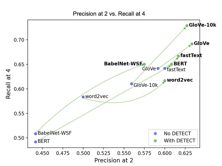
Figure 6: Precision@2 (for the 2 intended words chosen by the algorithm for a clue) vs.
Recall@4 (for the 4 words that guessers could answer) from Amazon Mechanical Turk
results using our proposed scoring function g(·).
Results from the different algorithms with our scoring function are shown in Figure 6,
while results for the different algorithms with the Kim et al. (2019) scoring function are
shown in Figure 7. Additional results from the AMT evaluation are reported in Appendix
A. The results are summarized as follows.
• Some of our methods surpass state-of-the-art performance for the Codenames clue-
giving task. The best-performing algorithm for precision@2 across both scoring func-
tions is fastText+DETECT, with 66.67% precision@2. fastText+DETECT out-
performs the prior state-of-the-art by Kim et al. (2019) using glove-10k,
which has precision 55.93% as shown in Figure 7.
• Our proposed DETECT algorithm leads to universal improvement across
all word representations with a median percent improvement of 18.0% for preci-
sion@2. DETECT also leads to improvement across both scoring functions, with a
18Playing Codenames with Language Graphs and Word Embeddings
Figure 7: Precision@2 (for the 2 intended words chosen by the algorithm for a clue) vs.
Recall@4 (for the 4 words that guessers could answer) from Amazon Mechanical Turk
results using the Kim et al. (2019) scoring function.
median 16.1% improvement for our scoring function and even higher median improve-
ment of 20.3% for the Kim et al. (2019) scoring function. For BERT, the advantage
of using DETECT is most substantial, with a 102.8% improvement in precision@2.
• When DETECT is used, our scoring function leads to better performance for BabelNet-
WSF, while the Kim et al. (2019) scoring function leads to better performance for
word2vec and fastText, and both performed equally on GloVe, GloVe-10k, and BERT
(precision@2). Thus, neither scoring function is definitively superior. However, since
BabelNet-WSF is more interpretable and easier to troubleshoot than the word em-
bedding methods, we suspect that our scoring function (which performs better on
BabelNet-WSF) might be more useful in settings where one might want to engineer
better performance for the system.
• We report the first successful use of a knowledge graph to solve the Code-
names task, with 57.5% precision@2 for BabelNet-WSF with our scoring function,
comparable to the performance of word embedding-based methods.
19Koyyalagunta, Sun, Draelos, & Rudin
5. Discussion
Codenames is a task that is difficult even for humans, who sometimes struggle to generate
clues for particular boards. As with all games, the element of difficulty is necessary in
order to produce an exciting challenge. Codenames relies on a deep understanding of
language. Traditional language tasks often focus on one axis of language understanding
such as analogies or part-of-speech tagging, while Codenames requires leveraging many
different axes of language, including common sense relationships between words.
In this work, we propose several innovations that improve performance on the Code-
names clue-giving task. First, we enable successful clue-giving from a knowledge graph,
BabelNet-WSF, via new techniques for sub-graph construction, nearest neighbor filtering,
and single word clue selection from multi-word synset phrases. Our innovations enable
BabelNet-WSF performance that is comparable to word embedding-based methods, while
retaining the advantage of full interpretability due to the underlying graph structure. Next,
we propose DETECT, a score that combines document frequency and Dict2Vec embeddings
to eliminate too-rare or too-common potential clues while incorporating more diverse word
relationships. DETECT improves performance across all algorithms and scoring functions.
Finally, we complete the first large-scale human evaluation of Codenames algorithms on
Amazon Mechanical Turk, to accurately evaluate the real-world performance of our algo-
rithms. Overall, our proposed methods yield state-of-the-art performance on Codenames
and advance the formal study of word games.
20Playing Codenames with Language Graphs and Word Embeddings
Appendix A. Examples
Figures 8-11 show examples of clues chosen by all the experimental configuration for four
Codenames boards.
Figure 8: The clues chosen (in black for baselines and green for our methods) and the
intended board words chosen for that clue (in blue) for all experimental methods. This in-
cludes the 6 word representations (word2Vec, GloVe, GloVe-10k, fastText, BERT, BabelNet-
WSF), 2 scoring functions (ours and Kim et al.’s), and with and without DETECT applied.
The board words for this trial were blue = germany, car, change glove, needle, robin, belt,
board, africa, gold; red = pipe, kid, key, boom, satellite, tap, nurse, pyramid, rock, bark.
Figure 9: The clues chosen (in black for baselines and green for our methods) and the
intended board words chosen for that clue (in blue) for all experimental methods. The
board words for this trial were blue = dwarf, foot, moon, star, ghost, beijing, fighter,
roulette, alps; red = club, superhero, mount, bomb, knife, belt, robot, rock, bar, lab.
21Koyyalagunta, Sun, Draelos, & Rudin
Figure 10: The clues chosen (in black for baselines and green for our methods) and the
intended board words chosen for that clue (in blue) for all experimental methods. The
board words for this trial were blue = crown, pit, change, glove, charge, torch, whip, fly,
africa, giant; red = amazon, hole, shark, ground, shop, cast, nurse, server, vacuum, rock.
Figure 11: The clues chosen (in black for baselines and green for our methods) and the
intended board words chosen for that clue (in blue) for all experimental methods. The
board words for this trial were blue = amazon, spell, ruler, scale, round, bomb, piano,
glass, capital, scorpion; red = paste, air, ground, cold, lemon, belt, torch, point, saturn,
game.
Appendix B. Algorithms
Algorithm 1 details the algorithm for getting single word clues from BabelNet, as described
in Section 3.2.3. Algorithm 2 details how nearest neighbors are queried for and cached
from BabelNet, as described in Section 3.2.1.
22Playing Codenames with Language Graphs and Word Embeddings
Algorithm 1: Extracting single-word clues for a synset
Input : mainSense, a string representing the main sense label of a synset.
otherSenses, a list of strings representing the other sense labels of the
synset. In both mainSense and otherSenses, multi-word clues delimited
by the ‘ ’ character. w1 , w2 , w3 , w4 , corresponding to weights described
in Table 4
Output: a dictionary of single word labels and scores corresponding to the
configured weights for each label type
1 begin
2 singleWordLabels←− ∅ ; . Initialize singleWordLabels as an empty set
3 splitMainSense= split(mainSense,‘ ’) ; . Split main sense label using delimiter
4 if len(splitMainSense) = 1 then . Main sense label is a single word
5 singleWordLabels[splitMainSense[0]] = w1 ;
6 end
7 else . Main sense label is multiple words
8 for word ∈ splitMainSense do . Set each word’s weight to w2
9 singleWordLabels[word ] = w2 ;
10 end
11 end
12 for sense ∈ otherSenses do . Iterate over other sense labels
13 splitOtherSense= split(sense,‘ ’) ; . Split other sense label using delimiter
14 if len(splitOtherSense) = 1 then . Other sense label is a single word
15 singleWordLabels[splitOtherSense[0]] = w3 ;
16 end
17 else . Other sense label is multiple words
18 for word ∈ splitOtherSense do . Set each word’s weight to w4
19 singleWordLabels[word ] = w4 ;
20 end
21 end
22 end
23 return singleWordLabels;
24 end
23You can also read