A Review on Modern Computational Optimal Transport Methods with Applications in Biomedical Research
←
→
Page content transcription
If your browser does not render page correctly, please read the page content below
A Review on Modern Computational Optimal
                                           Transport Methods with Applications in
                                           Biomedical Research

                                           Jingyi Zhang, Wenxuan Zhong, and Ping Ma
arXiv:2008.02995v3 [stat.ML] 20 May 2021

                                           Abstract Optimal transport has been one of the most exciting subjects in math-
                                           ematics, starting from the 18th century. As a powerful tool to transport between
                                           two probability measures, optimal transport methods have been reinvigorated nowa-
                                           days in a remarkable proliferation of modern data science applications. To meet the
                                           big data challenges, various computational tools have been developed in the recent
                                           decade to accelerate the computation for optimal transport methods. In this review,
                                           we present some cutting-edge computational optimal transport methods with a focus
                                           on the regularization-based methods and the projection-based methods. We discuss
                                           their real-world applications in biomedical research.

                                           Key words: Optimal transport, Wasserstein distance, Biomedical research, Sinkhorn,
                                           Projection-based method

                                           1 Introduction

                                           There is a long and rich history of optimal transport (OT) problems initiated by
                                           Gaspard Monge (1746–1818), a French mathematician, in the 18th century. Dur-
                                           ing recent decades, OT problems have found fruitful applications in our daily lives
                                           [91]. Consider the resource allocation problem, as illustrated in Fig. 1. Suppose that

                                           Jingyi Zhang
                                           Center for Statistical Science, Tsinghua University, Beijing, China, e-mail: joyeecat@gmail.
                                           com
                                           Wenxuan Zhong
                                           Department of Statistics, University of Georgia, Athens, Georgia, USA, e-mail: wenxuan@uga.
                                           edu
                                           Ping Ma
                                           Department of Statistics, University of Georgia, Athens, Georgia, USA, e-mail: pingma@uga.
                                           edu

                                                                                                                                     1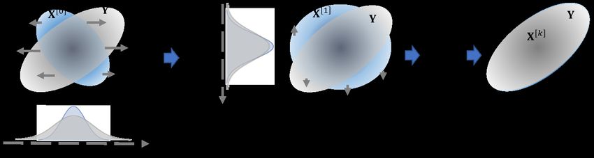
2                                                    Jingyi Zhang, Wenxuan Zhong, and Ping Ma

an operator runs n warehouses and m factories. Each warehouse contains a certain
amount of valuable raw material, i.e., the resources, that is needed by the factories
to run properly. Furthermore, each factory has a certain demand for raw material.
Suppose the total amount of the resources in the warehouse equals the total demand
for the raw material in the factories. The operator aims to move all the resources
from warehouses to factories, such that all the demands for the factories could be
successfully met, and the total transport cost is as small as possible.

Fig. 1 Illustration for the resource allocation problem. The resources in warehouses are marked in
blue, and the demand for each factory is marked in red.

    The resource allocation problem is a typical OT problem in practice. To put these
problems in mathematical language, one can regard the resources as a whole and
the demands as a whole as two probability distributions. For example, the resources
from warehouses in Fig. 1 can be regarded as a non-uniform discrete distribution
supported on three discrete points, and each of the points represents the geographical
location of a particular warehouse. OT methods aim to find a transport map (or
plan), between these two probability distributions with the minimum transport cost.
Formal definitions for the transport map, the transport plan, and the transport cost
will be given in Section 2.
    Nowadays, many modern statistical and machine learning problems can be recast
as finding the optimal transport map (or plan) between two probability distributions.
For example, domain adaptation [72, 17, 30], aims to learn a well-trained model
from a source data distribution and transfer this model to adopt a target data distri-
bution. Another example is deep generative models [40, 66, 5, 14] target at mapping
a fixed distribution, e.g., the standard Gaussian or uniform distribution, to the un-
derlying population distribution of the genuine sample. During recent decades, OT
methods have been reinvigorated in a remarkable proliferation of modern data sci-
ence applications, including machine learning [3, 17, 76, 5, 12, 29, 66], statistics
[19, 13, 74], and computer vision [26, 79, 89, 76].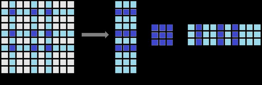
Title Suppressed Due to Excessive Length                                           3

    Although OT finds a large number of applications in practice, the computation
of OT meets challenges in the big data era. Traditional methods estimate the op-
timal transport map (OTM) by solving differential equations [10, 6] or by solving
a problem of linear programming [82, 75]. Consider two p-dimensional samples
with n observations within each sample. The calculation of the OTM between these
two samples using these traditional methods requiring O(n3 log(n)) computational
time [76, 85]. Such a sizable computational cost hinders the broad applicability of
optimal transport methods.
    To alleviate the computational burden for OT, there has been a large number of
work dedicated to developing efficient computational tools in the recent decade.
One class of methods, starting from [18], considers solving a regularized OT prob-
lem instead of the original one. By utilizing the Sinkhorn algorithm (detailed in
Section 3), the computational cost for solving such a regularized problem can be
reduced to O(n2 log(n)), which is a significant reduction from O(n3 log(n)). Based
on this idea, various computational tools are developed to solve the regularized OT
problem as quickly as possible [2, 76]. By combining the Sinkhorn algorithm and
the idea of low-rank matrix approximation, recently, [1] proposed an efficient algo-
rithm with a computational cost that is approximately proportional to n. Although
not covered in this paper, regularization-based optimal transport methods even ap-
pear to have better theoretical properties than the unregularized counterparts; see
[36, 69, 81] for details.
    Another class of methods aims to estimate the OTM efficiently using random or
deterministic projections. These so-called projection-based methods tackle the prob-
lem of estimating a p-dimensional OTM by breaking down the problem into a series
of subproblems, each of which finds a one-dimensional OTM using projected sam-
ples [77, 78, 8, 80]. The subproblems can be easily solved since the one-dimensional
OTM is equivalent to sorting, under some mild conditions. The projection-based
methods reduce the computational cost for calculating OTMs from O(n3 log(n)) to
O(Kn log(n)), where K is the number of iterations until convergence.
    With the help of these computational tools, OT methods have been widely applied
to various biomedical research. Take single-cell RNA sequencing data as an exam-
ple, OT methods can be used to study developmental time courses to infer ancestor-
descendant fates for cells and help researchers to better understand the molecular
programs that guide differentiation during development. For another example, OT
methods can be used as data augmentation tools for increasing the number of obser-
vations; and thus to improve the accuracy and the stability of various downstream
analyses.
    The rest of the paper is organized as follows. We start in Section 2 by introduc-
ing the essential background of the OT problem. In Section 3, we present the details
of regularization-based OT methods and their extensions. Section 4 is devoted to
projection-based OT methods, including both random projection methods and de-
terministic projection methods. In Section 5, we show several applications of OT
methods on real-world problems in biomedical research.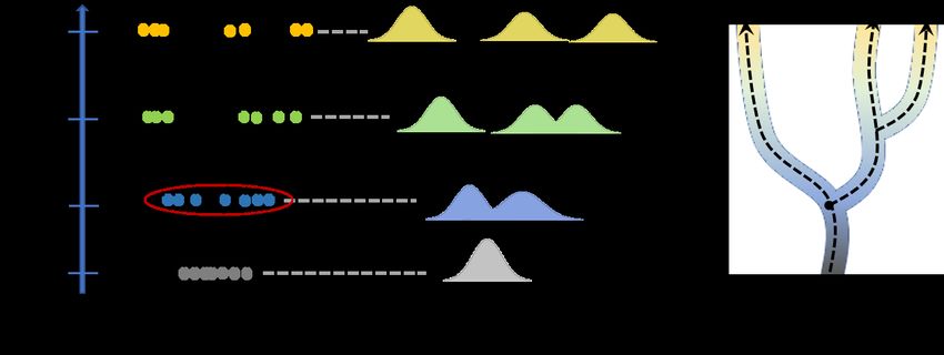
4                                                   Jingyi Zhang, Wenxuan Zhong, and Ping Ma

2 Background of the Optimal Transport Problem

In the aforementioned resource allocation problem, the goal is to transport the re-
sources in the warehouse to the factories with the least cost, say the total fuel con-
sumption of trucks. Here, the resources in the warehouse and the demand in the
factories can be regarded as discrete distributions. We now introduce the following
example that extend the discrete setting to the continuous setting. Suppose there is a
worker who has to move a large pile of sand using a shovel in his hand. The goal of
the worker is to erect with all that sand a target pile with a prescribed shape, say a
sandcastle. Naturally, the worker wishes to minimize the total “effort”, which intu-
itively, in the sense of physical, can be regarded as the “work”, the product of force
and displacement. A French mathematician Gaspard Monge (1746–1818) once con-
sidered such a problem and formulated it into a general Mathematical problem, i.e.,
the optimal transport problem [91, 76]: among all the possible transport maps φ
between two probability measures µ and ν, how to find the one with the minimum
transport cost? Mathematically, the optimal transport problem can be formulated as
follows. Let P(R p ) be the set of Borel probability measures in R p , and let
                                             Z
                   P2 (R ) = µ ∈ P(R ) ||x|| dµ(x) < ∞ .
                          p                 p        2

For µ, ν ∈ P2 (R p ), let Φ be the set of all the so-called measure-preserving maps
φ : R p → R p , such that φ# (µ) = ν and φ#−1 (ν) = µ. Here, # represents the push-
forward operator, such that for any measurable Ω ⊂ R p , φ# (µ)(Ω ) = µ(φ −1 (Ω )).
Among all the maps in Φ, the optimal transport map defined under a cost function
c(·, ·) is
                                         Z
                        φ † := arg inf           c(x, φ (x))dµ(x).                      (1)
                                φ ∈Φ        Rp

One popular choice for the cost function is c(x, y) = kx − yk2 , with which Equa-
tion (1) becomes
                                        Z
                       φ † := arg inf         kx − φ (x)k2 dµ(x).                       (2)
                               φ ∈Φ      Rp

   Equation (2) is called the Monge formulation, and its solution φ † is called the
optimal transport map (OTM), or the Monge map. The well-known Brenier’s The-
orem [9] stated that, when the cost function c(x, y) = kx − yk2 , if at least one of
µ and ν has a density with respect to the Lebesgue measure, then the OTM φ † in
Equation (2) exists and is unique. In other words, the OTM φ † may not exists, i.e.,
the solution of Equation (2) may not be a map, when the conditions of Brenier’s
Theorem is not met. To overcome such a limitation, Kantorovich [43] considered
the following set of “couplings”,
Title Suppressed Due to Excessive Length 5
M (µ, ν) = {π ∈ P(R p × R p ) s.t. ∀ Borel set A, B ⊂ R p ,
π(A × R p ) = µ(A), π(R p × B) = ν(B)}. (3)
Intuitively, a coupling π ∈ M (µ, ν) is a joint distribution of µ and ν, such that two
particular marginal distributions of π are equal to µ and ν, respectively. Instead of
finding the OTM, Kantorovich formulated the optimal transport problem as finding
the optimal coupling,
Z
∗
π := arg inf kx − yk2 dπ(x, y). (4)
π∈M (µ,ν)
Equation (4) is called the Kantorovich formulation (with L2 cost) and its solution π ∗
is called the optimal transport plan (OTP). The key difference between the Monge
formulation and the Kantorovich formulation is that the latter does not require the
solution to be a one-to-one map, as illustrated in Fig. 2.
The Kantorovich formulation is more realistic in practice, compared with the
Monge formulation. Take the resource allocation problem as an example, as de-
scribed in Section 1. It is unreasonable to assume that there always exists a one-to-
one map between warehouses and factories, which can meet all the demands for the
factories. The optimal solution of such resource allocation problems thus is usually
an OTP instead of an OTM. Note that, although the Kantorovich formulation is more
flexible than the Monge formulation, it can be shown that when the OTM exists, the
OTP is equivalent to the OTM.
Close related to the optimal transport problem is the so-called Wasserstein dis-
tance. Intuitively, if we think the optimal transport problem (either in the Monge
formulation or the Kantorovich formulation) as an optimization problem, then the
Wasserstein distance is simply the optimal objective value of such an optimization
problem, with certain power transform. Suppose the OTM φ † exists, the Wasserstein
distance of order k is defined as
Z 1/k
† k
Wk (µ, ν) := kX − φ (X)k dµ . (5)
Rp
Let {xi }ni=1 and {yi }ni=1 be two samples generated from µ and ν, respectively. One
thus can estimate φ † using these two samples, and we let φb† to denote the corre-
Fig. 2 Comparison between
optimal transport map (OTM)
and optimal transport plan
(OTP). Left: an illustration of
OTM, which is a one-to-one
map. Right: an illustration of
OPT, which may not neces-
sarily to be a map.6 Jingyi Zhang, Wenxuan Zhong, and Ping Ma
sponding estimator. The Wasserstein distance Wk (µ, ν) thus can be estimated by
!1/k
1 n
bk (µ, ν) :=
W ∑ kxi − φb† (xi )kk
n i=1
.
The Wasserstein distance respecting to the Kantorovich formulation can be defined
analogously. We refer to [97, 20, 74] and the reference therein for theoretical proper-
ties of Wasserstein distances. Without further notification, we focus on the L2 norm
throughout this paper, i.e., k = 2 in Equation (5), and we abbreviate W2 (µ, ν) by
W (µ, ν).
3 Regularization-based Optimal Transport Methods
In this section, we introduce a family of numerical schemes to approximate solutions
to the Kantorovich formulation (4). Such numerical schemes add a regularization
penalty to the original optimal transport problem, and one can then solve the regular-
ized problem instead. Such a regularization-based approach has long been studied in
nonparametric regression literature to balances the trade-off between the goodness-
of-fit and the model and the roughness of a nonlinear function [41, 57, 100, 68].
Cuturi first introduced the regularization approach in OT problems [18] and
showed that the regularized problem could be solved using a simple alternate min-
imization scheme, requiring O(n2 log(n)p) computational time. Moreover, it can
be shown that the solution to the regularized OT problem can well-approximate
the solution to its unregularized counterpart. We call such numerical schemes the
regularization-based optimal transport methods. We now present the details and
some extensions of these methods as follows.
3.1 Computational Cost for OT Problems
We first introduce how to calculate the empirical Wasserstein distance by solving a
linear system. Let p and q be two probability distributions supported on a discrete
set {xi }ni=1 , where xi ∈ Ω for i = 1, . . . , n, and Ω ⊂ R p is bounded. We identify p
and q as the vectors located on the simplex
( )
n
∆n := v ∈ Rn : ∑ vi = 1, and vi ≥ 0, i = 1, . . . , n. ,
i=1
whose entries denote the weight of each distribution assigned to the points of
{xi }ni=1 . Let C ∈ Rn×n be the pair-wise distance matrix, where Ci j = kxi − x j k2 ,
and 1n be the all-ones vector with n elements. Recall the definition of coupling in
Equation (3), and analogously, we denote by M (p, q) the set of coupling matricesTitle Suppressed Due to Excessive Length 7
between p and q, i.e.,
M (p, q) = P ∈ Rn×n : P1n = p, P| 1n = q .
For brevity, this paper focuses on square matrices C and P, since extensions to
rectangular cases are straightforward.
Let h·, ·i denote the summation of the element-wise multiplication, such that,
for any two matrix A, B ∈ Rn×n , hA, Bi = ∑ni=1 ∑nj=1 Ai j Bi j . According to the Kan-
torovich formulation in Equation (4), the Wasserstein distance between p and q, i.e.,
W (p, q) thus can be calculated through solving the following optimization problem
min hP, Ci , (6)
P∈M (p,q)
which is a linear program with O(n) linear constraints. The coupling matrix P is
called the optimal coupling matrix, when the optimization problem (6) achieves the
minimum value, i.e., the optimal coupling matrix is the minimizer of the optimiza-
tion problem (6). Note that when the OTM exists, the optimal coupling matrix P is a
sparse matrix, such that there is exactly one non-zero element in each row and each
column of P, respectively.
Practical algorithms for solving the problem (6) through linear programming re-
quiring a computational time of the order O(n3 log(n)) for fixed p [76]. Such a siz-
able computational cost hinders the broad applicability of OT methods in practice
for the datasets with large sample size.
3.2 Sinkhorn Distance
To alleviate the computation burden for OT problems, [18] considered a vari-
ant of the minimization problem in Equation (6), which can be solved within
O(n2 log(n)p) computational time using the Sinkhorn scaling algorithm, originally
proposed in [87]. The solution of such a variant is called the Sinkhorn “distance” 1 ,
defined as
Wη (p, q) = min hP, Ci − η −1 H(P), (7)
P∈M (p,q)
where η > 0 is the regularization parameter, and H(P) = ∑ni=1 ∑nj=1 Pi j log(1/Pi j )
is the Shannon entropy of P. We adopt the standard convention that 0 log(1/0) = 0
in the Shannon entropy. We present a fundamental definition as follows [87].
Definition 1. Given p, q ∈ ∆n and K ∈ Rn×n with positive entries, the Sinkhorn
projection ΠM (p,q) (K) of K onto M (p, q) is the unique matrix in M (p, q) of the
form D1 KD2 for positive diagonal matrices D1 , D2 ∈ Rn×n .
1We use quotations here since it is not technically a distance; see Section 3.2 of [18] for details.
The quotes are dropped henceforth.8 Jingyi Zhang, Wenxuan Zhong, and Ping Ma
Let Pη be the minimizer, i.e., the optimal coupling matrix, of the optimiza-
tion problem (7). Throughout the paper, all matrix exponentials and logarithms
will be taken entrywise, i.e., (eA )i j := eAi j and (log A)i j := log Ai j for any matrix
A ∈ Rn×n . [18] built a simple but key connection between the Sinkhorn distance and
the Sinkhorn projection,
Pη = argmin hP, Ci − η −1 H(P)
P∈M (p,q)
= argmin hηC, Pi − η −1 H(P)
P∈M (p,q)
D E
= argmin − log e−ηC , P − η −1 H(P)
P∈M (p,q)
= ΠM (p,q) e−ηC . (8)
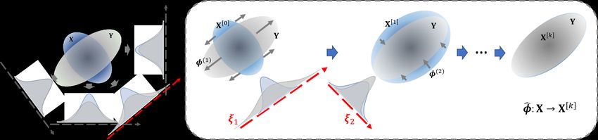
Equation (8) suggests the minimizer of the optimization problem (7) takes the form
D1 (e−ηC )D2 , for some positive diagonal matrices D1 , D2 ∈ Rn×n , as illustrated in
Fig. 3. Moreover, it can be shown that the minimizer in Equation (8) exists and is
unique due to the strict convexity of −H(P) and the compactness of M (p, q).
Fig. 3 The minimizer of the regularized optimal transport problem (7) takes the form D1 (e−ηC )D2 ,
for some unknown diagonal metrics D1 and D2 .
Based on Equation (8), [18] proposed a simple iterative algorithm, which is also
known as the Sinkhorn-Knopp algorithm, to approximate Pη . Let xi , yi , pi , qi be the
i-th element of the vector x, y, p, and q, respectively, for i = 1, . . . , n. For simplicity,
we now use A to denote the matrix e−ηC . Intuitively, the Sinkhorn-Knopp algorithm
works as an alternating projection procedure that renormalizes the rows and columns
of A in turn, so that they match the desired row and column marginals p and q. In
specific, at each step, it prescribes to either modify all the rows of A by multiplying
the i-th row by (pi / ∑nj=1 Ai j ), for i = 1, . . . , n, or to do the analogous operation
on the columns. Here, ∑nj=1 Ai j is simply the i-th row sum of A. Analogously, we
also use ∑ni=1 Ai j to denote the j-th column sum of A. The standard convention that
0/0 = 1 is adopted in the algorithm if it occurs. The algorithm terminates when
the matrix A, after k-th iteration, is sufficiently close to the polytope M (p, q). The
pseudocode for the Sinkhorn-Knopp algorithm is shown in Algorithm 1.Title Suppressed Due to Excessive Length 9
Algorithm 1 S INKHORN (A, M (p, q), ε )
Initialize: k ← 0; A[0] ← A/kAk1 ; x[0] ← 0; y [0] ← 0
repeat
k ← k+1
if k is odd then
[k−1]
xi ← log(pi / ∑nj=1 Ai j ), for i = 1, . . . , n
x[k] ← x[k−1] + x; y [k] ← y [k−1]
else
[k−1]
y j ← log(qi / ∑ni=1 Ai j ), for j = 1, . . . , n
y [k] ← y [k−1] + y; x[k] ← x[k−1]
D1 ← diag(exp(x[k] )); D2 ← diag(exp(y [k] ))
A[k] = D1 AD2
until dist(A[k] , M (p, q)) ≤ ε
Output: Pη = A[k]
One question remaining for Algorithm 1 is how to determine the size of η, which
balances the trade-off between the computation time and the estimation accuracy. In
specific, a small η is associated with a more accurate estimation of the Wasserstein
distance as well as longer computation time [34].
Algorithm 1 requires a computational cost of the order O(n2 log(n)pK), where K
is the number of iterations. It is known that K = O(ε −2 ) in order to let Algorithm 1
to achieve the desired accuracy. Recently, [2] proposed a new greedy coordinate de-
scent variant of the Sinkhorn algorithm with the same theoretical guarantees and a
significantly smaller number of iterations. With the help of Algorithm 1, the regu-
larized optimal transport problem can be solved reliably and efficiently in the cases
when n ≈ 104 [18, 35].
3.3 Sinkhorn Algorithms with the Nyström Method
Although the Sinkhorn-Knopp algorithm has already yielded impressive algorith-
mic benefits, its computational complexity and memory usage are of the order of
n2 , since such an algorithm involves the calculation of the n × n matrix e−ηC . Such
a quadratic computational cost makes the calculation of Sinkhorn distances pro-
hibitively expensive on the datasets with millions of observations.
To alleviate the computation burden, [1] proposed to replace the computation of
the entire matrix e−ηC with its low-rank approximation. Computing such approxi-
mations is a problem that has long been studied in machine learning under different
names, including Nyström method [98, 96], sparse greedy approximations [88], in-
complete Cholesky decomposition [27], and CUR matrix decomposition [64]. These
methods draw great attention in the subsampling literature due to its close rela-
tionship to the algorithmic leveraging approach [59, 67, 100, 60], which has been10 Jingyi Zhang, Wenxuan Zhong, and Ping Ma
widely applied in linear regression models [62, 23, 58], logistic regression [93],
and streaming time series [99]. Among the aforementioned low-rank approxima-
tion methods, the Nyström method is arguably the most extensively used one in
the literature [94, 63]. We now briefly introduce Nyström method, followed by the
fast Sinkhorn algorithm proposed in [1] that utilize Nyström for low-rank matrix
approximation.
Let K ∈ Rn×n be the matrix that we aim to approximate. Let s < n be a positive
integer, S be a n × s column selection matrix 2 , and R = KS ∈ Rn×s be the so-called
sketch matrix of K. In other words, R is a matrix that contains certain columns of
K. Consider the optimization problem
e = argminkS| (K − RXR| )Sk2F ,
X (9)
X∈Rs×s
where k · kF denotes the Frobenius norm. Equation (9) suggests the matrix RXR e |
can be utilized as a low-rank approximation of K, since such a matrix is the closest
one to K among all the semi-positive definite metrics that have rank at most s. Let
(·)+ to denote the Moore-Penrose inverse of a matrix. It is known that the minimizer
of the optimization problem (9) takes the form
e = (S| R)+ (S| KS)(R| S)+ = (S| KS)+ ;
X
see [94] for technical details. Consequently, we have the following low-rank approx-
imation of K,
K ≈ R(S| KS)+ R| ,
and such an approximation is called the Nyström method, as illustrated in Fig. 4. It
is known that the Nyström method is highly efficient, and could reliably be run on
problems of size n ≈ 106 [94].
Fig. 4 Illustration for the Nyström method.
2 A column selection matrix is the one that all the elements of which equals zero except that there
exists one element in each column that equals one.Title Suppressed Due to Excessive Length 11
Algorithm 2 introduces NYS-SINK [1], i.e., the Sinkhorn algorithm imple-
mented with the the Nyström method. The notations are analogous to the ones in
Algorithm 1. Algorithm 2 requires a memory cost of the order O(ns) and a compu-
Algorithm 2 N YS - SINK (A, M (p, q), ε ,s)
Input: A, p, q, s
Step 1: Calculate the Nyström approximation of A (with rank s), denoted by A.
e
Step 2: P = S INKHORN (A, M (p, q), ε )
e η e
Output: P eη
tational cost of the order O(ns2 p). When s
n, these costs are significant reductions
compared with O(n2 ) and O(n2 log(n)p) for Algorithm 1, respectively. [1] reported
that Algorithm 2 could reliably be run on problems of size n ≈ 106 on a single
laptop.
There are two fundamental questions when implementing the Nyström method
in practice: (1) how to decide the size of s; and (2) given s, how to construct the
column selection matrix S. For the latter question, we refer to [37] for an extensive
review of how to construct S through weighted random subsampling. There also
exists recursive strategy [71] for potentially more effective construction of S. For the
former question, various data-driven strategies have been proposed to determine the
size of s that is adaptive to the low-dimensional structure of the data. These strategies
are developed under different model setups, including kernel ridge regression [37,
71, 11], kernel K-means [42, 95], and so on. Recently, [4] further improved the
efficiency through Nesterov’s smoothing technique. Consider the optimal transport
problem that of our interest, [1] assumed the data are lying on a low-dimensional
manifold, and the authors developed a data-driven strategy to determine the effective
dimension of such a manifold.
4 Projection-based Optimal Transport Methods
In the cases when n
p, one can utilize projection-based optimal transport methods
for potential faster calculation as well as smaller memory consumption, compared
with regularization-based optimal transport methods. These projection-based meth-
ods build upon a key fact that the empirical one-dimensional OTM under the L2
norm is equivalent to sorting. Utilizing such a fact, the projection-based OT meth-
ods tackle the problem of estimating a p-dimensional OTM by breaking down the
problem into a series of subproblems, each of which finds a one-dimensional OTM
using projected samples [77, 78, 8, 80]. The projection direction can be selected
either at random or at deterministic, based on different criteria. Generally speaking,
the computational cost for these projection-based methods are approximately pro-
portional to n, and the memory cost of which is at the order of O(np), which is a12 Jingyi Zhang, Wenxuan Zhong, and Ping Ma
significant reduction from O(n2 ) when p
n. We will cover some representatives
of the projection-based OT methods in this section.
4.1 Random Projection OT Method
The random projection method, also called the Radon probability density func-
tion (PDF) transformation method, is first proposed in [77] for transferring the
color between different images. Intuitively, an image can be represented as a three-
dimensional sample in the RGB color space, in which each pixel of the image is
an observation. The goal of color transfer is to find a transport map φ such that the
color of the transformed source image follows the same distribution of the color of
the target image. Although the map φ does not have to be the OTM in this problem,
the random projection method proposed in [77] can be regarded as an estimation
method for OTM.
The random projection method is built upon the fact that two PDFs are identical
if the marginal distributions, respecting all possible one-dimensional projection di-
rections, of these two PDFs, are identical. Since it is impossible to consider all possi-
ble projection directions in practice, the random projection method thus utilizes the
Monte Carlo method and considers a sequence of randomly generated projection
directions. The details of the random projection method are summarized in Algo-
rithm 3. The computational cost for Algorithm 3 is at the order of O(n log(n)pK),
where K is the number of iterations under converge. We illustrate Algorithm 3 in
Fig. 5.
Algorithm 3 Random projection method for OTM
Input: the source matrix X ∈ Rn×p and the target matrix Y ∈ Rn×p
k ← 0, X[0] ← X
repeat
(a) generate a random projection direction ζk ∈ R p
(b) find the one-dimensional OTM φ (k) that matches X[k] ζk to Yζk
(c) X[k+1] ← X[k] + (φ (k) (X[k] ζk ) − X[k] ζk )ζk|
(d) k ← k + 1
until converge
The final estimator is given by φb : X → X[k]
Instead of randomly generating the projection directions using the Monte Carlo
method, one can also generate a sequence of projection directions with “low-
discrepancy”, i.e., the directions that are distributed as disperse as possible on the
unit sphere. The low-discrepancy sequence has been widely applied in the field of
quasi-Monte Carlo and has been extensively employed for numerical integration
[73] and subsampling in big data [68]. We refer to [49, 50, 21, 38] for more in-depthTitle Suppressed Due to Excessive Length 13
Fig. 5 Illustration of Algorithm 3. In the k-th iteration, a random projection direction ζk is gener-
ated, and the one-dimensional OTM is calculated that match the projected sample X[k] ζk to Yζk .
discussions on quasi-Monte Carlo methods. It is reported in [77] that using a low-
discrepancy sequence of projection directions yields a potentially faster convergence
rate.
Close related to the random projection method is the sliced method. The sliced
method modifies the random projection method by considering a large set of ran-
dom directions from Sd−1 in each iteration, where Sd−1 is the d-dimensional unit
sphere. The “mean map” of the one-dimensional OTMs over these random direc-
tions is considered as a component of the final estimate of the desired OTM. Let L be
the number of projection directions considered in each iteration. Consequently, the
computational cost of the sliced method is at the order of O(n log(n)pKL), where K
is the number of iterations until convergence. Although the sliced method is L times
slower than the random projection method, in practice, it is usually observed that
the former yields a more robust estimation of the latter. We refer to [8, 80] for more
implementation details of the sliced method.
4.2 Projection Pursuit OT Method
Despite the random projection method works reasonably well in practice, for mod-
erate or large p, such a method suffers from slow or none convergence due to the
nature of randomly selected projection directions. To address this issue, [66] intro-
duced a novel statistical approach to estimate large-scale OTMs 3 . The proposed
method, named projection pursuit Monge map (PPMM), combines the idea of pro-
jection pursuit [33] and sufficient dimension reduction [51]. The projection pursuit
technique is similar to boosting that search for the next optimal direction based on
the residual of previous ones. In each iteration, PPMM aims to find the “optimal”
projection direction, guided by sufficient dimension reduction techniques, instead of
using a randomly selected one. Utilizing these informative projection directions, it
is reported in [66] that the PPMM method yields a significantly faster convergence
rate than the random projection method. We now introduce some essential back-
3 The code is available at https://github.com/ChengzijunAixiaoli/PPMM.14 Jingyi Zhang, Wenxuan Zhong, and Ping Ma
ground of sufficient dimension reduction techniques, followed by the details of the
PPMM method.
Consider a regression problem with a univariate response T and a p-dimensional
predictor Z. Sufficient dimension reduction techniques aim to reduce the dimension
of Z while preserving its regression relation with T . In other words, such tech-
niques seek a set of linear combinations of Z, say B| Z with some projection matrix
B ∈ R p×q (q < p), such that T depends on Z only through B| Z, i.e.,
⊥ Z|B| Z.
T⊥ (10)
Let S (B) to denote the column space of B. We call S (B) a sufficient dimen-
sion reduction subspace (s.d.r. subspace) if B satisfy Formulation (10). Moreover,
if the intersection of all possible s.d.r. subspaces is still an s.d.r. subspace, we call
it the central subspace and denote it as ST |Z . Note that the central subspace is the
s.d.r. subspace with the minimum number of dimensions. Some popular sufficient
dimension reduction techniques include sliced inverse regression (SIR) [53], princi-
pal Hessian directions (PHD) [54], sliced average variance estimator (SAVE) [16],
directional regression (DR) [52], among others. Under some regularity conditions,
it can be shown that these methods can induce an s.d.r. subspace that equals the
central subspace.
Consider estimating the OTM between a source sample and a target sample. One
can form a regression problem using these two samples, i.e., add a binary response
variable by labeling them as 0 and 1, respectively. The PPMM method utilizes suf-
ficient dimension reduction techniques to select the most “informative” projection
direction. Here, we call a projection direction ξ the most informative one, if the
projected samples have the most substantial “ discrepancy.” The discrepancy can be
measured by the difference of the kth order moments or central moments. For exam-
ple, the SIR method measures the discrepancy using the difference of means, while
the SAVE method measures the discrepancy using the difference of variances. The
authors in [66] considered the SAVE method and showed that the most informative
projection direction was equivalent to the eigenvector corresponding to the largest
eigenvalue of the projection matrix B, estimated by SAVE. The detailed algorithm
for PPMM is summarized in Algorithm 4 as follows.
The computational cost for Algorithm 4 mainly resides in steps (a) and (b).
Within each iteration, steps (a) and (b) require the computational cost of the or-
der O(np2 ) and O(n log(n), respectively. Consequently, the overall computational
cost for Algorithm 4 is at the order of O(Knp2 + Kn log(n)), where K is the number
of iterations. Although not theoretical guaranteed, it is reported in [66] that K is ap-
proximately proportional to p in practice, in which case the computational cost for
PPMM becomes O(np3 + n log(n)p). Compared with the computational cost for the
Sinkhorn algorithm, i.e., O(n2 log(n)p), PPMM has a lower order of the computa-
tional cost when p
n. We illustrate Algorithm 4 in Fig. 6. Although not covered
in this section, the PPMM method can be easily extended to calculate the OTP, with
minor modifications [66].Title Suppressed Due to Excessive Length 15
Algorithm 4 Projection pursuit Monge map (PPMM)
Input: two matrix X ∈ Rn×p and Y ∈ Rn×p
k ← 0, X[0] ← X
repeat
(a) calculate the most informative projection direction ξk ∈ R p between X[k]
and Y using SAVE
(b) find the one-dimensional OTM φ (k) that matches X[k] ξk to Yξk
(c) X[k+1] ← X[k] + (φ (k) (X[k] ξk ) − X[k] ξk )ξk|
(d) k ← k + 1
until converge
The final estimator is given by φb : X → X[k]
Fig. 6 Illustration of Algorithm 4. The left panel shows that in the k-th iteration, the most informa-
tive projection direction ξk is calculated by SAVE. The right panel shows that the one-dimensional
OTM is calculated to match the projected sample X[k] ξk to Yξk .
5 Applications in Biomedical Research
In this section, we present some cutting-edge applications of optimal transport meth-
ods in biomedical research. We first present how optimal transport methods can be
utilized to identify developmental trajectories of single cells [84]. We then review
a novel method for augmenting the single-cell RNA-seq data [65]. The method uti-
lizes the technique of generative adversarial networks (GAN), which is closely re-
lated to optimal transport methods, as we will discuss later.
5.1 Identify Development Trajectories in Reprogramming
The rapid development of single-cell RNA sequencing (scRNA-seq) technologies
has enabled researchers to identify cell types in a population. These technologies
help researchers to answer some fundamental questions in biology, including how
individual cells differentiate to form tissues, how tissues function in a coordinated
and flexible fashion, and which gene regulatory mechanisms support these processes
[90].
Although sc-RNA-seq technologies have been opening up new ways to tackle
the aforementioned questions, other questions remain. Since these technologies re-16 Jingyi Zhang, Wenxuan Zhong, and Ping Ma quire to destroy cells in the course of sequencing their gene expression profiles, re- searchers cannot follow the expression of the same cell across time. Without further analysis, researchers thus are not able to answer the questions like what was the ori- gin of certain cells at earlier stages and their possible fates at later stages; what and how regulatory programs control the dynamics of cells? To answer these questions, one natural solution is to develop computational tools to connect the cells within different time points into a continuous cell trajectory. In other words, although dif- ferent cells are recorded in each time point, for each cell, the goal is to identify the ones that are analogous to its origins and its fates in earlier stages and late stages, respectively. A large number of methods have been developed to achieve this goal; see [44, 83, 25, 28] and the reference therein. A novel approach was proposed in [90] to reconstruct cell trajectories. They model the differentiating population of cells as a stochastic process on a high- dimensional expression space. Recall that different cells are recorded independently at different time points. Consequently, the unknown fact to the researchers is the joint distribution of expression of the unobserved cells between different pairs of time points. To infer how the differentiation process evolves over time, the authors assume the expression of each cell changes within a relatively small range over short periods. Based on such an assumption, one thus can infer the differentiation process though optimal transport methods, which naturally gives the transport map between two distributions, respecting to two time points, with the minimum transport cost. Figure 7 illustrates an idea to search for the “cell trajectories”. For gene expres- sion Xt of any set of cells at time t, it can be transported to a later time point t + 1 according to OTP from the distribution over Xt to the distribution over the cells at time t + 1. Analogously, Xt can be transported from a former time point t − 1 by back-winding the OPT from the distribution over Xt to the distribution over the cells at time t − 1 (The left and middle panels in Fig. 7). The trajectory combines the transportation between any two neiboring time points (The right panel in Fig. 7). Thus, OTP helps to infer the differentiation process of cells the at any time along the trajectory. Fig. 7 Illustration for cell trajectories along time. Left: cells at each time point. Middle: OPT between distributions over cells at each time point. Right: cell trajectories based on OPT.
Title Suppressed Due to Excessive Length                                            17

   The authors in [90] used optimal transport methods to calculate the differenti-
ation process between consecutive time points and then compose all the transport
maps together to obtain the cell trajectories over long time-intervals. The authors
also considered unbalanced transport [15] for modeling cellular proliferation, i.e.,
cell growth and death. Analyzing around 315,000 cell profiles sampled densely
across 18 days, the authors found reprogramming unleashes a much wider range
of developmental programs and subprograms than previously characterized.

5.2 Data Augmentation for Biomedical Data

Recent advances in scRNA-seq technologies have enabled researchers to measure
the expression of thousands of genes at the same time and to scrutinize the complex
interactions in biological systems. Despite wide applications, such technologies may
fail to quantify all the complexity in biological systems in the cases when the num-
ber of observations is relatively small, due to economic or ethical considerations or
simply because the sample size of available patients is low [70]. The problem of a
small sample size results in biased results since a small sample may not be a decent
representative of the population.
    Not only arising from biomedical research, such a problem also arises from the
research in various fields, including computer vision and deep learning, which re-
quire considerable quantity and diversity of data during the training process [46, 39].
In these fields, data augmentation is a widely-applied strategy to alleviate the prob-
lem of small sample sizes, without actually collecting new data. In computer vision,
some elementary algorithms for data augmentation include cropping, rotating, and
flipping; see [86] for a survey. These algorithms, however, may not be suitable for
augmenting data in biomedical research.
    Compared with these elementary algorithms, a more sophisticated approach for
data augmentation is to use generative models, including generative adversarial nets
(GAN) [40], the “decoder” network in variational autoencoders [45], among others.
Generative models aim to generate “fake” samples that are indistinguishable from
the genuine ones. The fake samples then can be used, alongside the genuine ones, in
down-stream analysis to artificially increase sample sizes. Generative models have
been widely used for generating realistic images [22, 56], songs [7, 24], and videos
[55, 92]. Many variants of the GAN method have been proposed recently, and of
particular interest is the Wasserstein GAN [5], which utilizes the Wasserstein dis-
tance instead of the Jensen–Shannon divergence in the standard GAN for measur-
ing the discrepancy between two samples. The authors showed that the Wasserstein
GAN yields a more stable training process compared with the standard GAN, since
Wasserstein distance appears to be a more powerful metric than the Jensen–Shannon
divergence in GAN.
    Nowadays, GAN has been widely used for data augmentation in various biomedi-
cal research [32, 31, 61]. Recently, [65] proposed a novel data augmentation method
for scRNA-seq data. The proposed method, called single-cell GAN, is developed
18 Jingyi Zhang, Wenxuan Zhong, and Ping Ma
based on Wasserstein GAN. The authors showed the proposed method improves
downstream analyses such as the detection of marker genes, the robustness and re-
liability of classifiers, and the assessment of novel analysis algorithms, resulting in
the potential reduction of the number of animal experiments and costs.
Note that generative models are closely related to optimal transport methods. In-
tuitively, a generative model is equivalent to finding a transport map from random
noises with a simple distribution, e.g., Gaussian distribution or uniform distribution,
to the underlying population distribution of the genuine sample. Recent studies sug-
gest optimal transport methods outperform the Wasserstein GAN for approximating
probability measures in some special cases [48, 47]. Consequently, researchers may
consider using optimal transport methods instead of GAN models for data augmen-
tation in biomedical research for potentially better performance.
Acknowledgment
The authors would like to acknowledge the support from the U.S. National Science
Foundation under grants DMS-1903226, DMS-1925066, the U.S. National Institute
of Health under grant R01GM122080.
References
1. J. Altschuler, F. Bach, A. Rudi, and J. Niles-Weed. Massively scalable sinkhorn distances via
the nyström method. In Advances in Neural Information Processing Systems, pages 4429–
4439, 2019.
2. J. Altschuler, J. Weed, and P. Rigollet. Near-linear time approximation algorithms for optimal
transport via sinkhorn iteration. In Advances in Neural Information Processing Systems,
pages 1964–1974, 2017.
3. D. Alvarez-Melis, T. Jaakkola, and S. Jegelka. Structured optimal transport. In International
Conference on Artificial Intelligence and Statistics, pages 1771–1780, 2018.
4. D. An, N. Lei, and X. Gu. Efficient optimal transport algorithm by accelerated gradient
descent. arXiv preprint arXiv:2104.05802, 2021.
5. M. Arjovsky, S. Chintala, and L. Bottou. Wasserstein generative adversarial networks. In
International Conference on Machine Learning, pages 214–223, 2017.
6. J.-D. Benamou, Y. Brenier, and K. Guittet. The monge–kantorovitch mass transfer and its
computational fluid mechanics formulation. International Journal for Numerical methods in
fluids, 40(1-2):21–30, 2002.
7. M. Blaauw and J. Bonada. Modeling and transforming speech using variational autoen-
coders. In Interspeech, pages 1770–1774, 2016.
8. N. Bonneel, J. Rabin, G. Peyré, and H. Pfister. Sliced and radon wasserstein barycenters of
measures. Journal of Mathematical Imaging and Vision, 51(1):22–45, 2015.
9. Y. Brenier. Polar factorization and monotone rearrangement of vector-valued functions.
Communications on pure and applied mathematics, 44(4):375–417, 1991.
10. Y. Brenier. A homogenized model for vortex sheets. Archive for Rational Mechanics and
Analysis, 138(4):319–353, 1997.
11. D. Calandriello, A. Lazaric, and M. Valko. Analysis of nyström method with sequential ridge
leverage score sampling. 2020.Title Suppressed Due to Excessive Length 19
12. G. Canas and L. Rosasco. Learning probability measures with respect to optimal transport
metrics. In Advances in Neural Information Processing Systems, pages 2492–2500, 2012.
13. E. Cazelles, V. Seguy, J. Bigot, M. Cuturi, and N. Papadakis. Geodesic pca versus log-pca
of histograms in the wasserstein space. SIAM Journal on Scientific Computing, 40(2):B429–
B456, 2018.
14. Y. Chen, T. T. Georgiou, and A. Tannenbaum. Optimal transport for gaussian mixture models.
IEEE Access, 7:6269–6278, 2018.
15. L. Chizat, G. Peyré, B. Schmitzer, and F.-X. Vialard. Scaling algorithms for unbalanced
optimal transport problems. Mathematics of Computation, 87(314):2563–2609, 2018.
16. R. D. Cook and S. Weisberg. Sliced inverse regression for dimension reduction: Comment.
Journal of the American Statistical Association, 86(414):328–332, 1991.
17. N. Courty, R. Flamary, D. Tuia, and A. Rakotomamonjy. Optimal transport for domain
adaptation. IEEE transactions on pattern analysis and machine intelligence, 39(9):1853–
1865, 2016.
18. M. Cuturi. Sinkhorn distances: Lightspeed computation of optimal transport. In Advances in
neural information processing systems, pages 2292–2300, 2013.
19. E. Del Barrio, P. Gordaliza, H. Lescornel, and J.-M. Loubes. Central limit theorem and
bootstrap procedure for wasserstein’s variations with an application to structural relationships
between distributions. Journal of Multivariate Analysis, 169:341–362, 2019.
20. E. Del Barrio and J.-M. Loubes. Central limit theorems for empirical transportation cost in
general dimension. The Annals of Probability, 47(2):926–951, 03 2019.
21. J. Dick, F. Y. Kuo, and I. H. Sloan. High-dimensional integration: the quasi-monte carlo way.
Acta Numerica, 22:133–288, 2013.
22. A. Dosovitskiy and T. Brox. Generating images with perceptual similarity metrics based on
deep networks. In Advances in neural information processing systems, pages 658–666, 2016.
23. P. Drineas, M. Magdon-Ismail, M. W. Mahoney, and D. P. Woodruff. Fast approxima-
tion of matrix coherence and statistical leverage. Journal of Machine Learning Research,
13(Dec):3475–3506, 2012.
24. J. Engel, C. Resnick, A. Roberts, S. Dieleman, M. Norouzi, D. Eck, and K. Simonyan. Neural
audio synthesis of musical notes with wavenet autoencoders. In Proceedings of the 34th
International Conference on Machine Learning-Volume 70, pages 1068–1077. JMLR. org,
2017.
25. J. A. Farrell, Y. Wang, S. J. Riesenfeld, K. Shekhar, A. Regev, and A. F. Schier. Single-
cell reconstruction of developmental trajectories during zebrafish embryogenesis. Science,
360(6392):eaar3131, 2018.
26. S. Ferradans, N. Papadakis, G. Peyré, and J.-F. Aujol. Regularized discrete optimal transport.
SIAM Journal on Imaging Sciences, 7(3):1853–1882, 2014.
27. S. Fine and K. Scheinberg. Efficient svm training using low-rank kernel representations.
Journal of Machine Learning Research, 2(Dec):243–264, 2001.
28. D. S. Fischer, A. K. Fiedler, E. M. Kernfeld, R. M. Genga, A. Bastidas-Ponce, M. Bakhti,
H. Lickert, J. Hasenauer, R. Maehr, and F. J. Theis. Inferring population dynamics from
single-cell rna-sequencing time series data. Nature biotechnology, 37(4):461–468, 2019.
29. R. Flamary, M. Cuturi, N. Courty, and A. Rakotomamonjy. Wasserstein discriminant analy-
sis. Machine Learning, 107(12):1923–1945, 2018.
30. R. Flamary, K. Lounici, and A. Ferrari. Concentration bounds for linear monge mapping
estimation and optimal transport domain adaptation. arXiv preprint arXiv:1905.10155, 2019.
31. M. Frid-Adar, I. Diamant, E. Klang, M. Amitai, J. Goldberger, and H. Greenspan. Gan-
based synthetic medical image augmentation for increased cnn performance in liver lesion
classification. Neurocomputing, 321:321–331, 2018.
32. M. Frid-Adar, E. Klang, M. Amitai, J. Goldberger, and H. Greenspan. Synthetic data aug-
mentation using gan for improved liver lesion classification. In 2018 IEEE 15th international
symposium on biomedical imaging (ISBI 2018), pages 289–293. IEEE, 2018.
33. J. H. Friedman and W. Stuetzle. Projection pursuit regression. Journal of the American
statistical Association, 76(376):817–823, 1981.20 Jingyi Zhang, Wenxuan Zhong, and Ping Ma
34. A. Genevay, L. Chizat, F. Bach, M. Cuturi, and G. Peyré. Sample complexity of sinkhorn
divergences. In The 22nd International Conference on Artificial Intelligence and Statistics,
pages 1574–1583, 2019.
35. A. Genevay, M. Cuturi, G. Peyré, and F. Bach. Stochastic optimization for large-scale optimal
transport. In Advances in neural information processing systems, pages 3440–3448, 2016.
36. A. Genevay, G. Peyré, and M. Cuturi. Learning generative models with sinkhorn divergences.
arXiv preprint arXiv:1706.00292, 2017.
37. A. Gittens and M. W. Mahoney. Revisiting the nyström method for improved large-scale
machine learning. The Journal of Machine Learning Research, 17(1):3977–4041, 2016.
38. P. Glasserman. Monte Carlo methods in financial engineering, volume 53. Springer Science
& Business Media, 2013.
39. I. Goodfellow, Y. Bengio, and A. Courville. Deep learning. MIT press, 2016.
40. I. Goodfellow, J. Pouget-Abadie, M. Mirza, B. Xu, D. Warde-Farley, S. Ozair, A. Courville,
and Y. Bengio. Generative adversarial nets. In Advances in neural information processing
systems, pages 2672–2680, 2014.
41. C. Gu. Smoothing spline ANOVA models. Springer Science & Business Media, 2013.
42. L. He and H. Zhang. Kernel k-means sampling for nyström approximation. IEEE Transac-
tions on Image Processing, 27(5):2108–2120, 2018.
43. L. Kantorovich. On translation of mass (in russian), c r. In Doklady. Acad. Sci. USSR,
volume 37, pages 199–201, 1942.
44. L. Kester and A. van Oudenaarden. Single-cell transcriptomics meets lineage tracing. Cell
Stem Cell, 23(2):166–179, 2018.
45. D. P. Kingma and M. Welling. Auto-encoding variational bayes. arXiv preprint
arXiv:1312.6114, 2013.
46. Y. LeCun, Y. Bengio, and G. Hinton. Deep learning. nature, 521(7553):436–444, 2015.
47. N. Lei, D. An, Y. Guo, K. Su, S. Liu, Z. Luo, S.-T. Yau, and X. Gu. A geometric understand-
ing of deep learning. Engineering, 2020.
48. N. Lei, K. Su, L. Cui, S.-T. Yau, and X. D. Gu. A geometric view of optimal transportation
and generative model. Computer Aided Geometric Design, 68:1–21, 2019.
49. C. Lemieux. Monte Carlo and quasi-Monte Carlo sampling. Springer, New York, 2009.
50. G. Leobacher and F. Pillichshammer. Introduction to quasi-Monte Carlo integration and
applications. Springer, 2014.
51. B. Li. Sufficient dimension reduction: Methods and applications with R. Chapman and
Hall/CRC, 2018.
52. B. Li and S. Wang. On directional regression for dimension reduction. Journal of the Amer-
ican Statistical Association, 102(479):997–1008, 2007.
53. K.-C. Li. Sliced inverse regression for dimension reduction. Journal of the American Statis-
tical Association, 86(414):316–327, 1991.
54. K.-C. Li. On principal hessian directions for data visualization and dimension reduction:
Another application of stein’s lemma. Journal of the American Statistical Association,
87(420):1025–1039, 1992.
55. X. Liang, L. Lee, W. Dai, and E. P. Xing. Dual motion gan for future-flow embedded video
prediction. In Proceedings of the IEEE International Conference on Computer Vision, pages
1744–1752, 2017.
56. Y. Liu, Z. Qin, Z. Luo, and H. Wang. Auto-painter: Cartoon image generation from sketch by
using conditional generative adversarial networks. arXiv preprint arXiv:1705.01908, 2017.
57. P. Ma, J. Z. Huang, and N. Zhang. Efficient computation of smoothing splines via adaptive
basis sampling. Biometrika, 102(3):631–645, 2015.
58. P. Ma, M. W. Mahoney, and B. Yu. A statistical perspective on algorithmic leveraging.
Journal of Machine Learning Research, 16(1):861–911, 2015.
59. P. Ma and X. Sun. Leveraging for big data regression. Wiley Interdisciplinary Reviews:
Computational Statistics, 7(1):70–76, 2015.
60. P. Ma, X. Zhang, X. Xing, J. Ma, and M. W. Mahoney. Asymptotic analysis of sampling
estimators for randomized numerical linear algebra algorithms. The 23nd International Con-
ference on Artificial Intelligence and Statistics. 2020, 2020.Title Suppressed Due to Excessive Length 21
61. A. Madani, M. Moradi, A. Karargyris, and T. Syeda-Mahmood. Chest x-ray generation
and data augmentation for cardiovascular abnormality classification. In Medical Imaging
2018: Image Processing, volume 10574, page 105741M. International Society for Optics
and Photonics, 2018.
62. M. W. Mahoney. Randomized algorithms for matrices and data. Foundations and Trends®
in Machine Learning, 3(2):123–224, 2011.
63. M. W. Mahoney. Lecture notes on randomized linear algebra. arXiv preprint
arXiv:1608.04481, 2016.
64. M. W. Mahoney and P. Drineas. Cur matrix decompositions for improved data analysis.
Proceedings of the National Academy of Sciences, 106(3):697–702, 2009.
65. M. Marouf, P. Machart, V. Bansal, C. Kilian, D. S. Magruder, C. F. Krebs, and S. Bonn.
Realistic in silico generation and augmentation of single-cell rna-seq data using generative
adversarial networks. Nature Communications, 11(1):1–12, 2020.
66. C. Meng, Y. Ke, J. Zhang, M. Zhang, W. Zhong, and P. Ma. Large-scale optimal transport
map estimation using projection pursuit. In Advances in Neural Information Processing
Systems, pages 8116–8127, 2019.
67. C. Meng, Y. Wang, X. Zhang, A. Mandal, P. Ma, and W. Zhong. Effective statistical methods
for big data analytics. Handbook of Research on Applied Cybernetics and Systems Science,
page 280, 2017.
68. C. Meng, X. Zhang, J. Zhang, W. Zhong, and P. Ma. More efficient approximation of smooth-
ing splines via space-filling basis selection. Biometrika, 2020.
69. G. Montavon, K.-R. Müller, and M. Cuturi. Wasserstein training of restricted boltzmann
machines. In Advances in Neural Information Processing Systems, pages 3718–3726, 2016.
70. M. R. Munafò, B. A. Nosek, D. V. Bishop, K. S. Button, C. D. Chambers, N. P. Du Sert,
U. Simonsohn, E.-J. Wagenmakers, J. J. Ware, and J. P. Ioannidis. A manifesto for repro-
ducible science. Nature human behaviour, 1(1):1–9, 2017.
71. C. Musco and C. Musco. Recursive sampling for the nystrom method. In Advances in Neural
Information Processing Systems, pages 3833–3845, 2017.
72. B. Muzellec and M. Cuturi. Subspace detours: Building transport plans that are optimal on
subspace projections. In Advances in Neural Information Processing Systems, pages 6914–
6925, 2019.
73. A. B. Owen. Quasi-monte carlo sampling. Monte Carlo Ray Tracing: Siggraph, 1:69–88,
2003.
74. V. M. Panaretos and Y. Zemel. Statistical aspects of wasserstein distances. Annual review of
statistics and its application, 6:405–431, 2019.
75. O. Pele and M. Werman. Fast and robust earth mover’s distances. In 2009 IEEE 12th
International Conference on Computer Vision, pages 460–467. IEEE, 2009.
76. G. Peyré, M. Cuturi, et al. Computational optimal transport. Foundations and Trends® in
Machine Learning, 11(5-6):355–607, 2019.
77. F. Pitie, A. C. Kokaram, and R. Dahyot. N-dimensional probability density function transfer
and its application to color transfer. In Computer Vision, 2005. ICCV 2005. Tenth IEEE
International Conference on, volume 2, pages 1434–1439. IEEE, 2005.
78. F. Pitié, A. C. Kokaram, and R. Dahyot. Automated colour grading using colour distribution
transfer. Computer Vision and Image Understanding, 107(1-2):123–137, 2007.
79. J. Rabin, S. Ferradans, and N. Papadakis. Adaptive color transfer with relaxed optimal trans-
port. In 2014 IEEE International Conference on Image Processing (ICIP), pages 4852–4856.
IEEE, 2014.
80. J. Rabin, G. Peyré, J. Delon, and M. Bernot. Wasserstein barycenter and its application to
texture mixing. In International Conference on Scale Space and Variational Methods in
Computer Vision, pages 435–446. Springer, 2011.
81. P. Rigollet and J. Weed. Entropic optimal transport is maximum-likelihood deconvolution.
Comptes Rendus Mathematique, 356(11-12):1228–1235, 2018.
82. Y. Rubner, L. J. Guibas, and C. Tomasi. The earth mover’s distance, multi-dimensional
scaling, and color-based image retrieval. In Proceedings of the ARPA image understanding
workshop, volume 661, page 668, 1997.You can also read