VORTEXNET: LEARNING COMPLEX DYNAMIC SYS- TEMS WITH PHYSICS-EMBEDDED NETWORKS
←
→
Page content transcription
If your browser does not render page correctly, please read the page content below
Under review as a conference paper at ICLR 2021

VORTEX N ET: L EARNING C OMPLEX DYNAMIC S YS -
TEMS WITH P HYSICS -E MBEDDED N ETWORKS

 Anonymous authors
 Paper under double-blind review

                                             A BSTRACT
         In this paper, we present a novel physics-rooted network structure that dramati-
         cally facilitates the learning of complex dynamic systems. Our method is inspired
         by the Vortex Method in fluid dynamics, whose key idea lies in that, given the
         observed flow field, instead of describing it with a function of space and time,
         one can equivalently understand the observation as being caused by a number of
         Lagrangian particles —– vortices, flowing with the field. Since the number of
         such vortices are much smaller than that of the Eulerian, grid discretization, this
         Lagrangian discretization in essence encodes the system dynamics on a compact
         physics-based latent space. Our method enforces such Lagrangian discretization
         with a Encoder—Dynamics—Decode network structure, and trains it with a novel
         three-stage curriculum learning algorithm. With data generated from the high
         precision Eulerian DNS method, our alorithm takes advantage of the simplify-
         ing power of the Lagrangian method while persisting the physical integrity. This
         method fundamentally differs from the current approaches in the field of physics-
         informed learning, and provides superior results for being more versatile, yielding
         more physical-correctness with less data sample, and faster to compute at high
         precision. Beyond providing a viable way of simulating complex fluid at high-
         precision, our method opens up a brand new horizon for embedding knowledge
         prior via constructing physically-valid latent spaces, which can be applied to fur-
         ther research areas beyond physical simulation.

1   I NTRODUCTION
In the quest of understanding the physical world we inhabit, we are all too often thwarted by systems
too complex, too chaotic, and too obscure to grasp, ones we simply cannot get a full understanding of
using the existing first-principles (33). Among these systems, one of the most long standing and vi-
sually exciting one is the dynamics of complex, unsteady fluid flows characterized by high Reynolds
number. Due to the high number of degrees-of-freedom in the motion space, the complex nonlinear
coupling between particles, and the susceptibility to numerical dissipation, to reproduce the behavior
of such fluids in a physically-accurate manner presents a challenging and often intractable problem
for the traditional Computational Fluid Dynamics community (2).
In the last decade, with the drastic advancement in computational power and data availability, we
are presented with the new hope of approaching these previously elusive systems from a new angle:
a data-driven one powered by machine learning(1; 10; 11; 29; 13). Due to the fact that brute-
force machine learning with conventional toolkits such as deep neural networks typically suffers
from the high dimensionality of input-output spaces, expensive cost of data, the tendency to yield
physically implausible results, and the inability to robustly handle extrapolation, recent research
interests have been focused on embedding physical priors in learning algorithms so that the networks
approach the data not as wide-eyed infants but as physicists familiar with the fundamental rules of
how our world operates. In the realm of learning complex fluid dynamics, various works have
been proposed along this line of thinking, seeking to engrave the structure of partial differential
equations (PDE) into the network architecures (44; 28; 5; 23; 39; 25). Although yielding promising
results, these existing methods are profoundly limited due to the fact that they are trying to use
neural networks to learn Partial Differential Equations, which are supposed to be generic to initial
conditions, relying on certain Solver neural networks conditioned to data, which are contingent
to specific initial conditions. Ideally, to obtain initial-condition invariance, the Partial Differential

                                                   1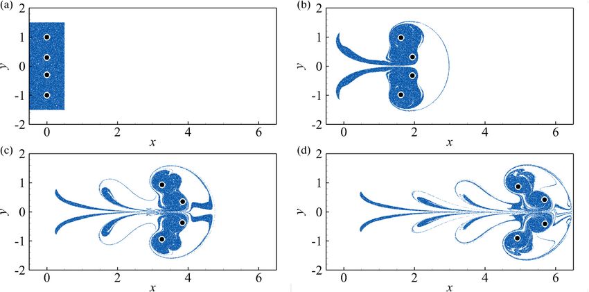
Under review as a conference paper at ICLR 2021

Equation should learn to evolve the flow field without consulting the particular Solver networks, but
due to the high dimensionality and the lack of supervision, such task has not been solved by the
machine learning community to date.
In this work, we propose a novel approach to embed physical prior knowledge to elegantly achieve
invariance to initial conditions, while at the same time being efficient in data usage, easy to im-
plement, fast to compute, adaptable to arbitrary high precisiona and suitable for handling complex,
unsteady flows. Our method is inspired by the Vortex Method in fluid dynamics, who discretizes the
Navier-Stokes equations with a set of Lagrangian particles —– vortices, based on the Helmholtz’s
theorems which states that the behavior of the fluid can be described by a number of vortex elements
flowing with the fluid (2). In the same spirit, our method learns to describe a complex fluid dynamics
system by first learning to associate a small number of Lagrangian vortex particles to the observa-
tion, and simulate the forward dynamics of these vortices instead. This approach can be viewed as
identifying a compact, physics-base latent space where simulation can be performed on efficiently.
To view it another way, instead of tailoring our networks to solve the governing PDEs, we de-
sign our networks to describe the underlying behavior about our system that such equation are
proven to imply. We show the superiority of our vortex-based approach to the previous approaches
with its ability to generalize to different initial conditions, adapt to arbitrary precision, learn with
small data sizes, and to simulate complex, turbulent flows.
To the best of our knowledge, our work is the first to combine the Vortex Method with neural net-
works. Our method brings a new approach of identifying fluid systems exhibiting complex vortical
motions, but its idea can be enlightening to other fields as well. As the incorporation of physical
priors is a imminent and promising trend, with this schematically novel approach, our work can
potentially open up a brand new horizon of future endeavors.

2     VORTEX N ET D ESIGN

2.1   E ULERIAN AND L AGRANGIAN PERSPECTIVES ON FLUID DYNAMICS

The Eulerian way of observing and perceiving a fluidic flow field fixes an observer on a specific
location in space. The observer watches the fluid passes by, and records the velocity. To get a
holistic understanding of the fluid field, many such observers are deployed evenly to cover the entire
domain. Although not necessarily so, these observers are often spaced out in grids. That’s why
Eulerian methods are often referred to interchangably with grid methods. On the other hand, in the
Lagrangian perspective, the observer is carried around by the fluid field. Rather than observing the
fluid flow that passes by it, it records the position and velocity of itself. These Lagrangian agents can
be fluid particles, like water or sand, but can also be, as in our case, vortices, as we will introduce
later.
The motivation of our VortexNet is to connect the best of both worlds. Our goal is to learn a system
that is physically correct, where the Eulerian scheme champions. But we also want our system to
be elegant and fast, where the Lagrangian scheme is clearly advantageous. We seek to find a way to
combine their strong-suits.
The design of VortexNet is upon the observation is that the reason for current Vortex method to
yield unsatisfactory results, is that despite it is theoretically correct that the simulation can be done
with vortices, how to discretize into these vortices and how these vortices interact are predominantly
hand-designed. As a result, we will encode the valid Lagrangian framework with our network setup,
but meanwhile substitute the hand-designed, heuristic aspects with neural networks learned from
the accurate, Eulerian data. Our system combines the advantages of Eulerian and Lagrangian
perspectives by schematically adhereing to the Lagrangian scheme while statistically relying
on the Eulerian scheme.

2.2   S YSTEM OVERVIEW

Our system in constituted of three sub-modules: Discretization, Dynamics and Reconstruction,
each will be represented by a neural network. The job of the Discretization Net is to take in a
vorticity field discretized by a n × m grid, and output a number of k vortices, each one carrying
the information (x, y) — the position, and ω — the strength. According to Helmholtz’s theorems,

                                                   2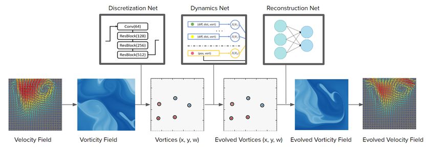
Under review as a conference paper at ICLR 2021

                                     Figure 1: System Overview

if chosen wisely, these vortices will be able to fully describe the dynamics of the original vorticity
field. Since the n × m grid will be of size around 40000 and the number of vortices k will typically
be less than 50, this precedure drastically reduces the simulation dimensionality. To view it another
way, we have created a physically-valid latent space for the dynamic simualtion to be performed on.
After the Discretization Net chooses the k vortices, the Dynamics Net will evolve these vortices
forward in time for one timestep. This Dynamics Net will be implemented by a Graph Neural
Network (GNN) with the vortices being the nodes. Such design is physically inspired by the fact that
the dynamic interaction of the vortices are analogous as in the N-body problem, which is naturally
implemented by the message passing mechanism of the GNNs. Despite that, we expect the GNN to
not merely reproduce the Biot-Savart laws for the N-body problem, but build upon that to learn more
complex, nonlinear dynamics, which is crucial as the vortex interact nonlinearly due to viscosity,
vortex stretching, solid boundary conditions and unmodelled external forces.
After the Dynamics Net evolves the (x, y) and ω of each vortex, the Reconstruction Net will map the
vortices back to the vorticity field, in order to to complete the simulation cycle. Here, we make use
of the common assumption that the vorticity in one particular spot is the summation of the influence
form each vortex on that spot. Thus, our network processes one vortex at a time. In particular, it will
take in one pair of x and ω and output a vorticity image of shape n × m, which will be summed up
for each vortex.
Finally, as ω = ∇ × u, we will be able to reconstruct the evolved velocity field from the recon-
structed vorticity field by means of integration. The evolved velocity field will then be fed back to
the system for rediscretization. As a result, our method supports the splitting and merging of vortices
dynamically.

2.3   T HREE - STAGE C URRICULUM L EARNING

Given the high dimensionality of our data and the complexity of their coupling, to train
our encode-dynamic-decode structure in an end-to-end manner is infeasible. In order to al-
leviate the training difficulty, we propose a novel, three-stage curriculum learning. The
essence of curriculum learning is to gradually increase the level of difficulty as the train-
ing session progresses, as proposed by (6). Our method of implementing such a curricu-
lum is through the generation of two datasets: separable the first, and complex the second.
In short, the separable dataset is the dataset
that we create with clear idea of where the
vortices are, i.e we randomly choose places
in space and initialize neighboring cells to
have significant vorticity; the complex dataset
is the dataset that we encounter in the wild,
where we don’t know where vortices may be.
In practice, we would want our system to per-
form in the second scenario. But directly train-

                                                   3Figure 2:   Schematics of the Two Generated
                                                    Datasets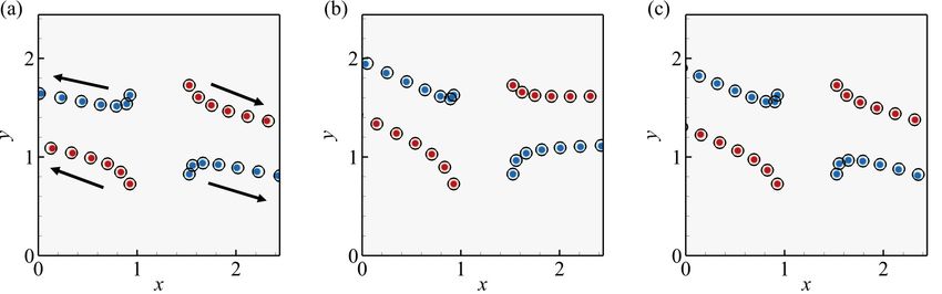
Under review as a conference paper at ICLR 2021

ing on the complex dataset leads to training
failures —— with only the initial vorticity field
(200 × 200) as input, and the evolved vorticity
field (200 × 200) as ground truth, the training
gets stuck at poor local minima, because in the
massive search space, there are so many ways
that the network can change its parameters to go downhill on the loss contour, but the one we want
is very particular —— one in which the first network would perform only discretization, the second
only dynamic evolution, and the third only spatial remapping. In such situation, we decide to pre-
fitting each network with supervised learning, taking advantage the physically legitimate assumption
that the dynamics and reconstruction networks do not care about the number of vortices there are.
Whether there are two vortices or twenty shouldn’t make a difference, because the Dynamics Net
learns the massage passing between nodes which extends naturally, while the Reconstruction Net
operates on one vortex at a time.
With that as our premise, we create the separa-
ble dataset in which we no only have the initial
and evolved field, but also the ground truth of
where the initial vortices are, as shown in Fig-
ure. 2. This enables us to pre-train the Dis-
cretization Net and the Reconstruction Net in
Stage 1 as shown in Figure. 3 using the separa-
ble data. Once we obtain the trained Discretiza-
tion Net, we are able to train the Dynamics Net.
We originally have only the initial Vortex in-
formation, but not the evolved Vortex informa-
tion, but now we are able to obtain the evolved
Vortices by running the Discretization Net on              Figure 3: Three-Stage Training Scheme
the evolved Vorticity Field, which allows us to
learn the dynamics on the Vortex domain. At this point, all three networks have been pre-trained.
Since we assume that the dynamics net and the Reconstruction Net trained on the separable dataset
can be generalized to the complex dataset, to transfer our model onto the complex dataset, we just
need to retrain the Discretization Net. Since now there is only one trainable module, we can run
gradient descent in an end-to-end manner, with loss calculated directly with the ground truth vortic-
ity field. In short, the key idea is that, we first learn and define the behaviors of the vortices using
simple data, and with these vortices as our tool, we proceed to learn to deploy these vortices with
complex data.

3     I MPLEMENTATION
3.1   DATA G ENERATION

As mentioned previously, our dataset would be obtained from the Eulerian DNS method, which
solves Equation. 3 in the periodic box using a standard pseudo-spectral method (31). Aliasing errors
are removed using the two-thirds truncation method with the maximum wavenumber kmax ≈ N/3.
The Fourier coefficients of the velocity is advanced in time using a second-order Adams–Bashforth
method, and the time step is chosen to ensure that the Courant–Friedrichs–Lewy number is less than
0.5 for numerical stability and accuracy. The pseudo-spectral method used in this DNS is similar to
that described in (40; 41; 42; 43).

3.2   D ISCRETIZATION N ET

The input of the detection networks is a vorticity field of size 200 × 200 × 1. As shown in Figure
4, we first feed the vorticity field into a small one-stage detection network and get the feature map
of size 25 × 25 × 512 (we downsampled 3 times). The primary reason for downsampling is to avoid
extremely unbalanced data and multiple prediction for the same vortex. We then forward the feature
map to 2 branches. In the first branch, we conduct a 1 × 1 convolution to generate a probability score
p̂ of the possibility that there exists a vortex. If p̂ > 0.5, we believe there exists a vortex within the
corresponding cells of the original 200 × 200 × 1 vorticity field. In the second branch, we predict

                                                    4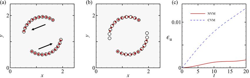
Under review as a conference paper at ICLR 2021

Figure 4: The architecture of the discretization. It takes the vorticity field as input and output the po-
sition and vortex volume for each vortex detected. The Conv means the Conv2d-BatchNorm-ReLU
combo and the ResBlock is the same as in (16). In each ResBlock, we use stride 2 to downsample
the feature map. The number in the parenthesis is the output dimension.

Figure 5: The architecture of the dynamics network. It takes the particles attribution as input and
output the position for each vortex. The ResBlock has the same architecture as in (16) with the
convolution layers replaced by linear layers. The number in the parenthesis is the output dimension.

the relative position to the left-up corner of the cell of the feature map if the cell contains a vortex.
We use the focal loss (20) to relief the unbalanced classification problem.

3.3   DYNAMICS N ET

To learn the underlying dynamics of the vortices, we build a graph neural network similar to (3).
We predict the velocity of one vortex due to influences exerted by the other vortices and the ex-
ternal force, and use the fourth-order Runge–Kutta integrator to calculate the position in the next
timestamp. As shown in Figure 5, for each vortex, we use a neural network A(θ1 ) to predict the
influences exerted by the other vortices and add them up. The input of the A(θ1 ) is the vector
(diffij , distij , vortj ) of length 4. In addition, we use another neural network A(θ2 ) to predict the
global influence caused by the external force, which is determined by the vorticity and the position
of the vortex. The input of A(θ2 ) is a vector of length 3. The output is the influence exerted by the
environment on the vortex i. Note that both the outputs of A(θ1 ) and A(θ2 ) are of length 2. The
two kinds of influence will be summed up, the result being the velocity of the vortex i. We feed the
velocity into the fourth-order Runge-Kutta integrator to obtain the predicted position of vortex i.

3.4   R ECONSTRUCTION N ET

The Reconstruction Net will be a simple small fully connected Network. Given a vortex (x, y, ω) we
want to output a 200 × 200 vorticity field. We will compute each cell 200 × 200 field independently.
Given the (x, y, ω), for each cell in the 200 × 200 grid, it computes the x-diff, y-diff, distance of that
cell. These three quantities along with the vortex’s strength will be passed into the Reconstruction
Network to output a vorticity. This process will be parallelized and can be efficiently conducted.

4     R ESULTS

4.1   L EAPFROG AND T URBULENCE

A classic example of filament dynamics are the leapfrogging vortex rings, which is an axisym-
metric laminar flow. This phenomenon is typically very hard to reproduce in standard fluid

                                                    5
Under review as a conference paper at ICLR 2021
Figure 7: Vorticity field predicted using 4 vortices under the initial condition of leapfrogging vortex
rings at t = 0, t = 11, t = 22, and t = 33. Vortices are indicated by the white–black circles. For
better visualization, we use 80000 tracers.
solver (8), especially to keep the symmetric structure. Here, we use VortexNet to predict the
motions of 4 vortices and add 80000 randomly initialized tracers for better visualization. Since
the tracers do not affect the dynamics of the underlying vorticity field, we use Biot-Savart law
to calculate the motions of these tracers for faster visualization. Figure 7 shows the evolution
of the vorticity field predicted by VortexNet under the initial condition of leapfrogging vortex
rings at t = 0, t = 11, t = 22, and t = 33. VortexNet accurately captures the sym-
metric structure of the leapfrogging vortex rings without losing such feature as time evolves.
Besides simple systems like leapfrogging vor-
tex rings, VortexNet is capable of predicting
complicated turbulence systems. Figure 6 de-
picts the two-dimensional Lagrangian scalar
fields at t = 1 with the initial condition φ = x
and resolution 20002 . The governing equation
of the Lagrangian scalar fields is
∂φ
+ u · ∇φ = 0. (1) Figure 6: Two-dimensional Lagrangian scalar
∂t
fields at t = 1 with the initial condition φ = x and
resolution 20002 . The evolution of the two La-
grangian scalar fields are induced by VortexNet.
The evolution of the Lagrangian scalar fields
are induced by O(10) and O(100) vortex par-
ticles. Based on the particle velocity field from
the VortexNet, a backward-particle-tracking
method is applied to solve equation 1, and then
the iso-contour of the Lagrangian field can be
extracted as material structures in the evolution (46; 45; 47; 49; 48).
In Figure 6 (a), the spiral structure (21; 22) of individual VortexNet vortex particles can be observed
clearly due to the small number of VortexNet vortex particles. In Figure 6 (b), the underlying field
exhibits turbulent behaviors, since it is generated with a large number of VortexNet particles. We
demonstrate that VortexNet is capable of generating an accurate depiction of complex turbulence
systems with low computational cost.
6Under review as a conference paper at ICLR 2021
Figure 8: Prediction results using VortexNet for three cases with (a) f = 0, (b) f = 0.05ω(1, 0),
and (c) f = 0.02ω(cos(x − xc ), − sin(y − yc )). The black arrows indicate the directions of the
motions of the 2 vortices. ω represents the vorticity, and (xc , yc ) is the center of the computation
domain.
Figure 9: Comparison with end-to-end trained U-Net. Left: the L2 error of vorticity field prediction
documented over 300 test trials. Middle: the aggregate L1 vorticity error field over the trials for
U-Net. Middle: the aggregate L1 vorticity error field over the trials for VortexNet. Darker color
represents higher prediction error.
4.2 E ULER EQUATIONS WITH E XTERNAL F ORCES
In Figure 8, we show Vortex’s ability of stably making accurate predictions of fluid dynamics gov-
erned by Euler equations with different external forces, which are (a) f = 0, (b) f = 0.05ω(1, 0),
and (c) f = 0.02ω(cos(x − xc ), − sin(y − yc )). ω represents the vorticity, and (xc , yc ) is the center
of the computation domain.
To prove the efficacy of our method compared to existing state-of-the-art methods, we conduct three
experiments: first, we compare our method to the End-to-End training approach using the U-net
architecture, then, we will investigate how our VortexNet method compares to the DeepHPM +
PINN approach. Lastly, we will compare our VortexNet with the conventional Vortex Method (34).
4.3 C OMPARISON WITH U- NET
In this experiment, we seek to investigate how our three-stage curriculum learning algorithm bene-
fits the learning results compared to the direct end-to-end approaches. We at first tried to train our
network architecture directly from initial and final vorticity fields, but due to the learning ambigu-
ities as conjectured previously, the training was unable to converge. Then we adopted the U-net
as proposed in (32), which provides state-of-the-art results for image semantics segmentation and
reconstruction, whose encoding-decoding structure favors our application of learning directly form
high-dimensional data. We conduct 300 test trials which we ask our network and the trained U-net
to predict the evolved vorticity field. As shown in Figure. 9, the left figure shows the scattered L2
error over the 300 trials, from which it can be concluded that our method vastly outperforms the
end-to-end trained benchmark. The same result can be seen from the other two figures, which shows
that the aggregate error outputted by the VortexNet is significantly smaller than that of the U-net.
7Under review as a conference paper at ICLR 2021
4.4 C OMPARISON WITH D EEP HPM+PINN
In this experiment, we used the same dataset that we train the VortexNet with to train the Navier-
Stokes DeepHPM model as proposed in (27). However, we realize that the DeepHPM model is
unable to converge using the data that VortexNet is trained on. This is predominantly due to the fact
that DeepHPM requires sequential data to learn the network ω(x, t), while our method trains from
snippet consisting of only two timesteps, which greatly alleviates the data requirement. Also, as
previously discussed, the DeepHPM model trains each ω(x, t) for a specific initial condition, while
our dataset shoots at a broad range of initial conditions. Our method is able to learn initial-condition
far lesser data to learn a dynamics model that is general to initial conditions than it is required for
the DeepHPM approach to do the same. In addition to comparing to DeepHPM, we also compared
our approach with the conventional vortex methods and reported the results in the Appendix A.4.
5 R ELATED WORK
Machine learning in fluid systems The rapid advent of machine learning techniques is opening up
new possibilities to solve the physical system’s identification problems by statistically exploring the
underlying structure of a variety of physical systems, encompassing applications in quantum physics
(35), thermodynamics (17), material science (36), rigid body control (12), Lagrangian systems (9),
and Hamiltonian systems (14; 19; 37). Specifically, in the field of fluid mechanics, machine learning
offers a wealth of techniques to extract information from data that could be translated into knowledge
about the underlying fluid field, as well as exhibits its ability to augment domain knowledge and
automate tasks related to flow control and optimization (7; 15). Recently, many pieces of research
are developed to efficiently learn the fluid dynamics through incorporating physical priors into the
learning framework, e.g., encoding the Navier-Stokes equations (26), embedding the notion of an
incompressible fluid (24), and identifying a mapping between the dynamics of wave-based physical
phenomena and the computation in a recurrent neural network (RNN) (18).
Learning physics laws from high dimensional observations One of the key strengths of neural
networks is that they can learn abstract representations directly from high-dimensional data such
as pixels. With the advances of image detection techniques (16; 30), it is natural to apply these
techniques to better learn and predict physical phenomena. Belbute-Peres et al., attempted to learn
a model of physical system dynamics end-to-end from image sequences using an autoencoder (4).
Greydanus et al., also tried to combine an autoencoder with an Hamiltonian Neural Networks (HNN)
to model the dynamics of pixel observations of a pendulum (14). Toth et al., later developed Hamil-
tonian Generative Network (HGN), which is capable of consistently learning Hamiltonian dynamics
from high-dimensional observations without restrictive domain assumptions (38). Some related
works done on fluid dynamics include Hidden Fluid Mechanics (HFM) by Raissi et al., (28). How-
ever, HFM differs from our work by learning the underlying governing function purely based on the
Eulerian grid.
6 C ONCLUSION
In this paper, we present a novel physics-based network structure that facilitates the learning of
complex dynamic systems. Inspired by the Vortex Method in fluid dynamics, our method creates a
physically-legitimate latent space for fast and realistic simulation of complex, unsteady fluid flows.
We enforce a Lagrangian discretization with a Encoder—Dynamics—Decoder network structure,
and train it with a novel three-stage curriculum learning algorithm, while keeping the physical fi-
delity by training with data generated from the high precision Eulerian DNS method. Our method
fundamentally differs from the current approaches in the field of physics-informed learning, because
instead of tailoring our network to learn the governing PDEs, we design our network architecture
to describe the underlying structures these equations imply. We show that our method provides
superior results to previous approaches, for being more versatile, general to initial conditions and
yielding more physical-correctness with less data sample. Our method opens up a new frontier for
embedding knowledge prior via constructing physics-driven latent spaces, which can be inspiring to
research areas well beyond physical simulation.
8Under review as a conference paper at ICLR 2021
R EFERENCES
[1] JS Anderson, IG Kevrekidis, and R Rico-Martinez. A comparison of recurrent training algo-
rithms for time series analysis and system identification. Computers & chemical engineering,
20:S751–S756, 1996.
[2] Lorena A Barba. Vortex Method for computing high-Reynolds number flows: Increased accu-
racy with a fully mesh-less formulation. PhD thesis, California Institute of Technology, 2004.
[3] P. Battaglia, R. Pascanu, M. Lai, and D. J. Rezende. Interaction networks for learning about
objects, relations and physics. In Advances in neural information processing systems, pages
4502–4510, 2016.
[4] de A. F. Belbute-Peres, A. K. Smith, K. Allen, J. Tenenbaum, and Z. J. Kolter. End-to-end
differentiable physics for learning and control. In Advances in neural information processing
systems, pages 7178–7189, 2018.
[5] Filipe de Avila Belbute-Peres, Thomas D Economon, and J Zico Kolter. Combining dif-
ferentiable pde solvers and graph neural networks for fluid flow prediction. arXiv preprint
arXiv:2007.04439, 2020.
[6] Yoshua Bengio, Jérôme Louradour, Ronan Collobert, and Jason Weston. Curriculum learning.
In Proceedings of the 26th annual international conference on machine learning, pages 41–48,
2009.
[7] S. L. Brunton, B. R. Noack, and P. Koumoutsakos. Machine Learning for Fluid Mechanics.
Annu. Rev. Fluid Mech., 52:477–508, 2020.
[8] A. Chern, F. Knöppel, U. Pinkall, P. Schröder, and S. Weißmann. Schrödinger’s smoke. ACM
Trans. Graph., 35:77, 2016.
[9] M. Cranmer, S. Greydanus, S. Hoyer, P. Battaglia, D. Spergel, and S. Ho. Lagrangian neural
networks. arXiv:2003.04630, 2020.
[10] James P Crutchfield and Bruce S McNamara. Equations of motion from a data series. Complex
systems, 1(417-452):121, 1987.
[11] Bryan C Daniels and Ilya Nemenman. Automated adaptive inference of phenomenological
dynamical models. Nature communications, 6(1):1–8, 2015.
[12] Z. Geng, D. Johnson, and R. Fedkiw. Coercing machine learning to output physically accurate
results. J. Comput. Phys., 406:109099, 2020.
[13] Raul González-Garcı́a, Ramiro Rico-Martı́nez, and Ioannis G Kevrekidis. Identification of dis-
tributed parameter systems: A neural net based approach. Computers & chemical engineering,
22:S965–S968, 1998.
[14] S. Greydanus, M. Dzamba, and J. Yosinski. Hamiltonian neural networks. In Advances in
Neural Information Processing Systems, pages 15379–15389, 2019.
[15] Philipp H., Nils T., and Vladlen K. Learning to Control PDEs with Differentiable Physics. In
International Conference on Learning Representations, 2020.
[16] K. He, X. Zhang, S. Ren, and J. Sun. Deep residual learning for image recognition. In Pro-
ceedings of the IEEE conference on computer vision and pattern recognition, pages 770–778,
2016.
[17] Q. Hernandez, A. Badias, D. Gonzalez, F. Chinesta, and E. Cueto. Structure-preserving neural
networks. arXiv:2004.04653, 2020.
[18] T. W. Hughes, I. A. D. Williamson, M. Minkov, and S. Fan. Wave physics as an analog
recurrent neural network. Sci. Adv., 5:6946, 2019.
[19] P. Jin, A. Zhu, G. E. Karniadakis, , and Y. Tang. Symplectic networks: Intrinsic structure-
preserving networks for identifying Hamiltonian systems. arXiv:2001.03750, 2020.
9Under review as a conference paper at ICLR 2021
[20] T. Lin, P. Goyal, R. Girshick, K. He, and P. Dollár. Focal loss for dense object detection. IEEE
Trans. Vis. Comput. Graph., pages 2980–2988, 2017.
[21] T. S. Lundgren. Strained spiral vortex model for turbulent fine structure. Phys. Fluids,
25:2193–2203, 1982.
[22] T. S. Lundgren. A small-scale turbulence model. Phys. Fluids A, 5:1472, 1993.
[23] Kjetil O Lye, Siddhartha Mishra, and Deep Ray. Deep learning observables in computational
fluid dynamics. Journal of Computational Physics, page 109339, 2020.
[24] A. T. Mohan, N. Lubbers, D. Livescu, and M. Chertkov. Embedding hard physical constraints
in convolutional neural networks for 3D turbulence. In International Conference on Learning
Representations, 2020.
[25] Arvind T Mohan, Nicholas Lubbers, Daniel Livescu, and Michael Chertkov. Embedding
hard physical constraints in neural network coarse-graining of 3d turbulence. arXiv preprint
arXiv:2002.00021, 2020.
[26] M. Raissi and G. E. Karniadakis. Hidden physics models: Machine learning of nonlinear
partial differential equations. J. Comput. Phys., 357:125–141, 2018.
[27] M. Raissi, P. Perdikaris, and G. E. Karniadakis. Physics-informed neural networks: A deep
learning framework for solving forward and inverse problems involving nonlinear partial dif-
ferential equations. J. Comput. Phys., 378:686–707, 2019.
[28] M. Raissi, A. Yazdani, and G. E. Karniadakis. Hidden fluid mechanics: Learning velocity and
pressure fields from flow visualizations. Science, 367(6481):1026–1030, 2020.
[29] Maziar Raissi, Paris Perdikaris, and George Em Karniadakis. Multistep neural networks
for data-driven discovery of nonlinear dynamical systems. arXiv preprint arXiv:1801.01236,
2018.
[30] J. Redmon, S. Divvala, R. Girshick, and A. Farhadi. You only look once: Unified, real-
time object detection. In Proceedings of the IEEE conference on computer vision and pattern
recognition, pages 779–788, 2016.
[31] R. S. Rogallo. Numerical experiments in homogeneous turbulence. In Technical Report
TM81315, NASA, 1981.
[32] Olaf Ronneberger, Philipp Fischer, and Thomas Brox. U-net: Convolutional networks for
biomedical image segmentation. In International Conference on Medical image computing
and computer-assisted intervention, pages 234–241. Springer, 2015.
[33] Samuel H Rudy, Steven L Brunton, Joshua L Proctor, and J Nathan Kutz. Data-driven discov-
ery of partial differential equations. Science Advances, 3(4):e1602614, 2017.
[34] A. Selle, N. Rasmussen, and R. Fedkiw. A vortex particle method for smoke, water and explo-
sions. ACM Trans. Graph., 3:910–914, 2005.
[35] J. M. Sellier, G. M. Caron, and J. Leygonie. Signed particles and neural networks, towards
efficient simulations of quantum systems. J. Comput. Phys., 387:154–162, 2019.
[36] G. H. Teicherta, A. R. Natarajanc, A. Van der Venc, and K. Garikipati. Machine learning ma-
terials physics: Integrable deep neural networks enable scale bridging by learning free energy
functions. Comput. Methods Appl. Mech. Engrg., 353:201–216, 2019.
[37] Y. Tong, S. Xiong, X. He, G. Pan, and Bo Z. Symplectic neural networks in Taylor series form
for Hamiltonian systems, 2020.
[38] P. Toth, D. J. Rezende, A. Jaegle, S. Racanière, A. Botev, and I. Higgins. Hamiltonian genera-
tive networks. In International Conference on Learning Representations, 2020.
[39] Cristina White, Daniela Ushizima, and Charbel Farhat. Neural networks predict fluid dynamics
solutions from tiny datasets. arXiv preprint arXiv:1902.00091, 2019.
10Under review as a conference paper at ICLR 2021
[40] S. Xiong and Y. Yang. The boundary-constraint method for constructing vortex-surface fields.
J. Comput. Phys., 339:31–45, 2017.
[41] S. Xiong and Y. Yang. Construction of knotted vortex tubes with the writhe-dependent helicity.
Phys. Fluids, 31:047101, 2019.
[42] S. Xiong and Y. Yang. Identifying the tangle of vortex tubes in homogeneous isotropic turbu-
lence. J. Fluid Mech., 874:952–978, 2019.
[43] S. Xiong and Y. Yang. Effects of twist on the evolution of knotted magnetic flux tubes. J. Fluid
Mech., 895:A28, 2020.
[44] XIA Yang, S Zafar, J-X Wang, and H Xiao. Predictive large-eddy-simulation wall modeling
via physics-informed neural networks. Physical Review Fluids, 4(3):034602, 2019.
[45] Y. Yang and D. I. Pullin. Geometric study of Lagrangian and Eulerian structures in turbulent
channel flow. J. Fluid Mech., 674:67–92, 2011.
[46] Y. Yang, D. I. Pullin, and I. Bermejo-Moreno. Multi-scale geometric analysis of Lagrangian
structures in isotropic turbulence. J. Fluid Mech., 654:233–270, 2010.
[47] Y. Zhao, Y. Yang, and S. Chen. Evolution of material surfaces in the temporal transition in
channel flow. J. Fluid Mech., 793:840–876, 2016.
[48] W. Zheng, S. Ruan, Y. Yang, L. He, and S. Chen. Image-based modelling of the skin-friction
coefficient in compressible boundary-layer transition. J. Fluid. Mech., 875:1175–1203, 2019.
[49] W. Zheng, Y. Yang, and S. Chen. Evolutionary geometry of Lagrangian structures in a transi-
tional boundary layer. Phys. Fluids, 28:035110, 2016.
A F LUID M ECHANICS BACKGROUND
A.1 T HE NAVIER -S TOKES E QUATION
The Navier-Stokes Equation is the governing equation for Newtonian Fluids. It generally comes
in two different forms, first of which is the more commonly known, Velocity-Pressure Form, also
called the Primitive Variable Form:
∂u 1
+ (u · ∇)u = − ∇p + v∇2 u + f , ∇ · u = 0, (2)
∂t ρ
where u is the velocity vector, ρ the density, p the pressure and f the extermal force. This equation
can be solved numerically on Eulerian grids using finite difference. To directly compute ∂u ∂t and
perform temporal evolution on u is a common strategy, referred to as the Direct Numerical Simu-
lation (DNS) methods, which is a fundamentally Eulerian approach. The advantage of this method
is its physical fidelity, but it also has several drawbacks: First, the Eulerian grid-based approach
inevitably suffers from numeric dissipation, which makes it impotent when it comes to modelling
complex and unsteady flows (2). Secondly, since the simulation domain is confined by the grids,
this method struggles when performing free-space simulation. And even more importantly, solving
such PDEs on the grid is computationally expensive, which would become outrageously so as we
push towards high precision.
A.2 VORTEX M ETHOD
The alternative form of the Navier-Stokes equation might be obtained by defining the vorticity ω =
∇ × u, which leads to the following velocity-vorticity form.
Dω
= (ω · ∇)u + v∇2 ω + ∇ × B (3)
Dt
where ω is the vorticity, u is the velocity and B the external force field. Although this form does
not seem to bring any simplification, the key illumination of doing this transformation stems the
11Under review as a conference paper at ICLR 2021
Helmholtz’s theorems, which states that the dynamics of the vorticity field can be described by
vortex elements, who are Lagrangian particles flowing with the velocity field (2). To gain some
more intuition into the significance of this, think about a lake where complex fluid motion occurs
everywhere. To learn a function to describe what’s happening in every cubic centimeter in the lake
is going to be a monstrous task. What the Helmholtz’s theorem is telling us, is that all of these things
that are happening can be fully accredited to a small number of invisible agitators flowing with the
field. So rather than trying to do the former, we can alternatively do the following: locate these
invisible agitators and then predict how these agitators interact and move over time.
This is exactly the idea behind the Vortex method. In this method, the space is discretized not into
Eulerian grids, but into a number of Lagrangian particles —— the vortices. Each vortex carries
with it a strength, using which we will be able to fully reconstruct the velocity field. Since these
vortices are Lagrangian particles, their movements are determined by the velocity field that they
themselves create, thus allowing us to advance the simulation temporally. The obvious benefit of
this method is that, since there will be much lesser Lagrangian vortices than there are Eulerian grid
nodes, to simulate only on these vortices is a process extremely efficient computation-wise. Besides,
this method enjoys the advantage of being adaptable to arbitrary precision, trivially handling open-
space boundary conditions, free from numeric dissipation, and it automatically preserves circulation
which makes it great for modelling complex and unsteady flows. However, its drawback is the
lack of physical integrity, which is largely due to the amount of human heuristics required in its
procedure. For instance, the very definition of a vortex varies from paper to paper, it can be a point,
a fixed blob or a deformable blob. It is up to each researcher to decide how to deploy these vortices
given a vorticity field, how these vortices interact with one another, how they split up and merge
together, and etc., where some painfully elaborate algorithms had to be used. Secondly, the Vortex
method, unlike Eulerian methods, is inconvenient for adding in viscous diffusion, solid boundary
conditions, or external forces. When these traits are the desired, researchers develop a large number
of techniques to make the simulation results look more realistic, which at the mean time make the
method much less implementable and less elegant. Since these methods are not physics-based, they
provide visually appealing, but not physically realistic results.
B C OMPARISON WITH THE VORTEX M ETHOD
To demonstrate that VortexNet is a better approach to capture the fluid dynamics than the traditional
methods, we compare the prediction results made by VortexNet and conventional Vortex Method for
solving Euler equations in the periodic box. We plot the results using VortexNet and conventional
Vortex Method, and the relative error of velocity in the simulation in Figure 10 (a), (b), and (c)
respectively. The red dots indicate the positions of 2 vortices at different time steps generated by
DNS, and the black circles are the prediction results of VortexNet and conventional Vortex Method.
It is quite obvious that in Figure 10 (a) the predictions made by VortexNet match the positions of
vortices generated by DNS almost perfectly, while the predictions made by BS law in Figure 10
(b) contain a large error. The divergence of the relative error of velocity shown in Figure 10 (c)
as t increases also shows that VortexNet outperformances the traditional methods by an increasing
amount as the predicting period becomes longer.
12Under review as a conference paper at ICLR 2021
Figure 10: Comparison of VortexNet and conventional Vortex Method for solving Euler equation
in the periodic box. (a) VortexNet, (b) conventional Vortex Method, and (c) The relative error of
velocity in flow simulation. The red dots indicate the positions of 2 vortices at different time steps
generated by DNS, and the black-circles in (a) and (b) are the prediction results of VortexNet and
conventional Vortex Method, respectively. The black arrows indicate the directions of the motions
of the 2 vortices.
13You can also read