Efficient Differentiable Simulation of Articulated Bodies
←
→
Page content transcription
If your browser does not render page correctly, please read the page content below
Efficient Differentiable Simulation of Articulated Bodies

                            Yi-Ling Qiao * 1 2 Junbang Liang * 1 Vladlen Koltun 2 Ming C. Lin 1

                           Abstract                              2019). However, they do not have access to analytic deriva-
                                                                 tives of the articulated dynamics. Therefore, nearly all
        We present a method for efficient differentiable         gradient-based approaches have to design strategies to com-
        simulation of articulated bodies. This enables in-       pute the gradients indirectly when dealing with articulated
        tegration of articulated body dynamics into deep         bodies.
        learning frameworks, and gradient-based opti-
        mization of neural networks that operate on ar-          The straightforward way to differentiate the simulation is
        ticulated bodies. We derive the gradients of the         to use existing automatic differentiation tools (Griewank &
        contact solver using spatial algebra and the adjoint     Walther, 2008; Abadi et al., 2016; Paszke et al., 2019). How-
        method. Our approach is an order of magnitude            ever, autodiff tools consume prohibitive amounts of memory
        faster than autodiff tools. By only saving the ini-      when there are many simulation steps. Autodiff tracks every
        tial states throughout the simulation process, our       operation and stores the intermediate results in order to per-
        method reduces memory requirements by two or-            form backpropagation. In articulated body simulation, the
        ders of magnitude. We demonstrate the utility of         iterative contact solver and the dynamics algorithm (Feath-
        efficient differentiable dynamics for articulated        erstone, 2007) yield exceedingly long computational graphs.
        bodies in a variety of applications. We show that        In our experiments, differentiable simulators built with au-
        reinforcement learning with articulated systems          todiff tools run out of memory after 5,000 simulation steps –
        can be accelerated using gradients provided by           just a few seconds of experience. As a result, learning is
        our method. In applications to control and inverse       constrained to short experiences or forced to used large time
        problems, gradient-based optimization enabled by         steps, thus curtailing the scope of behaviors that can be
        our work accelerates convergence by more than            learned or undermining the simulation’s stability.
        an order of magnitude.                                   Furthermore, the overhead of creating and storing the aux-
                                                                 iliary variables for autodiff also slows down the forward
                                                                 simulation. Although autodiff tools like DiffTaichi (Hu
1. Introduction                                                  et al., 2020) and JAX (Bradbury et al., 2018) can accelerate
                                                                 the simulation of fluids and deformable solids by vectoriza-
Differentiable physics enables efficient gradient-based opti-
                                                                 tion, it is difficult to achieve the same speedup in articulated
mization with dynamical systems. It has achieved promising
                                                                 body simulation because the articulated dynamics algorithm
results in both simulated (Hu et al., 2019; Qiao et al., 2020)
                                                                 is highly serialized, unlike inherently parallel computation
and real environments (Bern et al., 2019; Song & Boularias,
                                                                 on grids and particles.
2020a). Our goal is to make articulated body simulation
efficiently differentiable. We aim to maximize efficiency in     In this paper, we design a differentiable articulated body sim-
both computation and memory use, in order to support fast        ulation method that runs 10x faster with 1% of the memory
gradient-based optimization of differentiable systems that       consumption compared to differentiation based on autodiff
interact with articulated bodies in physical environments.       tools. In order to minimize the overhead of differentiation,
                                                                 we derive the gradients of articulated body simulation us-
Articulated bodies play a central role in robotics, computer
                                                                 ing the adjoint method (Giles & Pierce, 2000). The adjoint
graphics, and embodied AI. Many control systems are op-
                                                                 method has been applied to fluids (McNamara et al., 2004)
timized via experiences collected in simulation (Todorov
                                                                 and multi-body systems (Geilinger et al., 2020), but these
et al., 2012; Coumans, 2015; Lee et al., 2018; Tedrake et al.,
                                                                 applications do not support physically correct differentiable
    *
    Equal contribution 1 University of Maryland, College Park    simulation of articulated bodies. Our derivation of the oper-
2
 Intel Labs. Correspondence to: Yi-Ling Qiao, Junbang Liang,     ator adjoints uses spatial algebra (Featherstone, 2008). Our
and Ming C. Lin , Vladlen      method needs almost no additional computation during the
Koltun .
                                                                 forward simulation and is an order of magnitude faster than
Proceedings of the 38 th International Conference on Machine     autodiff tools.
Learning, PMLR 139, 2021. Copyright 2021 by the author(s).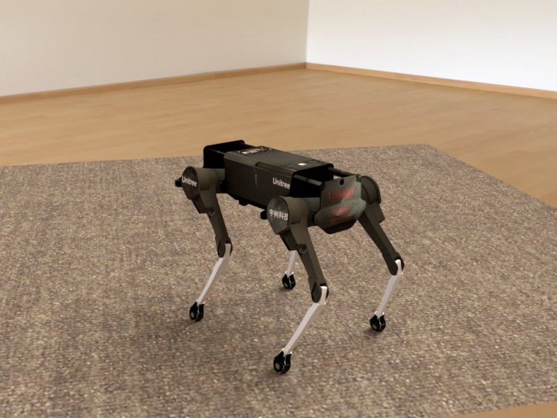
Efficient Differentiable Simulation of Articulated Bodies

We further reduce memory requirements by adapting ideas           volve physical systems. Degrave et al. (2019) advocate using
from checkpointing (Griewank & Walther, 2000; Chen et al.,        differentiable physics to solve control problems in robotics.
2016) to the differentiable simulation setting. In the forward    de Avila Belbute-Peres et al. (2018) obtain gradients of 2D
pass, we store the initial simulation state for each time step.   rigid body dynamics. Liang et al. (2019) use automatic
During backpropagation, we recreate intermediate variables        differentiation tools to obtain gradients for cloth simulation.
by reproducing simulation from the stored state. The overall      Qiao et al. (2020) develop a more comprehensive differen-
runtime remains fast, while memory consumption is reduced         tiable physics engine for rigid bodies and cloth based on
by two orders of magnitude.                                       mesh representations. Ingraham et al. (2019) present dif-
                                                                  ferentiable simulation of protein dynamics. For volumetric
As an application of differentiable dynamics for articulated
                                                                  data, ChainQueen (Hu et al., 2019) computes gradients of
systems, we show that reinforcement learning (RL) can ben-
                                                                  the MPM simulation pipeline. Bern et al. (2019) use FEM
efit from the knowledge of gradients in two ways. First, it
                                                                  to model soft robots and perform trajectory optimization
can make use of the gradients computed by the simulation to
                                                                  with analytic gradients. Takahashi et al. (2021) differentiate
generate extra samples using first-order approximation. Sec-
                                                                  the simulation of fluids with solid coupling.
ond, during the policy learning phase, differentiable physics
enables us to perform a one-step rollout of the objective         Many exciting applications of differentiable physics have
value function so that the policy updates can be more ac-         been explored (Spielberg et al., 2019; Heiden et al., 2019;
curate. Both schemes effectively improve the convergence          2020; Wang et al., 2020; Krishna Murthy et al., 2021).
speed and the attained reward. We also demonstrate ap-            Huang et al. (2021) propose a soft-body manipulation bench-
plications of efficient differentiable articulated dynamics       mark for differentiable physics. Toussaint et al. (2018) ma-
to inverse problems, such as motion control and param-            nipulate tools with the help of differentiable physics. Song &
eter estimation. Gradient-based optimization enabled by           Boularias (2020b) perform system identification by learning
our method accelerates convergence in these settings by           from the trajectory, and Song & Boularias (2020a) then use
more than an order of magnitude. Code is available on our         the estimated frictional properties to help robotic pushing.
project page: https://github.com/YilingQiao/
                                                                  A related line of work concerns the development of powerful
diffarticulated
                                                                  automatic differentiation tools that can be used to differen-
The contributions of this work are as follows:                    tiate simulation. DiffTaichi (Hu et al., 2020) provides a
                                                                  new programming language and a compiler, enabling the
   • We derive the adjoint formulations for the entire ar-
                                                                  high-performance Taichi simulator to compute the gradi-
     ticulated body simulation workflow, enabling a 10x
                                                                  ents of the simulation. JAX MD (Schoenholz & Cubuk,
     acceleration over autodiff tools.
                                                                  2020) makes use of the JAX autodiff library (Bradbury
   • We adapt the checkpointing method to the structure of
                                                                  et al., 2018) to differentiate molecular dynamics simulation.
     articulated body simulation to reduce memory con-
                                                                  These works have specifically made use of vectorization on
     sumption by 100x, making stable collection of ex-
                                                                  both CPU and GPU to achieve high performance on grids
     tended experiences feasible.
                                                                  and particle sets, where the simulation is intrinsically par-
   • We introduce two general schemes for accelerating
                                                                  allel. In contrast, the simulation of articulated bodies is far
     reinforcement learning using differentiable physics.
                                                                  more serial, as dynamics propagates along kinematic paths
   • We demonstrate the utility of differentiable simulation
                                                                  rather than acting in parallel on grid cells or particles.
     of articulated bodies in motion control and parameter
     estimation, enhancing performance in these scenarios         TinyDiffSim (Coumans et al., 2020) provides a templatized
     by more than an order of magnitude.                          simulation framework that can leverage existing autodiff
                                                                  tools such as CppAD (Bell et al., 2018), Ceres (Agarwal
2. Related Work                                                   et al., 2010), and PyTorch (Paszke et al., 2019) to differen-
                                                                  tiate simulation. However, these methods introduce signif-
Differentiable programming has been applied to render-            icant overhead in tracing the computation graph and accu-
ing (Li et al., 2018a; Nimier-David et al., 2019; Laine et al.,   mulate substantial computational and memory costs when
2020), image processing (Li et al., 2020; 2018b), SLAM (Kr-       applied to articulated bodies.
ishna Murthy et al., 2020), and design (Du et al., 2020).
                                                                  Our method does not need to store the entire computation
Making complex systems differentiable enables learning
                                                                  graph to compute the gradients. We store the initial states of
and optimization using gradient-based methods. Our liter-
                                                                  each simulation step and reproduce the intermediate results
ature review focuses on differentiable physics, the adjoint
                                                                  when needed by the backward pass. This checkpointing
method, and neural approximations of physical systems.
                                                                  strategy is also used in training neural ODEs (Zhuang et al.,
Differentiable physics. Differentiable physics provides           2020) and large neural networks (Chen et al., 2016; Gruslys
gradients for learning, control, and inverse problems that in-    et al., 2016; Kirisame et al., 2021; Shah et al., 2021). We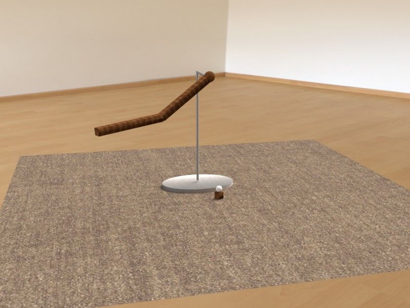
Efficient Differentiable Simulation of Articulated Bodies
are the first to adapt this technique to articulated dynamics, f = [f 1 , f 2 , ..., f nt ] = 0. For a learning or optimization
achieving dramatic reductions in memory consumption and problem, we would usually define a scalar objective
enabling stable simulation of long experiences. function Φ(x, u). To get the derivative of this function w.r.t.
the control input u, one needs to compute
Adjoint method. The adjoint method has been applied to
dΦ ∂Φ ∂Φ dx
fluid control (McNamara et al., 2004), PDEs (Holl et al., = + . (1)
2020), light transport simulation (Nimier-David et al., 2020), du ∂u ∂x du
∂Φ
and neural ODEs (Chen et al., 2018; Zhuang et al., 2020). ∂u is easy to compute for each single simulation step. But
Recently, Geilinger et al. (2020) proposed to use the adjoint it is prohibitively expensive to directly solve ∂Φ dx
∂x du because
method in multi-body dynamics. However, they operate dx
du will be a 2nq nt × nq nt matrix.
in maximal coordinates and model body attachments using
springs. This does not enforce physical validity of articu- Instead, we differentiate the dynamics f (x, u) = 0 and
∂f dx ∂f
lated bodies. In contrast, we operate in reduced coordinates obtain the constraint ∂x du = − ∂u . Applying the adjoint
∂Φ dx
and derive the adjoints for the articulated body algorithm method (Giles & Pierce, 2000), ∂x du equals to
and spatial algebra operators that properly model the body’s > >
> ∂f ∂f ∂Φ
joints. This supports physically correct simulation with joint −R such that R= (2)
∂u ∂x ∂x
torques, limits, Coriolis forces, and proper transmission of
internal forces between links. Since the dynamics equation for one step only involves a
∂f ∂f
small number of previous steps, the sparsity of ∂u and ∂x
Neural approximation. A number of works approximate makes it easier to solve for the variable R in Eq. 2.
physics simulation using neural networks (Battaglia et al.,
2016; Chang et al., 2017; Mrowca et al., 2018; Schenck &
∂Φ
∂u − R> ∂u∂f
is called the adjoint of u and is equivalent to
Fox, 2018; Sanchez-Gonzalez et al., 2018; 2020; Li et al., the gradient by our substitution. In the following derivation,
2019; Belbute-Peres et al., 2020; Ummenhofer et al., 2020; we denote the adjoint of a variable s by s, and the adjoint of
Wandel et al., 2021; Pfaff et al., 2021). Physical princi- a function f (·) by f (·).
ples have also been incorporated in the design of neural
networks (Schütt et al., 2017; Anderson et al., 2019; Bo- 4. Efficient Differentiation
gatskiy et al., 2020; Chen et al., 2020; Cranmer et al., 2020).
Approximate simulation by neural networks is naturally dif- In this section, we introduce our algorithm for the gradient
ferentiable, but the networks are not constrained to abide computation in articulated body simulation. For faster dif-
by the underlying physical dynamics and simulation fidelity ferentiation, the gradients of articulated body dynamics are
may degenerate outside the training distribution. computed by the adjoint method. We derive the adjoint of
time integration, contact resolution, and forward dynamics
in reverse order. We then adapt the checkpoint method to
3. Preliminaries articulated body simulation to reduce memory consumption.
Articulated body dynamics. For the forward simula-
4.1. Adjoint Method for Articulated Dynamics
tion, we choose the recursive Articulated Body Algorithm
(ABA) (Featherstone, 2007), which has O(n) complexity One forward simulation step can be split into five modules,
and is widely used in articulated body simulators (Todorov as shown in Figure 1: perform the forward kinematics from
et al., 2012; Coumans, 2015; Lee et al., 2018). In each the root link to the leaf links, update the forces from the
simulation step k, the states xk of the system consist of leaves to the root, update the accelerations from the root
configurations in generalized coordinates and their veloc- to the leaves, detect and resolve collisions, and perform
ities xk = [qk , q̇k ] ∈ R2nq ×1 , where nq is the number of time integration. Backpropagation proceeds through these
degrees of freedom in the system. Assuming each joint can modules in reverse order.
be actuated by a torque, there is an nq -dimensional control
signal uk ∈ Rnq ×1 . The discretized dynamics at this step Time integration. Backpropagation starts from the time
can be written as f k+1 (uk , xk , xk+1 ) = 0. integration. As an example, for a simulation sequence with
nt = 3 steps and an integrator with a temporal horizon of
∂f > >
Adjoint method. We can concatenate 2, the constraints ( ∂x ) R = ( ∂Φ∂x ) in Equation 2 can be
the states in the entire time sequence into expanded as
x = [x1 , x2 , ..., xnt ] ∈ Rnt ·2nq ×1 , with correspond-
∂f 1 > ∂f 2 >
∂Φ >
ing control input u = [u1 , u2 , ..., unt ] ∈ Rnt ·nu ×1 , where ( ∂x 1) ( ∂x 1) 0 R1 ( ∂x1 )
2 3 ∂Φ >
0 ∂f >
( ∂x 2)
∂f >
( ∂x 2) R2 = ( ∂x 2)
nt is the number of simulation steps. The concate-
3
∂f 3 > R ∂Φ >
nated dynamics equations can be similarly written as 0 0 ( ∂x3 ) ( ∂x3)
(3)
Efficient Differentiable Simulation of Articulated Bodies
checkpoints Intermediate results
positions, articulated momentum,
transformations articulated inertias, body accelerations, new
states states
velocities, etc. torques, etc joint accelerations
collision
detection time
+
LCP solver
integration
update update update collision
kinematics forces accelerations resolving
Figure 1. The workflow of a simulation step. Assume there are nq = 6 DoF. The initial state is an nq × 3 matrix containing the position,
velocity, and control input of each joint. The forward dynamics will traverse the articulated body sequentially three times. This process is
difficult to parallelize and will generate a large
positions,
number of intermediate results. After the forward dynamics there is a collision resolution
articulated momentum,
step with collision detection and an iterativearticulated
transformations Gauss-Seidel
inertias,solver. body
Theaccelerations,
size of the initial state (position, velocity, and control
new input) is
states states
much smaller than that ofvelocities,
intermediate
etc. results buttorques, etc
the initial state has allaccelerations
joint the information to resume all the intermediate variables.
collision
∂f k
Forward dynamics. Our detection time simulator prop-
articulated body
If using the explicit Euler integrator, we have ∂x k = I. +
nt ∂Φ k
Initially R = ∂xnt . The following R can be computed agates the forward dynamics integration
LCP solveras shown in the green blocks
iteratively by of Figure 1. Each operation in the forward simulation has
its corresponding adjoint operation in the backward pass.
collision
update
k+1 update update
∂Φ ∂f To compute the gradients,
resolvingwe derive adjoint rules for the
Rk = ( k )> −( kinematics
)> Rk+1 , k = 1, 2,
forces
.., nt −1. (4) accelerations
∂x ∂xk operators in spatial algebra (Featherstone, 2008).
When Rk backpropagates through time, the gradients uk As a simple example, a spatial vector pi = [w, v] ∈ R6
can also be computed by Equation 2. In fact, by the way we representing the bias force of the i-th link is the sum of
calculate Rk , it equals the gradients of xk . Other parameters an external force [f1 , f2 ] ∈ R6 and a cross product of two
can also be computed in a similar way as uk . spatial motion vectors [w1 , v1 ], [w2 , v2 ] ∈ R6 :
w f1 + w1 × w2 + v1 × v2
Collision resolution. The collision resolution step consists = . (6)
v f2 + w1 × v2
of collision detection and a collision solver. Upon receiving
the gradients x from the time integrator, the collision solver Once we get the adjoint [w, v] of pi = [w, v], we can
needs to pass the gradients to detection, and then to the propagate it to its inputs:
forward dynamics. In our collision solver, we construct a
w1
−w× w2 − v× v2
Mixed Linear Complementarity Problem (MLCP) (Stepien, =
v1 −w× v2
2013): (7)
w2 w × w1 f1 w
= , =
a = Ax + b v2 w × v 1 + v × w1 f2 v
(5)
s.t. 0 ≤a ⊥ x ≥ 0 and c− ≤ x ≤ c+ , This example shows the adjoint of one forward operation.
The time and space complexity of the original operation
where x is the new collision-free state, A is the iner- and its adjoint are the same as the forward simulation. The
tial matrix, b contains the relative velocities, and c− , c+ supplement provides more details on the adjoint operations.
are the lower bound and upper bound constraints, respec-
tively. We use the projected Gauss-Seidel (PGS) method
4.2. Checkpointing for Articulated Dynamics
to solve this MLCP. This iterative solve trades off accu-
racy for speed such that the constraints a> x = 0 might not The input and output variables of one simulation step have
hold on termination. In this setting, where the solution is relatively small dimensionalities (positions, velocities, and
not guaranteed to satisfy constraints, implicit differentia- accelerations), but many more intermediate values are com-
tion (de Avila Belbute-Peres et al., 2018; Liang et al., 2019; puted during the process. Although this is not a bottleneck
Qiao et al., 2020) no longer works. Instead, we design a re- for forward simulation because the memory allocation for
verse version of the PGS solver using the adjoint method to intermediate results can be reused across time steps, it be-
compute the gradients. Further details are in the supplement. comes a problem for differentiable simulation, which needs
In essence, the solver mirrors PGS, substituting the adjoints to store the entire computation graph for the backward pass.
for the original operators. This step passes the gradients This causes memory consumption to explode when simu-
from the collision-free states to the forward dynamics. lation proceeds over many time steps, as is the case when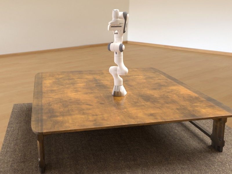
Efficient Differentiable Simulation of Articulated Bodies

                                                          forward/resume          step:
                                                          backward
         store
      checkpoints                 forward simulation                                                  Zk       = G(xk−1 ),                     (9)
                                                                                                                       k
                                                                                                      Zk       = F (Z      , xk ),            (10)
                    Forward         Collision                Time
                    Dynamics        Resolving             Integration                               xk−1       = G(xk−1      , Zk ).          (11)

        reload                                                                    5. Reinforcement Learning
      checkpoints              backward differentiation
                                                                                  Our method can be applied to simulation-based reinforce-
                    Forward         Collision                Time                 ment learning (RL) tasks to improve policy performance as
                    Dynamics        Resolving             Integration             well as convergence speed. By computing gradients with
                                                                                  respect to the actions, differentiable simulation can provide
                                                                                  more information about the environment. We suggest two
Figure 2. Differentiation of articulated body dynamics. Top:                      approaches to integrating differentiable physics into RL.
forward simulation at step k. The simulator stores the states qk , q̇k ,
and control input uk . Bottom: During backpropagation, the check-                 Sample enhancement. We can make use of the computed
points are reloaded and the simulator runs one forward step to                    gradients to generate samples in the neighborhood around an
reconstruct the intermediate variables. Beginning with the gradi-                 existing sample. Specifically, given a sample (s, a0 , s00 , r0 )
ents from step k + 1, we use the adjoint method to sequentially                   from the history, with observation s, action a0 , next-step
compute the gradients of all variables through time integration, the              observation s00 , and reward r0 , we can generate new samples
constraint solver, and forward dynamics.                                          (s, ak , s0k , rk ) using first-order approximation:

                                                                                                    ak     =     a0 + ∆ak ,
small time steps are needed for accuracy and stability, and                                                           ∂s0
when the effects of actions take time to become apparent.                                           s0k    =     s00 + 0 ∆ak ,
                                                                                                                      ∂a0
The need for scaling to larger simulation steps motivates                                                             ∂r0
                                                                                                    rk     =     r0 +     ∆ak ,
our adaptation of the checkpointing method (Griewank &                                                                ∂a0
Walther, 2000; Chen et al., 2016). Instead of saving the                          where ∆ak is a random perturbation vector. This method,
entire computation graph, we choose to store only the initial                     which we call sample enhancement, effectively generates as
states in each time step. We use this granularity because                         many approximately accurate samples as desired for learn-
(a) the states of each step have the smallest size among all                      ing purposes. By providing a sufficient number of generated
essential information sufficient to replicate the simulation                      samples around the neighborhood, the critic can have a
step, (b) finer checkpoints are not useful because at least one                   better grasp of the function shape (patchwise rather than
step of intermediate results needs to be stored in order to                       pointwise), and can thus learn and converge faster.
do the simulation, and (c) sparser checkpoints will use less
memory but require multiple steps for reconstructing inter-                       Policy enhancement. Alternatively, the policy update can
mediate variables, costing more memory and computation.                           be adjusted to a format compatible with differentiable
We validate our checkpointing policy with an ablation study                       physics, usually dependent on the specific RL algorithm.
in the supplement. Figure 2 illustrates the scheme. Dur-                          For example, in MBPO (Janner et al., 2019), the policy
ing forward simulation, we store the simulation state in the                      network is updated using the gradients of the critic:
beginning of each time step. During backpropagation, we
reload the checkpoints (blue arrows) and redo the forward                                            Lµ = −Q(s, µ(s)) + Z,                    (12)
(one-step) simulation to generate the computation graph,
and then compute the gradients using the adjoint method in                        where Lµ is the loss for the policy network µ, Q is the value
reverse order (red arrows).                                                       function for state-action pairs, and Z is the regularization
                                                                                  term. To make use of the gradients, we can expand the Q
In summary, assume the simulation step consists of two                            function one step forward,
parts:
                                                                                             ∂Q(s, a)   ∂r    ∂Q(s0 , µ(s0 )) ∂s0
                Zk = G(xk−1 ),                     xk = F (Zk ),           (8)                        =    +γ                     ,           (13)
                                                                                               ∂a       ∂a        ∂s0         ∂a
where Zk represents all the intermediate results. After each                      and substitute it in Eq. 12:
step, we free the space consumed by Zk , only storing xk .
During backpropagation, we recompute Zk from xk−1 and                                                          ∂Q(s, a)
                                                                                                   L0µ = −              µ(s) + Z.             (14)
use the adjoint method to compute gradients of the previous                                                      ∂a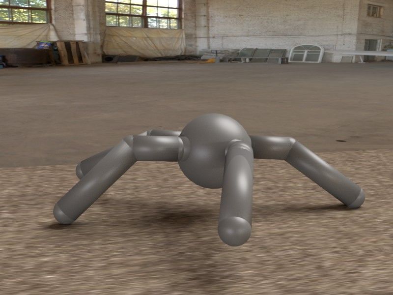
Efficient Differentiable Simulation of Articulated Bodies

  steps        50        100      500    1000    5000                       steps                   50            100                 500           1000           5000
  Ceres       100.0      200.0  1100.0   2700.0 23 600.0                    Ceres                   29.5           29.6                29.5           37.6           62.8
  CppAD        16.0       26.0    160.0    320.0 3100.0                     CppAD                    2.4            2.3                 2.3            2.4            4.8
  JAX         200.0      200.0    400.0    700.0 3000.0                     JAX                    148.1          125.7               127.6          129.6          126.6
  PyTorch    1200.0     2400.0 11 700.0 12 400.0   N/A                      PyTorch                275.7          273.3               280.8          272.1          N/A
  Ours          0.3        0.3      0.7      1.2     5.0                    Ours                     1.2            1.1                 1.2            1.1            1.2

Table 1. Peak memory use of different simulation frameworks.         Table 3. Simulation time for the backward pass. Ours is the
The memory footprint (MB) of our framework is more than two          fastest (in msec). PyTorch crashes at 5,000 simulation steps.
orders of magnitude lower than autodiff methods. PyTorch crashes
at 5,000 simulation steps. ADF fails to compute the gradients in a
reasonable time (10 min) and is not included here for this reason.

  steps        50        100        500      1000       5000
  ADF          25.7       25.5       25.1      32.1       58.4
  Ceres        27.2       27.5       27.2      34.0       58.2
  CppAD         2.4        2.4        2.3       2.3        4.5
  JAX          53.3       46.1       43.1      42.7       42.3
  PyTorch     195.6      192.2      199.2     192.8      N/A                               (a) One Laikago                            (b) Ten Laikago robots
  Ours          0.3        0.3        0.2       0.2        0.2                      30                                                50

                                                                                                                                      40

                                                                      memory (GB)
Table 2. Simulation time for forward pass. Ours is at least an                      20                                                                      CppAD bw

                                                                                                                          time (ms)
                                                                                                                                      30
                                                                                                             CppAD                                          CppAD fw
order of magnitude faster than autodiff tools (in msec). PyTorch                                             Ours                                           Ours bw
                                                                                                                                      20                    Ours fw
crashes at 5,000 simulation steps. CppAD is the fastest baseline.                   10
                                                                                                                                      10

                                                                                     0                                                 0
                                                                                    1000    2000   3000    4000   5000                1000   2000    3000   4000    5000
                                                                                                   steps                                            steps
Eqs. 12 and 14 yield the same gradients with respect to
the action, which provide the gradients of the network pa-                           (c) Memory footprint                                  (d) Time per step
rameters. This method, which we call policy enhancement,             Figure 3. Memory and speed of our method vs. CppAD, the
constructs the loss functions with embedded ground-truth             fastest autodiff method. (a,b) Two scenes used in experiments.
gradients so that the policy updates are physics-aware and           (c,d) Memory consumption and per-step runtime when simulating
generally more accurate than merely looking at the Q func-           ten Laikago robots for different numbers of steps. CppAD crashes
                                                                     when simulating for 5,000 steps due to memory overflow.
tion itself, thus achieving faster convergence and even po-
tentially higher reward.
                                                                     with 32GB of memory.
6. Results
                                                                     One robot. In the first round, we profile all the methods
For experiments, we will first scale the complexity of simu-         by simulating one Laikago robot standing on the ground.
lated scenes and compare the performance of our method               Figure 3(a) provides a visualization. The state vector of the
with autodiff tools. Then we will integrate differentiable           Laikago has 37 dimensions (19-dimensional positions and
physics into reinforcement learning and use our method to            18-dimensional velocities). We vary the number of simula-
learn control policies. Lastly, we will apply differentiable         tion steps from 50 to 5,000. JAX is based on Python and its
articulated dynamics to solve motion control and parameter           JIT compiler cannot easily be used in our C++ simulation
estimation problems.                                                 framework. To test the performance of JAX, we write a sim-
                                                                     ple approximation of our simulator in Python, with similar
6.1. Comparison with Autodiff Tools                                  computational complexity as ours. The simplified test code
                                                                     can be found in the supplement.
Using existing autodiff tools is a convenient way to derive
simulation gradients. However, these tools are not optimized         The memory consumption of different methods is listed
for articulated dynamics, which adversely affects their com-         in Table 1. The memory consumed by autodiff tools is
putation and memory consumption in this domain. We com-              orders of magnitude higher than ours. Among all the auto-
pare our method with state-of-the-art autodiff tools, includ-        differentiation tools, JAX and CppAD are the most memory-
ing CppAD (Bell et al., 2018), Ceres (Agarwal et al., 2010),         efficient. ADF fails to backpropagate the gradients in a
PyTorch (Paszke et al., 2019), autodiff (Leal et al., 2018)          reasonable time. We show in the supplement that the com-
(referred to as ADF to avoid ambiguity), and JAX (Brad-              putation time of backpropagation in ADF is exponential in
bury et al., 2018). All our experiments are performed on a           the depth of the computational graph. Note that articulated
desktop with an Intel(R) Xeon(R) W-2123 CPU @ 3.60GHz                body simulation is intrinsically deep. In this experiment, the
Efficient Differentiable Simulation of Articulated Bodies
depth of one simulation step can reach 103 due to sequen- 1
tial iterative steps in the forward dynamics and the contact 0.8
solver. PyTorch crashes at 5,000 simulation steps because 0.6
Ours
MBPO
ratio
SAC
of memory overflow. 0.4
SQL
PPO
Table 2 reports the average time for a forward simulation 0.2
step. The numbers indicate that our method is faster than 0
2 4 6
others by at least an order of magnitude. Our method has number of links
a constant time complexity per step. The time per step of (a) Pendulum (b) Relative reward
ADF, Ceres, and CppAD increases with the number of steps. 15
20
Note that JAX and Torch are optimized for heavily data- 10
parallel workloads. Articulated body simulation is much 5
Ours
0
Ours
reward
reward
MBPO MBPO
more serial in nature and cannot take full advantage of their 0
SAC
SQL
SAC
SQL
PPO PPO
vectorization. Table 3 reports the time for backward step. -5
-20
Our method is the fastest when computing the gradients.
-10 -40
100 200 300 400 500 200 400 600
Ten robots. To further test the efficiency of our method, episode episode
we simulate a scene with 10 Laikago robots. Figure 3(b) (c) 5-link learning curves (d) 7-link learning curves
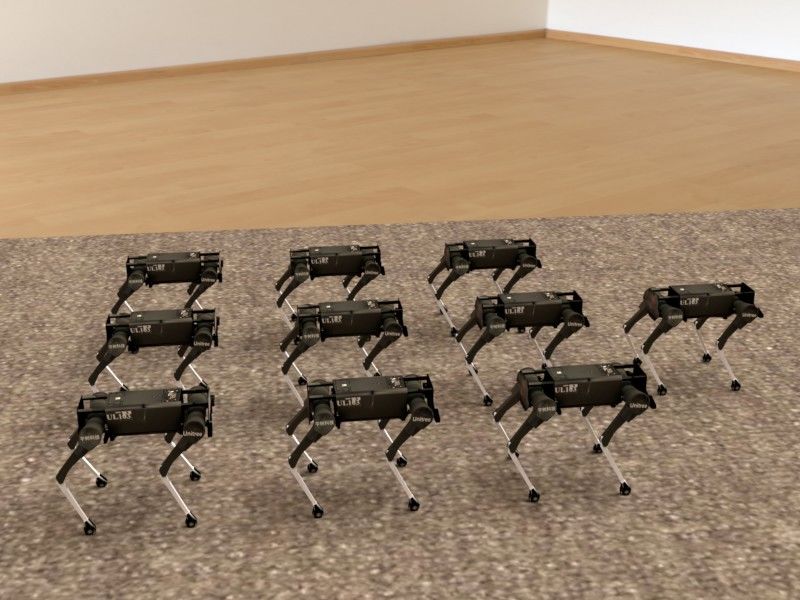
provides a visualization. In this experiment, our method is
Figure 4. The n-link pendulum task. Our method attains higher
compared with CppAD, the best-performing autodiff frame-
reward than MBPO.
work according to the experiments reported in Tables 1
and 2. The number of simulation steps is varied from 1,000
6000
to 5,000. Figure 3(c) shows that the memory footprint of our Ours
MBPO
SAC
method is negligible compared to CppAD. Our method only 4000 SQL
PPO
reward
needs to store 5 KB of data per step, while CppAD needs to
2000
save the full data and topology of the computational graph.
The forward and backward time per step are plotted in Fig- 0
ure 3(d). Our backward pass takes longer than our forward 0 20 40 60 80
episode
pass because the method first runs forward simulation to
reconstruct the intermediate variables. Nevertheless, our (a) Ant walking (b) Reward curve
method is much faster than CppAD and the performance Figure 5. The MuJoCo Ant task. Using our differentiable simu-
gap grows with simulation length. lator to generate extra samples accelerates learning.
6.2. Integration with Reinforcement Learning
target location.
We demonstrate the improvements from the two RL en-
hancement methods described in Section 5. Note that we We trained each model for 100n epochs, where n is the
cannot use the two methods together because policy en- number of links. The results are shown in Figure 4. In Fig-
hancement requires the gradients at the sample point, which ure 4(b), we report the relative reward of each task, which is
the extra samples from sample enhancement do not have defined as the attained reward divided by the maximal possi-
(unless higher-order gradients are computed). Thus, we ble reward. MBPO works well in easy scenarios with up to
test the two techniques separately. We use the model-based 3 links, but its performance degrades starting at 4 links. In
MBPO optimizer as the main baseline (Janner et al., 2019). contrast, our model reaches close to the best possible reward
All networks use the PyTorch default initialization scheme. for all systems. The learning curves for the 5-link and 7-link
systems are shown in Figure 4(c,d). MBPO does not attain
N-link pendulum. We first test our policy enhancement satisfactory results for 6- and 7-link systems. We observed
method in a simple scenario, where an n-link pendulum that around the 100th epoch, the losses for the Q function of
needs to reach a target point by applying torques on each the MBPO method increased a lot. We hypothesize that this
of the joints under gravity (Figure 4(a)). The target point is because the complexity of the physical system exceeds
is fixed to be the highest point reachable, and initially the the expressive power of the model network in MBPO.
pendulum is positioned horizontally. The reward function is
the progress to the target between consecutive steps: MuJoCo Ant. Next, we test our sample enhancement
method on the MuJoCo Ant. In this scenario, a four-legged
r = kxt − xg k2 − kxt−1 − xg k2 , (15) robot on the ground needs to learn to walk towards a fixed
heading (Figure 5(a)). The scenario is the same as the stan-
where xt is the end-effector location at time t, and xg is the dard task defined in MuJoCo, except that the simulator isEfficient Differentiable Simulation of Articulated Bodies
0.1
CMA-ES
0.08
objective function
Ours
0.06
0.04
0.02
0
0 20 40
episode
0.25 0.8
(a) A racecar (b) Loss per episode
CMA-ES CMA-ES
0.2 0.1 1
objective function
Ours objective function 0.6 Ours CMA-ES loss
0.08 0.8
objective function
0.15 Ours ground truth
loss function
0.4
0.1 0.06 0.6
0.2 0.04 0.4
0.05
0.02 0.2
0 0
0 200 400 0 500 1000 1500
0 0
episode episode 0 5 10 15 0 0.5 1 1.5
time (s) frictional coefficient
0.25 0.8
CMA-ES CMA-ES (c) Loss over time (d) Loss landscape
0.2
objective function
objective function
Ours 0.6 Ours
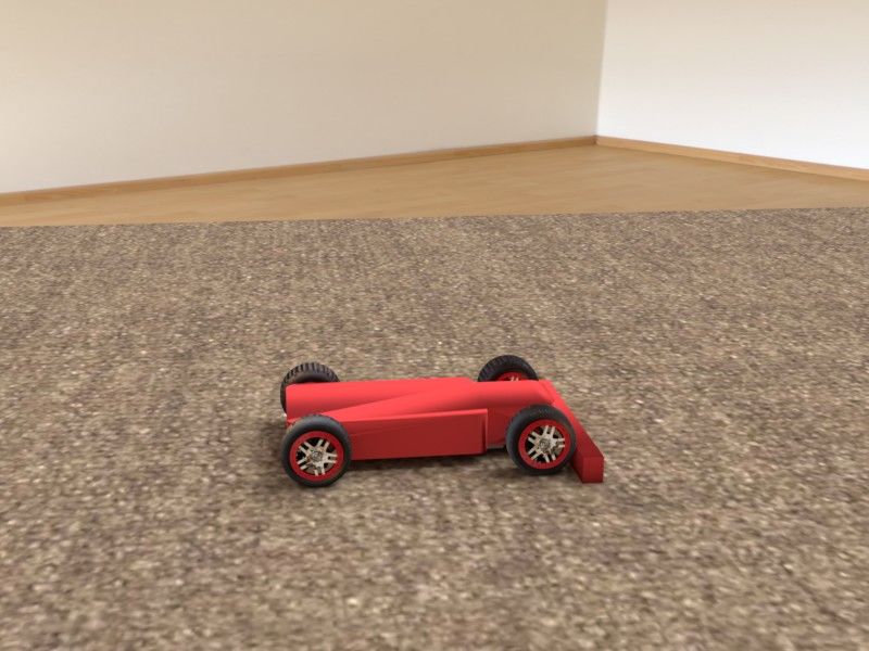
0.15 Figure 7. Parameter estimation. The goal is to estimate the slid-
0.4
0.1 ing friction coefficient that makes the racecar decelerate to a target
0.05
0.2 location. (b,c) Loss curves in episode and wall-clock time, respec-
0 0
tively. (d) Loss landscape plot. SGD with gradients computed by
0 50 100 0 20 40 60 our method solves the task within 10 iterations, more accurately
time (s) time (s)
and faster than the gradient-free baseline.
(a) Throwing (b) Hitting
Figure 6. Motion control. The task is to optimize the torque vec-
using a 9-DoF robot arm and (b) hitting a golf ball to a target
tors to (a) throw a ball with an articulated 9-DoF robot arm and
(b) hit a golf ball with an articulated linkage. In both scenarios, location using an articulated linkage. These tasks are also
the goal is for the ball to settle at a specified target location. SGD shown in the supplementary video.
with gradients provided by our method converges within 20 and 50 For both scenarios, a torque vector is applied to the joints
steps, respectively, while gradient-free optimization fails to reach
in each time step. Assume there are n time steps and k
comparable accuracy even with more than an order of magnitude
DoFs. The torque variable to be optimized has n × k di-
higher number of iterations. The third row indicates that even
though CMA-ES does not compute gradients, our method is still mensions, and the objective function is the L2 distance from
faster overall in wall-clock time. the ball’s actual position to the target. The joint positions
and the torques are initialized as 0. If no gradients are
available, a derivative-free optimization algorithm such as
replaced by ours. We also compare with other methods CMA-ES (Hansen, 2016) can be used. We plot the loss
(SAC (Haarnoja et al., 2018), SQL (Haarnoja et al., 2017), curves of our method and CMA-ES in Figure 6.
and PPO (Schulman et al., 2017) implemented in Ray RL-
lib (Liang et al., 2018)) for reference. For every true sample In (a), SGD with gradients from our simulator converges
we get from the simulator, we generate 9 extra samples in 20 steps. In contrast, CMA-ES does not reach the same
around it using our sample enhancement method. Other accuracy even after 500 steps. In (b), SGD with gradients
than that, everything is the same as in MBPO. We repeat from our simulator converges in 50 steps, while CMA-ES
the training 4 times for all methods. Figure 5(b) shows the does not reach the same accuracy even after 1500 steps.
reward over time. Our method exhibits faster convergence. Parameter estimation. Our method can estimate unknown
We can also transfer the policy trained in our differentiable physical parameters from observation. In Figure 7, a racecar
simulator to MuJoCo. This tests the fidelity of our simulator starts with horizontal velocity 1m/s. The wheels and the
and robustness of the learned policy to simulator details. steering system are articulated. We estimate the sliding fric-
The results are reported in the supplement. tion coefficient µ between the wheels and the ground such
that the car stops at x = 0.8m at the end of the episode. At
6.3. Applications the initial guess µ = 0.002, the car reaches x = 1.0m. We
use gradient descent to optimize the estimated friction coef-
Motion control. Differentiable physics enables application ficient. After 10 iterations of SGD with gradients provided
of gradient-based optimization to learning and control prob- by our method, the car reaches the goal with µ = 0.21. In
lems that involve physical systems. In Figure 6, we show comparison, the gradient-free baseline takes multiple times
two physical tasks: (a) throwing a ball to a target location longer to reach comparable objective values.Efficient Differentiable Simulation of Articulated Bodies
7. Conclusion Bogatskiy, A., Anderson, B. M., Offermann, J. T., Roussi,
M., Miller, D. W., and Kondor, R. Lorentz group equivari-
We have developed a differentiable simulator for articulated ant neural network for particle physics. In ICML, 2020.
body dynamics that runs 10x faster with 100x smaller mem-
ory footprint in comparison to existing autodiff tools. To Bradbury, J., Frostig, R., Hawkins, P., Johnson, M. J., Leary,
achieve this performance gain, we analyze the workload C., Maclaurin, D., Necula, G., Paszke, A., VanderPlas, J.,
of each simulation step to better manage computation and Wanderman-Milne, S., and Zhang, Q. JAX: Composable
memory. The adjoint method is used to compute the gra- transformations of Python+NumPy programs. http:
dients of the simulation. We derive the adjoints of spatial //github.com/google/jax, 2018.
algebra and the Gauss-Seidel solver. We then adapt the
checkpointing method to deal with the sequential nature of Chang, M. B., Ullman, T., Torralba, A., and Tenenbaum,
articulated body simulation, reducing memory consumption J. B. A compositional object-based approach to learning
by two orders of magnitude. physical dynamics. In ICLR, 2017.
As a supporting contribution, we have explored two applica- Chen, R. T. Q., Rubanova, Y., Bettencourt, J., and Duvenaud,
tions of differentiable physics to reinforcement learning with D. K. Neural ordinary differential equations. In Neural
physical systems, reporting preliminary results that indicate Information Processing Systems, 2018.
that differentiable physics can accelerate learning. We have
Chen, T., Xu, B., Zhang, C., and Guestrin, C. Training deep
also presented application scenarios that clearly demonstrate
nets with sublinear memory cost. arXiv:1604.06174,
the effectiveness of gradient-based optimization in motion
2016.
control and parameter estimation with articulated physical
systems. Chen, Z., Zhang, J., Arjovsky, M., and Bottou, L. Symplec-
tic recurrent neural networks. In ICLR, 2020.
Acknowledgements. This research is supported in part by
Intel Corporation, National Science Foundation, Dr. Barry Coumans, E. Bullet physics simulation. In ACM SIG-
Mersky and Capital One Endowed Professorship, and Eliza- GRAPH Courses, 2015.
beth Stevinson Iribe Endowed Chair Professorship.
Coumans, E. et al. Tiny differentiable simula-
tor. https://github.com/google-research/
References tiny-differentiable-simulator, 2020.
Abadi, M., Barham, P., Chen, J., Chen, Z., Davis, A., Dean,
J., Devin, M., Ghemawat, S., Irving, G., Isard, M., et al. Cranmer, M., Greydanus, S., Hoyer, S., Battaglia, P.,
TensorFlow: A system for large-scale machine learning. Spergel, D., and Ho, S. Lagrangian neural networks.
In OSDI, 2016. In ICLR Workshops, 2020.
Agarwal, S., Mierle, K., et al. Ceres solver. http:// de Avila Belbute-Peres, F., Smith, K. A., Allen, K. R., Tenen-
ceres-solver.org, 2010. baum, J., and Kolter, J. Z. End-to-end differentiable
physics for learning and control. In Neural Information
Anderson, B. M., Hy, T., and Kondor, R. Cormorant: Co- Processing Systems, 2018.
variant molecular neural networks. In Neural Information
Processing Systems, 2019. Degrave, J., Hermans, M., Dambre, J., and wyffels, F. A
differentiable physics engine for deep learning in robotics.
Battaglia, P. W., Pascanu, R., Lai, M., Rezende, D., and Frontiers in Neurorobotics, 13, 2019.
Kavukcuoglu, K. Interaction networks for learning about
objects, relations and physics. In Neural Information Du, T., Wu, K., Spielberg, A., Matusik, W., Zhu, B., and
Processing Systems, 2016. Sifakis, E. Functional optimization of fluidic devices with
differentiable stokes flow. ACM Trans. Graph., 2020.
Belbute-Peres, F. d. A., Economon, T. D., and Kolter, J. Z.
Combining differentiable PDE solvers and graph neural Featherstone, R. Rigid body dynamics algorithms. 2007.
networks for fluid flow prediction. In ICML, 2020.
Featherstone, R. Spatial vector and dynamics software.
Bell, B. M. et al. CppAD: C++ algorithmic differ- http://royfeatherstone.org/spatial/,
entiation. https://projects.coin-or.org/ 2008.
CppAD, 2018.
Geilinger, M., Hahn, D., Zehnder, J., Bächer, M.,
Bern, J. M., Banzet, P., Poranne, R., and Coros, S. Trajectory Thomaszewski, B., and Coros, S. ADD: Analytically
optimization for cable-driven soft robot locomotion. In differentiable dynamics for multi-body systems with fric-
Robotics: Science and Systems (RSS), 2019. tional contact. ACM Trans. Graph., 39(6), 2020.Efficient Differentiable Simulation of Articulated Bodies
Giles, M. B. and Pierce, N. A. An introduction to the adjoint Janner, M., Fu, J., Zhang, M., and Levine, S. When to trust
approach to design. Flow, Turbulence and Combustion, your model: Model-based policy optimization. In Neural
65(3-4):393–415, 2000. Information Processing Systems, 2019.
Griewank, A. and Walther, A. Revolve: An implementation Kirisame, M., Lyubomirsky, S., Haan, A., Brennan, J., He,
of checkpointing for the reverse or adjoint mode of com- M., Roesch, J., Chen, T., and Tatlock, Z. Dynamic tensor
putational differentiation. ACM Trans. Math. Softw., 26 rematerialization. In ICLR, 2021.
(1):19–45, 2000.
Krishna Murthy, J., Iyer, G., and Paull, L. gradSLAM:
Griewank, A. and Walther, A. Evaluating Derivatives: Dense SLAM meets automatic differentiation. In ICRA,
Principles and Techniques of Algorithmic Differentiation. 2020.
SIAM, 2008.
Krishna Murthy, J., Macklin, M., Golemo, F., Voleti, V.,
Gruslys, A., Munos, R., Danihelka, I., Lanctot, M., and Petrini, L., Weiss, M., Considine, B., Parent-Lévesque, J.,
Graves, A. Memory-efficient backpropagation through Xie, K., Erleben, K., et al. gradSim: Differentiable sim-
time. In Neural Information Processing Systems, 2016. ulation for system identification and visuomotor control.
In ICLR, 2021.
Haarnoja, T., Tang, H., Abbeel, P., and Levine, S. Rein-
forcement learning with deep energy-based policies. In Laine, S., Hellsten, J., Karras, T., Seol, Y., Lehtinen, J., and
ICML, 2017. Aila, T. Modular primitives for high-performance differ-
entiable rendering. ACM Trans. Graph., 39(6), 2020.
Haarnoja, T., Zhou, A., Abbeel, P., and Levine, S. Soft actor-
critic: Off-policy maximum entropy deep reinforcement Leal, A. et al. autodiff: automatic differentiation made eas-
learning with a stochastic actor. In ICML, 2018. ier for C++. https://github.com/autodiff/
autodiff, 2018.
Hansen, N. The CMA evolution strategy: A tutorial.
arXiv:1604.00772, 2016. Lee, J., Grey, M., Ha, S., Kunz, T., Jain, S., Ye, Y., Srinivasa,
Heiden, E., Millard, D., Zhang, H., and Sukhatme, G. S. S., Stilman, M., and Liu, C. DART: Dynamic animation
Interactive differentiable simulation. arXiv:1905.10706, and robotics toolkit. The Journal of Open Source Soft-
2019. ware, 3, 2018.
Heiden, E., Millard, D., Coumans, E., Sheng, Y., and Li, T.-M., Aittala, M., Durand, F., and Lehtinen, J. Differ-
Sukhatme, G. S. NeuralSim: Augmenting differentiable entiable monte carlo ray tracing through edge sampling.
simulators with neural networks. arXiv:2011.04217, ACM Trans. Graph., 37(6), 2018a.
2020.
Li, T.-M., Gharbi, M., Adams, A., Durand, F., and Ragan-
Holl, P., Koltun, V., and Thuerey, N. Learning to control Kelley, J. Differentiable programming for image process-
PDEs with differentiable physics. In ICLR, 2020. ing and deep learning in Halide. ACM Trans. Graph., 37
(4), 2018b.
Hu, Y., Liu, J., Spielberg, A., Tenenbaum, J. B., Free-
man, W. T., Wu, J., Rus, D., and Matusik, W. Chain- Li, T.-M., Lukáč, M., Michaël, G., and Ragan-Kelley, J.
Queen: A real-time differentiable physical simulator for Differentiable vector graphics rasterization for editing
soft robotics. In ICRA, 2019. and learning. ACM Trans. Graph., 39(6), 2020.
Hu, Y., Anderson, L., Li, T.-M., Sun, Q., Carr, N., Ragan- Li, Y., Wu, J., Zhu, J.-Y., Tenenbaum, J. B., Torralba, A.,
Kelley, J., and Durand, F. DiffTaichi: Differentiable and Tedrake, R. Propagation networks for model-based
programming for physical simulation. In ICLR, 2020. control under partial observation. In ICRA, 2019.
Huang, Z., Hu, Y., Du, T., Zhou, S., Su, H., Tenenbaum, Liang, E., Liaw, R., Nishihara, R., Moritz, P., Fox, R., Gold-
J. B., and Gan, C. PlasticineLab: A soft-body manipu- berg, K., Gonzalez, J. E., Jordan, M. I., and Stoica, I.
lation benchmark with differentiable physics. In ICLR, RLlib: Abstractions for distributed reinforcement learn-
2021. ing. In ICML, 2018.
Ingraham, J., Riesselman, A., Sander, C., and Marks, D. Liang, J., Lin, M. C., and Koltun, V. Differentiable cloth
Learning protein structure with a differentiable simulator. simulation for inverse problems. In Neural Information
In ICLR, 2019. Processing Systems, 2019.Efficient Differentiable Simulation of Articulated Bodies
McNamara, A., Treuille, A., Popovic, Z., and Stam, J. Fluid Shah, A., Wu, C.-Y., Mohan, J., Chidambaram, V., and
control using the adjoint method. ACM Trans. Graph., 23 Krähenbühl, P. Memory optimization for deep networks.
(3), 2004. In ICLR, 2021.
Mrowca, D., Zhuang, C., Wang, E., Haber, N., Li, F., Tenen- Song, C. and Boularias, A. Learning to slide unknown ob-
baum, J., and Yamins, D. L. Flexible neural representa- jects with differentiable physics simulations. In Robotics:
tion for physics prediction. In Neural Information Pro- Science and Systems (RSS), 2020a.
cessing Systems, 2018.
Song, C. and Boularias, A. Identifying mechanical models
Nimier-David, M., Vicini, D., Zeltner, T., and Jakob, W. of unknown objects with differentiable physics simula-
Mitsuba 2: A retargetable forward and inverse renderer. tions. In L4DC, 2020b.
ACM Trans. Graph., 38(6), 2019.
Spielberg, A., Zhao, A., Hu, Y., Du, T., Matusik, W., and
Nimier-David, M., Speierer, S., Ruiz, B., and Jakob, W. Ra- Rus, D. Learning-in-the-loop optimization: End-to-end
diative backpropagation: An adjoint method for lightning- control and co-design of soft robots through learned deep
fast differentiable rendering. ACM Trans. Graph., 39(4), latent representations. In Neural Information Processing
2020. Systems, 2019.
Paszke, A., Gross, S., Massa, F., Lerer, A., Bradbury, J., Stepien, J. Physics-Based Animation of Articulated Rigid
Chanan, G., Killeen, T., Lin, Z., Gimelshein, N., Antiga, Body Systems for Virtual Environments. PhD thesis, 2013.
L., et al. PyTorch: An imperative style, high-performance
deep learning library. In Neural Information Processing Takahashi, T., Liang, J., Qiao, Y.-L., and Lin, M. C. Dif-
Systems, 2019. ferentiable fluids with solid coupling for learning and
control. In AAAI, 2021.
Pfaff, T., Fortunato, M., Sanchez-Gonzalez, A., and
Battaglia, P. Learning mesh-based simulation with graph Tedrake, R. et al. Drake: Model-based design and verifica-
networks. In ICLR, 2021. tion for robotics. https://drake.mit.edu, 2019.
Qiao, Y.-L., Liang, J., Koltun, V., and Lin, M. C. Scalable Todorov, E., Erez, T., and Tassa, Y. MuJoCo: A physics
differentiable physics for learning and control. In ICML, engine for model-based control. In IROS, 2012.
2020.
Toussaint, M., Allen, K., Smith, K., and Tenenbaum, J.
Sanchez-Gonzalez, A., Heess, N., Springenberg, J. T., Differentiable physics and stable modes for tool-use and
Merel, J., Riedmiller, M., Hadsell, R., and Battaglia, P. manipulation planning. In Robotics: Science and Systems
Graph networks as learnable physics engines for infer- (RSS), 2018.
ence and control. In ICML, 2018.
Ummenhofer, B., Prantl, L., Thürey, N., and Koltun, V.
Sanchez-Gonzalez, A., Godwin, J., Pfaff, T., Ying, R., Lagrangian fluid simulation with continuous convolutions.
Leskovec, J., and Battaglia, P. W. Learning to simulate In ICLR, 2020.
complex physics with graph networks. In ICML, 2020.
Wandel, N., Weinmann, M., and Klein, R. Learning in-
Schenck, C. and Fox, D. SPNets: Differentiable fluid dy- compressible fluid dynamics from scratch – towards fast,
namics for deep neural networks. In Conference on Robot differentiable fluid models that generalize. In ICLR, 2021.
Learning (CoRL), 2018.
Wang, K., Aanjaneya, M., and Bekris, K. E. A first princi-
Schoenholz, S. S. and Cubuk, E. D. JAX M.D.: End-to-end ples approach for data-efficient system identification of
differentiable, hardware accelerated, molecular dynam- spring-rod systems via differentiable physics engines. In
ics in pure Python. In Neural Information Processing L4DC, 2020.
Systems, 2020.
Zhuang, J., Dvornek, N. C., Li, X., Tatikonda, S., Pa-
Schulman, J., Wolski, F., Dhariwal, P., Radford, A., and pademetris, X., and Duncan, J. S. Adaptive checkpoint
Klimov, O. Proximal policy optimization algorithms. adjoint method for gradient estimation in neural ODE. In
arXiv:1707.06347, 2017. ICML, 2020.
Schütt, K., Kindermans, P., Felix, H. E. S., Chmiela, S.,
Tkatchenko, A., and Müller, K. SchNet: A continuous-
filter convolutional neural network for modeling quantum
interactions. In Neural Information Processing Systems,
2017.You can also read