Reflected fractional Brownian motion in one and higher dimensions - Ralf Metzler
←
→
Page content transcription
If your browser does not render page correctly, please read the page content below
PHYSICAL REVIEW E 102, 032108 (2020)

                         Reflected fractional Brownian motion in one and higher dimensions

  Thomas Vojta ,1 Samuel Halladay ,1 Sarah Skinner,1 Skirmantas Janušonis ,2 Tobias Guggenberger,3 and Ralf Metzler3
                     1
                      Department of Physics, Missouri University of Science and Technology, Rolla, Missouri 65409, USA
    2
        Department of Psychological and Brain Sciences, University of California, Santa Barbara, Santa Barbara, California 93106, USA
                        3
                          Institute of Physics and Astronomy, University of Potsdam, D-14476 Potsdam-Golm, Germany

                                    (Received 8 May 2020; accepted 24 July 2020; published 8 September 2020)

                   Fractional Brownian motion (FBM), a non-Markovian self-similar Gaussian stochastic process with long-
                ranged correlations, represents a widely applied, paradigmatic mathematical model of anomalous diffusion. We
                report the results of large-scale computer simulations of FBM in one, two, and three dimensions in the presence
                of reflecting boundaries that confine the motion to finite regions in space. Generalizing earlier results for finite
                and semi-infinite one-dimensional intervals, we observe that the interplay between the long-time correlations
                of FBM and the reflecting boundaries leads to striking deviations of the stationary probability density from
                the uniform density found for normal diffusion. Particles accumulate at the boundaries for superdiffusive FBM
                while their density is depleted at the boundaries for subdiffusion. Specifically, the probability density P develops
                a power-law singularity, P ∼ r κ , as a function of the distance r from the wall. We determine the exponent κ as a
                function of the dimensionality, the confining geometry, and the anomalous diffusion exponent α of the FBM. We
                also discuss implications of our results, including an application to modeling serotonergic fiber density patterns
                in vertebrate brains.

                DOI: 10.1103/PhysRevE.102.032108

                         I. INTRODUCTION                                    matical model of a stochastic process with long-time cor-
                                                                            related steps is fractional Brownian motion (FBM) which
   Following pioneering works of Einstein [1], Smoluchowski
                                                                            was introduced by Kolmogorov [11] and further studied by
[2], and Langevin [3], normal diffusion can be understood as
                                                                            Mandelbrot and van Ness [12]. FBM is a self-similar Gaus-
random motion that is local in time and space. This means
                                                                            sian stochastic process with stationary long-time correlated
that normal diffusion is a stochastic process that fulfills two
                                                                            increments. It gives rise to power-law anomalous diffusion
conditions, (i) it features a finite correlation time after which
                                                                            (1). In the superdiffusive regime, 1 < α < 2, the motion is
individual steps become statistically independent, and (ii) the
                                                                            persistent (positive correlations between the steps) whereas
displacements over a correlation time feature a finite second
                                                                            it is antipersistent (negative correlations) in the subdiffu-
moment. If these conditions are fulfilled, the central limit
                                                                            sive regime, 0 < α < 1. In the marginal case α = 1, FBM
theorem applies, resulting in the well-known linear relation
                                                                            is identical to normal Brownian motion with uncorrelated
r2  ∼ t between the mean-square displacement of the mov-
                                                                            steps.
ing particle and the elapsed time t [4].
                                                                                FBM has been applied to model the dynamics in a wide
   If at least one of the preconditions for the central limit
                                                                            variety of systems, including diffusion inside biological cells
theorem is violated, deviations from the linear relation r2  ∼
                                                                            [13–18], the dynamics of polymers [19,20], electronic net-
t may appear, giving rise to anomalous diffusion (for reviews
                                                                            work traffic [21], as well as fluctuations of financial markets
see, e.g., Refs. [5–10] and references therein). For example,
                                                                            [22,23]. FBM has been analyzed quite extensively in the
sufficiently broad distributions of waiting times between in-
                                                                            mathematical literature (see, e.g., Refs. [24–27]) but only
dividual steps can lead to subdiffusive motion (for which
                                                                            few results are available for FBM in confined geometries,
r2  increases slower than t) while broad distributions of step
                                                                            i.e., in the presence of nontrivial boundary conditions. These
sizes may produce superdiffusion (where r2  increases faster
                                                                            include the solution of the first-passage problem of FBM
than t). Anomalous diffusion is often characterized by the
                                                                            confined to a semi-infinite interval [28–31]), a conjecture for
power-law dependence
                                                                            a two-dimensional wedge domain [32], and corresponding
                             r2  ∼ t α ,                          (1)     results for parabolic domains [33]. In addition, the probability
                                                                            density of FBM on a semi-infinite interval with an absorbing
where α is the anomalous diffusion exponent which takes                     boundary was investigated in Refs. [34–36]. The difficulties
values 1 < α < 2 for superdiffusion and 0 < α < 1 for                       in analyzing FBM in confined geometries are related to the
subdiffusion.                                                               fact that a generalized diffusion equation for FBM applicable
   Another important mechanism leading to anomalous dif-                    to solve boundary-value problems is yet to be found, and
fusion consists of long-range correlations in time between                  the method of images [5,37], typically invoked for boundary-
the displacements of the particle. The prototypical mathe-                  value problems, fails.

2470-0045/2020/102(3)/032108(13)                                     032108-1                                  ©2020 American Physical Society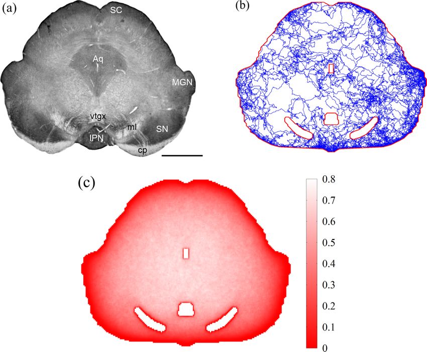
THOMAS VOJTA et al.                                                                        PHYSICAL REVIEW E 102, 032108 (2020)

    Recently, FBM with reflecting walls has attracted consid-      the Gaussian form
erable attention as computer simulations have demonstrated
                                                                                                  1             x2
that the interplay between the long-time correlations and the                    P(x, t ) = √         exp −          .         (3)
                                                                                              4π Kt α         4Kt α
confinement modifies the probability density function P(x, t )
of the diffusing particles. For FBM on a semi-infinite interval    We now discretize time by defining xn = X (tn ) with tn = n
with a reflecting wall at the origin, the probability density      where  is the time step and n is an integer. This leads to
becomes highly non-Gaussian and develops a power-law sin-          a discrete version of FBM [43] that lends itself to computer
gularity, P ∼ x κ , at the wall [38,39]. For persistent noise      simulations. It can be understood as a random walk with iden-
(superdiffusive FBM), particles accumulate at the wall, κ < 0,     tically Gaussian distributed but long-time correlated steps.
whereas particles are depleted near the wall, κ > 0 for antiper-   Specifically, the position xn of the particle evolves according
sistent noise (subdiffusive FBM). Analogous simulations of         to the recursion relation
FBM on a finite interval, with reflecting walls at both ends,                                xn+1 = xn + ξn .                      (4)
have shown that the stationary probability density deviates
from the uniform distribution found for normal diffusion [40].     The increments ξn are a discrete fractional Gaussian noise,
Particles accumulate at the walls and are depleted in the          a stationary Gaussian process of zero mean, variance σ 2 =
middle of the interval for persistent noise whereas the opposite   2K α , and covariance function
is true for antipersistent noise.
                                                                        Cn = ξm ξm+n  = 21 σ 2 (|n + 1|α − 2|n|α + |n − 1|α ).   (5)
    The above results for the probability density of reflected
FBM are all restricted to one dimension whereas many of            The correlations are positive (persistent) for α > 1 and neg-
the applications in physics, biology and beyond are in two or      ative (antipersistent) for α < 1. In the marginal case, α =
three dimensions. It is therefore interesting and important to     1, the covariance vanishes for all n = 0, i.e., we recover
ask whether reflected FBM in higher dimensions also features       normal Brownian motion. For n → ∞, the covariance takes
unusual accumulation and depletion effects of particles near       the power-law form ξm ξm+n  ∼ α(α − 1)|n|α−2 .
reflecting boundaries and to determine the functional form of         To reach the continuum limit, the time step  needs to be
the probability density in these cases.                            small compared with the considered times t. Equivalently, the
    In the present paper, we therefore analyze by means of         size σ of an individual increment must be small compared
large-scale computer simulations the properties of reflected       with the considered distances or system sizes. This can be
FBM in various confined geometries. After providing some           achieved either by taking  to zero at fixed t or, equivalently,
additional results in one dimension, the main focus will be        by taking t to infinity at fixed . In this paper, we chose
on reflected FBM in two and three space dimensions. In all         the latter route by fixing  = const. and considering times
cases, we find that particles accumulate at the reflecting walls   t → ∞.
for persistent noise and are depleted close to the walls for          We now generalize FBM from one to higher dimensions.
antipersistent noise, just as in one dimension. The probability    FBM in d dimensions can be defined as the superposition
density behaves as a power of the distance from the wall,          of d independent FBM processes, one for each Cartesian
P ∼ r κ . We determine the exponent κ as a function of the         coordinate [44,45]. This means the d-dimensional position
dimensionality, the confining geometry, and the anomalous          vector rn follows the recursion relation
diffusion exponent α of the FBM.
                                                                                             rn+1 = rn + ξ n ,                     (6)
    Our paper is organized as follows: We define reflected
FBM in one and higher dimensions in Sec. II, where we also         where the components        ξn(i)
                                                                                                of the d-dimensional fractional
discuss the details of our numerical approach. Sections III,       Gaussian noise feature the covariance function
IV, and V are devoted to results for one, two, and three space           (i) ( j)  1 2
                                                                         ξm ξm+n = 2 σ (|n + 1|α − 2|n|α + |n − 1|α )δi j . (7)
dimensions, respectively. In Sec. VI, we discuss an interesting
application of reflected FBM to model serotonergic fibers in       It is easy to show that this definition is invariant under
vertebrate brains [41,42]. We conclude in Sec. VII.                rotations of the coordinate system. We also note that the
                                                                   generalization of FBM to higher dimensions as superposition
                                                                   of independent components is not unique. More complicated
  II. REFLECTED FRACTIONAL BROWNIAN MOTION
                                                                   correlation structures between the components have been
         A. Definition of fractional Brownian motion               considered in the mathematical literature (see, e.g., Ref. [46]).
   We start by defining FBM in one space dimension. FBM
is a continuous-time centered Gaussian stochastic process.                              B. Reflecting boundaries
The covariance function of the position X at times s and t is         Let us now discuss how to define the boundary conditions
given by                                                           that confine the FBM to a given geometry. Reflecting walls
                                                                   can be implemented by suitably modifying the recursion
            X (s)X (t ) = K (sα − |s − t|α + t α ),       (2)    relations (4) and (6). As the fractional Gaussian noise is
                                                                   understood as externally given [47], it is not affected by the
defined for anomalous diffusion exponents α in the range
                                                                   walls. In one dimension, an “elastic” wall at position w that
0 < α < 2. Setting s = t, this yields anomalous diffusion with
                                                                   restricts the motion to x  w (i.e., a wall to the left of the
a mean-square displacement of X 2  = 2Kt α , i.e., superdiffu-
                                                                   allowed interval) can be defined by means of
sion for α > 1 and subdiffusion for α < 1. Correspondingly,
the probability density of unconfined (free space) FBM takes                           xn+1 = w + |xn + ξn − w|.                   (8)

                                                             032108-2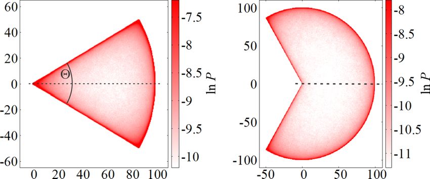
REFLECTED FRACTIONAL BROWNIAN MOTION IN ONE …                                                PHYSICAL REVIEW E 102, 032108 (2020)

This definition was employed in recent studies of reflected            between 0.3 (deep in the subdiffusive regime) and 1.95 (deep
FBM [38–40,45], but it is by no means unique. The recursion            in the superdiffusive regime and almost at the ballistic limit
relation                                                               α = 2). Each simulation uses a large number of particles,
                                                                      up to 107 . We fix the time step at  = 1 and set K = 1/2
                     x + ξn if xn + ξn  w
             xn+1 = n                                   (9)            (unless noted otherwise). This implies a variance σ 2 = 1 of
                     xn        otherwise
                                                                       the individual steps. Each particle performs up to 229 ≈ 5.4 ×
defines an “inelastic” wall at which the particle does not move        108 time steps.
at all if the step would take it into the forbidden region x < w.          As discussed in Sec. II A, this large number of steps
Alternatively, the recursion                                           allows us to reach the continuum (scaling) limit for which
                                                                       the time discretization becomes unimportant, and the behavior
                    xn+1 = max (xn + ξn , w)                   (10)
                                                                       approaches that of continuous time FBM. Expressed in terms
places the particle right at the wall if the step would take it into   of the linear system size L, the continuum limit takes the form
the forbidden region x < w. Definition (10) can be understood          L/σ      1. In our simulations, the linear system sizes range
as a discretized version of the definition of reflected FBM            from L = 100 for the most subdiffusive α = 0.3 to L = 106
in the mathematical literature where it is employed, e.g., in          for some calculations using α values close to two.
queueing theory [48,49].                                                   The correlated Gaussian random numbers ξn that repre-
   In addition to these hard walls one can also introduce soft         sent the fractional noise are precalculated before each actual
walls by adding repulsive forces to the recursion relation,            simulation by means of the Fourier-filtering technique [50].
                                                                       For each Cartesian component of the noise, this method starts
                    xn+1 = xn + ξn + F (xn ).                  (11)    from a sequence of independent Gaussian random numbers
We consider exponential forces,                                        χi of zero mean and unit variance (which we generate by
                                                                       using the Box-Muller transformation with the LFSR113 ran-
                  F (x) = F0 exp [−λ(x − w)],                  (12)    dom number generator proposed by L’Ecuyer [51] as well
characterized by amplitude F0 and decay constant λ. Note that          as the 2005 version of Marsaglia’s KISS [52]). The Fourier
a factor  stemming from the time step has been absorbed               transform χ̃ω of these numbers is then converted via ξ̃ω =
in the amplitude F0 . Boundaries restricting the motion to             [C̃(ω)]1/2 χ̃ω , where C̃(ω) is the Fourier transform of the
positions x  w (i.e., walls at the right end of an allowed            covariance function (5). The inverse Fourier transformation
interval) can be defined in analogy to Eqs. (8) to (11).               of ξ̃ω gives the desired noise values.
   In higher dimensions, we use appropriate generalizations
of the wall implementations (8), (9), and (11). This is unam-                          III. ONE SPACE DIMENSION
biguous for the “inelastic” wall which prevents the particle
                                                                                        A. Summary of earlier results
from moving if it would enter the forbidden region,
                                                                          Wada et al. [38,39] recently employed computer simula-
              r + ξ n if rn + ξ n is in allowed region                 tions to study one-dimensional FBM restricted to the semi-
    rn+1 = n                                              (13)
              rn        otherwise.                                     infinite interval (0, ∞) by a reflecting wall at the origin.
For other wall implementations, some care is required to               They observed that the mean-square displacement x 2  of a
properly deal with the directions of the motion and of the wall        particle that starts at the origin follows the expected power
forces, in particular in complex geometries. For example, a            law t α just as for unconfined FBM. However, the probability
simple reflection analogous to Eq. (8) becomes ambiguous               density was found to be highly non-Gaussian with particles
if the allowed region features sharp corners, and, unless the          accumulating at the wall in the superdiffusive regime α > 1.
geometry is highly symmetric, the directions of the wall forces        For subdiffusive FBM, α < 1, particles are depleted near the
depend on details of the modeling potential.                           wall.
    In the following, the majority of our simulations utilize the          More specifically, the probability density function P(x, t )
“inelastic” walls (9) and (13). However, for reflected FBM to          of the particle position x at time t fulfills the scaling form
be a well-defined self-contained concept, it is important to es-                                    1
tablish that its properties do not depend on the precise choice                        P(x, t ) =        Zα [x/(σ t α/2 )]         (14)
                                                                                                 σ t α/2
of boundary conditions (so that it can be applied to situations
in which details of the interactions between the particles and         in the continuum limit x        σ . The dimensionless scaling
the wall are not known). In Sec. III C, we therefore carefully         function Zα (z) is non-Gaussian near the wall; it develops a sin-
compare trajectories and probability densities resulting from          gularity for z → 0. Based on the extensive simulation results,
different wall implementations. The data show that the wall            Wada et al. conjectured a power-law singularity Zα (z) ∼ zκ
implementations affect the immediate vicinity of the wall only         for z    1 with the exponent given by κ = 2/α − 2.
and become unimportant in the continuum limit, i.e., on length            Analogous results were also obtained for biased FBM on
scales large compared with σ and λ−1 .                                 the interval (0, ∞) [39]. If the bias is towards the wall, a
                                                                       stationary distribution develops in the long-time limit. Its
                                                                       probability density also features a power-law singularity at
                      C. Simulation details                            the wall, P(x) ∼ x κ , controlled by the same exponent κ =
   In the following sections, we report results of computer            2/α − 2.
simulations of our discrete-time FBM in one, two, and three               Guggenberger et al. [40] performed simulations of one-
dimensions for anomalous diffusion exponents α in the range            dimensional FBM confined to a finite interval by reflecting

                                                                 032108-3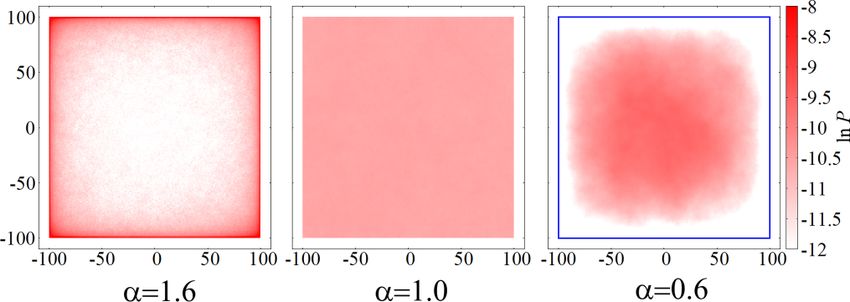
THOMAS VOJTA et al. PHYSICAL REVIEW E 102, 032108 (2020)
10-3
α (from top) t
10 5 α = 1.6 α = 0.8
1.8 212 -2
16 10
1.6 2
18
4
1.3 2
10 20
1.0 10-4 2
22
2
0.8 224
103
α
-3
P
0 0.5 1 1.5 2 10
0.25 -5
2 10
10 st 0.2
0.15
101 0.1
10-4
0.05 -6
0
10
0
10 0 1 2 3 4 5 6 7
10 10 10 10 10 10 10 10 -4 -2 0 2 4 -400 -200 0 200 400
t x/104 x
FIG. 1. Mean square displacement x 2 on the interval FIG. 2. Log-linear plots of the probability density P vs position x
(−L/2, L/2) with L = 1000 for several α. The data are averages for α = 1.6 and 0.8 at several times t. The particles start at the center
over 10 000 particles starting at x = 0. The reflecting walls of intervals of length L = 105 and 103 , respectively. Each distribution
are implemented by using Eq. (9). The dashed line marks the is based on at least 105 particles. To improve the statistics, P is
value L 2 /12 ≈ 83 333 expected for a uniform distribution of averaged over a small time interval around each of the given times.
particles over the interval, and the dash-dotted line marks the The statistical errors of P are smaller than the symbol size.
value L 2 /4 = 250 000 expected if all particles collect at the walls.
The solid lines are fits of the initial time evolution to x 2 ∼ t α .
Inset shows the normalized stationary mean-square displacement is proportional to L 2 . [This also follows from the scaling
A(α) = x 2 st /L 2 vs the anomalous diffusion exponent α using law (15) discussed below]. The inset of Fig. 1 indicates that
interval lengths between L = 100 for α = 0.3 and L 10 000 for A(α) = x 2 st /L 2 evolves smoothly with α from the value 41
the largest α. The open squares mark the values expected in the expected in the ballistic limit α → 2 (where all particles get
limits α → 0 and α → 2. The statistical errors of x 2 st /L 2 are much stuck directly at the walls) to the value 0 for α → 0 (where
smaller than the symbol size. the particles do no leave the center). The crossover time
tx between anomalous diffusion and saturation follows from
σ 2txα = A(α)L 2 .
walls at both ends. They established that, for all α = 1, the We emphasize that the functional behavior of the stationary
stationary probability density P(x) deviates from the uniform mean-square displacement shown here is strikingly different
distribution observed for normal Brownian motion. For α > 1, from the one obtained for FBM in a harmonic confining po-
the probability density is increased at the walls and reduced in tential, represented by a force F (x) = −bx in Eq. (11). (Note
the middle of the interval. For α < 1, the opposite behavior that FBM does not fulfill a fluctuation-dissipation relation and
is observed. However, the functional form of the probability is thus not thermalized). There, the mean-square displacement
density on a finite interval has not yet been studied systemati- takes the value x 2 harm = 21 σ 2 b−α (α + 1) [53]. In particu-
st
cally. 2 −α
lar, the value of x 2 harm
st /(σ b /2) is unity for α → 0 and
In the rest of this section, we therefore analyze one-
at α = 1, attains its minimum of about 0.89 at α ≈ 0.46, and
dimensional FBM on long intervals of lengths L σ , with
reaches its maximum of two in the ballistic limit α → 2.1
reflecting walls at both ends. We use up to 229 time steps.
We now turn to the time evolution of the probability density
This allows us to determine the probability density and, in
function P(x, t ). Figure 2 shows the probability density for
particular, analyze its functional form close to the walls.
α = 1.6 and 0.8 at several different times. At early times, it is
In addition, we carefully study the effects of different wall
not affected by the walls and takes a Gaussian form, just as for
implementation on the probability density.
free FBM. Once the distribution interacts with the reflecting
walls, particles start to accumulate close to the walls in the
B. Reflected fractional Brownian motion on a finite interval superdiffusive case α = 1.6 while P remains suppressed at
the walls for the subdiffusive case α = 0.8. The probability
We first study the time evolution of the mean-square dis-
density reaches a nonuniform stationary state for times larger
placement x 2 of FBM on the interval (−L/2, L/2). The
than approximately 222 .
particles start at the origin, i.e., in the center of the interval.
It is interesting to compare the form of the stationary
Figure 1 presents the mean-square displacement for an in-
probability density P for different interval lengths L. Figure 3
terval of length L = 1000 for several different anomalous
presents the corresponding simulation data for several L be-
diffusion exponents α. The figure demonstrates that x 2
tween 100 and 105 using scaled variables PL vs x/L. The
initially grows following the same t α power law as unconfined
curves for different L collapse nearly perfectly onto a common
FBM. At long times it saturates at a stationary value x 2 st that
changes with α, suggesting a nonuniform and α-dependent
distribution of particles in the stationary state. In the contin-
uum limit L σ , the stationary mean-square displacement 1
These relations hold in the continuum limit x 2 harm
st σ 2.
032108-4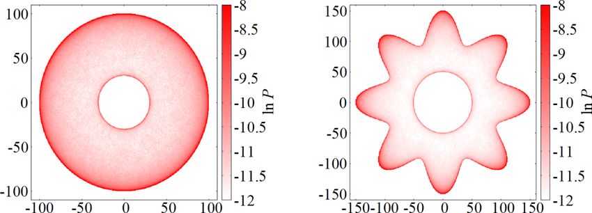
REFLECTED FRACTIONAL BROWNIAN MOTION IN ONE …                                                             PHYSICAL REVIEW E 102, 032108 (2020)

                                                                                2
                                                                               10
                                                            L                                                                2

     10                                                     100                                                              1
                                                            400

                                                                                                                         κ
               α=1.6                                       1600                 1
                                                                               10                                            0
                              α=0.8                        6400
                                                                                                                             -1
     3                                                    25600                         α (l.h.s. from top)                       0.5          1           1.5
PL

                                                                                                                                                    α

                                                                         PL
                                                         100000                 0
                                                                                                   1.8
                                                                               10                  1.6
                                                                                                   1.3
     1
                                                                                                   1.2
                                                                           10-1                    1.0
                                                                                                   0.8
  0.3                                                                                              0.5
    -0.5 -0.4 -0.3 -0.2 -0.1         0    0.1   0.2   0.3   0.4    0.5                         10-3                  10-2                    10-1                   100
                                    x/L                                                                                (x-w)/L

   FIG. 3. Scaling plot of the stationary probability density showing         FIG. 4. Scaled stationary probability density PL vs scaled dis-
PL vs x/L for α = 1.6 and α = 0.8 for several interval length L.          tance (x − w)/L from the wall for several α. The system sizes
Each distribution is based on 104 to 105 particles; P is averaged over    range from L = 200 for α = 0.5 to L = 106 for the largest α. Each
a number of time steps after a stationary state has been reached.         distribution is based on 104 to 105 particles; P is averaged over a
                                                                          large number (up to 225 ) of time steps after a stationary state has been
                                                                          reached. Inset shows exponent κ extracted from power-law fits of
master curve, demonstrating that the stationary distribution              P(x) close to the wall. The solid line is the conjecture κ = 2/α − 2.
fulfills the scaling form
                                                                                                C. Influence of wall implementation
                                   1
                       P(x, L) =     Yα (x/L)                     (15)        In this section, we carefully study how different implemen-
                                   L
                                                                          tations of the reflecting walls (see Sec. II B) affect the proba-
with high accuracy. Small deviations (almost invisible in the             bility density of FBM on a finite interval. Figure 5 presents
figure) can be attributed to finite-size effects close to the wall        example trajectories produced by the same noise sequence
that vanish in the continuum limit L         σ . We have carried          using boundary conditions (8)–(11). The figure shows that
out similar simulations for other values of the anomalous                 the differences between these trajectories are of the order of
diffusion exponent α. All data fulfill the scaling relation (15)          the step size σ while they become indistinguishable on length
but the functional form of the dimensionless scaling function             scales large compared with σ .
Yα (z) depends on α. Note that the scaling form (15) also                     To analyze the effects of the wall implementation quan-
implies that the probability density of FBM on an interval                titatively, we compare in Fig. 6 the stationary probability
of fixed length becomes independent of the step size σ in
the limit σ → 0, guaranteeing that our reflected FBM has a
                                                                                                                                  rFBM, xn+1= xn + ξn + F(xn)
proper continuum limit.                                                                                                           rFBM, xn+1= | xn + ξn |
    Let us now focus on the behavior of the stationary prob-                                                                      rFBM, xn+1= max(xn+ξn, 0)
                                                                               100
ability density close to the reflecting walls. Based on the                                                                       rFBM, xn+1= xn + ξn (if xn + ξn > 0)
results for reflected FBM on a semi-infinite interval [38,39],                                                                         xn+1= xn (otherwise)

we expect the probability density to feature a power-law
singularity at the wall. In Fig. 4, we therefore present a
                                                                                    0
double-logarithmic plot of the probability density as a func-                                                 t
                                                                                        2500       2520           2540       2560
tion of the distance from the reflecting wall for several α
                                                                         x

                                                                                                                               6
between 0.5 and 1.8. The figure shows that all curves
become straight lines close to the wall, indicating that the                                                                       4                      free FBM
stationary probability density indeed follows the power-law                -100
                                                                                                                                   x

P ∼ (x − w)κ . We determine the values of the exponent κ                                                                           2
by power-law fits of the probability density close to the wall
but outside of the region influenced by finite-size effects,                                                                       0
i.e., for σ     x−w       L. The inset of Fig. 4 shows κ as                -200
                                                                               0                      1000               2000                 3000                4000
a function of α. The exponent follows the conjecture κ =                                                                   t
2/α − 2 with high accuracy, i.e., it takes the same values
as the exponent in the case of a semi-infinite interval. This                FIG. 5. Example trajectories of FBM (α = 1.2) with a reflecting
implies that the scaling function Yα in Eq. (15) behaves as               wall at the origin (rFBM), implemented via the boundary conditions
Yα (z) ∼ (z + 1/2)κ = (z + 1/2)2/α−2 for z + 1/2          1 (close        (8)–(11). For the soft wall (11), the force parameters are F0 = 0.5
to the left interval boundary) and analogously for the right              and λ = 1. The free FBM trajectory is shown for comparison. Inset:
boundary.                                                                 Zoomed-in view of the trajectories very close to the wall.

                                                                    032108-5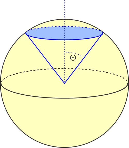
THOMAS VOJTA et al. PHYSICAL REVIEW E 102, 032108 (2020)
10-2 the repulsive force (12) with amplitude F0 = 0.2 and decay
boundary condition constant λ = 0.2. The left panel, Fig. 7(a), indicates that
"inelastic" (particle stops) the width of the wall region (marked by the dashed line) is
"elastic" (instantaneous reflection)
10
-3
repulsive force, F0=1.0, λ=0.2
independent of the interval lengths. This implies that the wall
repulsive force, F0=0.2, λ=0.2 region becomes unimportant for L σ, L λ−1 . Indeed, the
right panel, Fig. 7(b), shows that the same data, plotted in
10
-4
scaled variables PL vs (x − w)/L, collapse onto a common
P
master curve for x outside of each of the respective wall
regions.
10-5 These results demonstrate that variations of the probability
density due to different implementations of the reflecting
walls can be considered finite-size effects that vanish in the
10-6 continuum limit L/σ → ∞, Lλ → ∞. A rigorous proof that
100 101 102 103 104 105 106
the discretization error vanishes in the continuum limit was
x-w
given in Ref. [54] for the wall implementation (10).
Note that, inside the wall region (distances of order σ
FIG. 6. Stationary probability density P vs distance x − w from from the wall), some implementations of the reflecting bound-
the wall for α = 1.6, L = 106 and several implementations of the ary are better behaved than others and converge faster to
reflecting walls. Each distribution is based on 105 particles; P is the continuum limit, as was shown for normal diffusion in
averaged over a large number of time steps in the stationary regime. Refs. [55,56]. For example, we observed in Ref. [40] that
The dotted line is a power-law fit. the wall implementation (10) leads to stronger discretization
artifacts than rule (8). However, all of these artifacts vanish in
the continuum limit.
densities P(x) for “elastic” walls (8), “inelastic” walls (9), and
This differs from the behavior of the fractional Langevin
walls implemented via “soft” repulsive forces (12) with two
equation with reflecting walls where recent computer simu-
different amplitudes for a finite interval of length L = 106 and
lations [57] have shown that the implementation of the wall
α = 1.6. The data show that the wall implementation indeed
appears to affect the probability density in the entire interval,
influences the probability density in the immediate vicinity of
perhaps due to a subtle interplay of the boundary conditions
wall. For example, a strong repulsive force pushes the peak
and the fluctuation-dissipation theorem that establishes ther-
of P(x) away from the nominal wall position. However, the
mal equilibrium.
figure also demonstrates that all four wall implementations
produce exactly the same probability density further away
from the wall. D. Fractional Brownian motion in superharmonic potentials
To investigate in more detail the region in which the
In this section, we briefly address the behavior of FBM
wall implementation affects P(x), we compare the results
that is confined to a finite interval not by reflecting walls but
for different interval lengths. Figure 7 presents the stationary
by a smooth external potential. The goal is to further under-
probability density for α = 1.6 for intervals having lengths
line that the observed accumulation and depletion effects are
from L = 1600 to 106 employing “soft” walls defined by
neither artifacts of the specific reflecting boundary conditions
considered in the remainder of this paper, nor due to the
(a) 10-2 (b) implementation of the fractional Gaussian noise (the noise
3 L= sequence, once simulated, is used as input continuously, no
10
1600
104
matter whether a reflection takes place or not). For a harmonic
10
-3 10
5 potential U (x) ∝ x 2 , FBM can be solved exactly and was
2
10
6
analyzed in detail in Refs. [45,53]. In particular, the proba-
10 bility density remains Gaussian in this case. However, if we
10-4 consider somewhat steeper potentials, for instance, the quartic
PL
P
form U (x) ∝ x 4 , distinct deviations from the naively expected
101 Boltzmann form P(x) ∝ exp(−ax 4 ) can be observed. In this
-5
10 case, the time evolution of the process can be obtained from
the discrete Langevin equation (11) with F (x) = −dU/dx.
To study FBM in a quartic potential, we perform simu-
100
10-6 lations of the recursion relation (11) using a force F (xn ) =
100 102 104 106 10-6 10-4 10-2 100
−kxn3 and a noise variance of σ 2 = α , with k = 0.2 and =
x-w (x-w)/L
0.002. Figure 8 shows the resulting stationary probability den-
sity for different α. In the case of normal Brownian motion,
FIG. 7. (a) Stationary probability density P vs distance x − w α = 1, the Boltzmann form is reproduced very well. How-
from the wall for α = 1.6, and several interval lengths. The walls ever, relative to the Boltzmann law, the probability density
are implemented as repulsive forces (12) with F0 = 0.2 and λ = 0.2. near the points of highest curvature of the external potential
The dashed line marks the widths of the wall region. (b) The same is increased for superdiffusive FBM (α > 1) and decreased
data plotted in scaled variables PL vs (x − w)/L. for the subdiffusive case (α < 1). These observations are
032108-6REFLECTED FRACTIONAL BROWNIAN MOTION IN ONE … PHYSICAL REVIEW E 102, 032108 (2020)
100
10-1
P
FIG. 10. Heat maps of the stationary probability density P for
α α = 1.6, computed from 100 particles performing up to 221 time
0.2 steps.
-2 1.0
10 1.4
2.0 Analogous accumulation and depletion effects are also
-2 -1.5 -1 -0.5 0 0.5 1 1.5 2 observed in other geometries. Figure 10 shows heat maps of
x the stationary probability density of FBM on a ring-shaped
domain and a star-shaped domain for α = 1.6 in the superdif-
FIG. 8. Stationary probability density P of FBM in a quartic fusive regime. These shapes allow us to analyze the differ-
potential U (x) ∝ x 4 for several values of α. Each distribution is based ences between concave and convex boundaries. As above, the
on 5000 time steps, averaged over 500 000 trajectories. For normal data indicate that particles accumulate close to all reflecting
Brownian motion, α = 1, the Boltzmann distribution (heavy black walls. The accumulation is stronger for concave boundaries
line) fits the simulation results very well, whereas in the sub- and such as the outer boundary of the ring and weaker for convex
superdiffusive cases, respectively, depletion and accumulation with boundaries such as its inner boundary.
respect to the Boltzmann law are observed close to the points of
highest curvature of U (x).
B. Rectangular domains
We now analyze the probability density of reflected FBM
fully consistent with our results for the reflecting boundary in two-dimensional geometries quantitatively. Square and
conditions. rectangular domains are particularly simple cases because
the motions parallel and perpendicular to the walls, i.e.,
IV. TWO SPACE DIMENSIONS the x and y components of the two-dimensional FBM for
appropriately chosen coordinate axes, completely decouple.2
A. Overview The two-dimensional probability density is therefore simply a
Let us now turn to reflected FBM in two dimensions. product of two one-dimensional probability density functions.
We have performed simulations for a variety of geometries. Specifically, for a rectangle of sides Lx and Ly , the stationary
For a qualitative overview, we present in Fig. 9 heat maps probability density takes the form
of the stationary probability density of FBM confined to a
P2d (x, Lx ; y, Ly ) = P1d (x, Lx )P1d (y, Ly ) (16)
square domain by reflecting walls. The figure compares three
different values of the anomalous diffusion exponent, viz., in the continuum (scaling) limit Lx , Ly σ . Here, P1d (x, Lx )
α = 1.6 (superdiffusive regime), α = 1 (normal Brownian and P1d (y, Ly ) are the stationary distributions of one-
motion), and α = 0.6 (subdiffusive regime). The data indicate dimensional FBM on finite intervals of length Lx and Ly ,
the same qualitative behavior as observed in one dimension. respectively.
In the superdiffusive regime, particles accumulate close to This has the following implications for behavior of the sta-
the reflecting boundaries, compared with the flat distribution tionary probability density at the boundaries of the rectangular
for normal diffusion. In the subdiffusive regime, in contrast, domain. When the edge of the rectangle is approached away
particles are depleted close to the walls. The strongest accu- from a corner, the probability density features a power-law
mulation and depletion are seen in the corners of the square. singularity with the same exponent value, κ = 2/α − 2, as
in one dimension. In contrast, if the corner of the rectangle
is approached along the diagonal (or any other straight line),
the probability density follows a power-law with the doubled
exponent κ = 4/α − 4. Consistently, relatively higher densi-
ties are observed close to the corners. We have confirmed
this explicitly by computer simulations on square domains for
anomalous diffusion exponents α = 0.8, 1.2, 1.4, and 1.6.
2
x and y may be coupled during the reflection process for some
FIG. 9. Stationary probability density P of FBM on a square choices of the reflection condition. Based on the results of Sec. III C,
domain for several α. The heat maps of ln P are based on 100 this is not expected to influence the probability density outside the
particles performing up to 224 time steps each. narrow “wall region.”
032108-7THOMAS VOJTA et al. PHYSICAL REVIEW E 102, 032108 (2020)
2
outer boundary
101 1 inner boundary
101
κ
0
-1
α (l.h.s. from top)
P Rmax
0.5 1 1.5
P R2
100 α
2
1.8 100
1.6
1.4
1.2
-1
10 1.0 10-1
0.8
0.6
-3 -2 -1 0 -3 -2 -1 0
10 10 10 10 10 10 10 10
(R-r)/R (Rmax-r)/Rmax , (r-Rmin)/Rmax
FIG. 11. Stationary probability density P(r) of FBM on circular FIG. 12. Scaled stationary probability density on a ring with
domains (disks) of radius R for several α. The data are plotted as outer radius Rmax = 106 and inner radius Rmin = 0.3Rmax vs scaled
PR2 vs scaled distance (R − r)/R from the wall. System sizes range distance from both boundaries for α = 1.6. The simulations use 105
from R = 106 for α = 1.8 to R = 1000 for α = 0.6; the simulations particles performing 227 time steps. The dashed lines are fits to power
use 104 to 105 particles and up to 229 time steps. Inset shows the laws with the conjectured exponent κ = 2/α − 2 = −0.75.
exponent κ extracted from power-law fits of P(r) close to the wall.
The solid line is the one-dimensional conjecture κ = 2/α − 2.
ring for superdiffusive FBM. However, the accumulation is
stronger at the concave outer boundary than at the convex
C. Disks and rings
inner boundary. Figure 12 presents a quantitative analysis of
For FBM on domains with curved boundaries, such as a the probability density close to both walls for α = 1.6. Close
circular domain (disk) of radius R, the situation is more com- to the outer boundary, the probability density clearly follows
plicated. For uncorrelated or short-range correlated random the conjectured power law P ∼ (Rmax − r)2/α−2 . At the inner
walks, one would expect the curvature of the boundary to boundary we observe a much slower crossover, but the data
become unimportant if the radius R of the curvature is large are compatible with an asymptotic power-law singularity with
compared with the step size σ (or the finite correlation length the same exponent, P ∼ (r − Rmin )2/α−2 .
of the steps). However, FBM has long-range correlations and
thus effectively sees (remembers) the entire domain. It is
D. Circular sectors
therefore not clear a priori whether the curvature affects the
behavior of the probability density near the boundary. The results of the last section show that the curvature of
To resolve this question, we perform extensive simulations a reflecting wall does not influence the qualitative behavior
of FBM on large circular domains with radii up to R = 106 of the probability density close to the wall. However, the
for anomalous diffusion exponents α between 0.6 and 1.8. example of a square domain in Sec. IV A indicates that sharp
We find that the stationary probability density is, of course, corners lead to stronger singularities of the probability density
rotationally invariant, i.e., independent of the polar angle. Its at the boundary.
radial dependence fulfills the scaling form In the present section, we study this effect systematically
by performing simulations of FBM on circular sectors of
1
P2d (r, R) =Yα (r/R) (17) radius R and varying opening angle for anomalous diffusion
R2 exponents α = 1.6 (superdiffusive regime) and 0.8 (subdif-
for R σ . Here, r is the distance from the center of the fusive regime). Two examples that illustrate the geometry of
disk. Figure 11 summarizes the results of these simulations, these sectors are presented in Fig. 13. For α = 1.6, the heat
focusing on the behavior of the probability density P close to map of the probability density of the 60◦ sector in Fig. 13
the reflecting boundary at r = R. It shows that P behaves as shows a particularly strong accumulation in the tip (center of
a power of the distance from the wall for all α. We determine curvature) of the sector.
the exponent from fits of the power law P(r) ∼ (R − r)κ to the To understand quantitatively the behavior in the tip, we
probability density close to the wall but outside of the region analyze the stationary probability density along the symmetry
influenced by finite-size effects, i.e., for σ R−r R. The line (dashed line in Fig. 13) of the sector. Figure 14 shows
inset of Fig. 11 shows the resulting values of the exponent κ as a double-logarithmic plot of the (scaled) probability density
a function of α. They follow the same conjecture κ = 2/α − 2 as a function of the distance from the tip. All curves feature
as in the one-dimensional case, suggesting that the curvature power-law behavior for r R but the exponent changes con-
of the reflecting wall does not affect the functional form of the tinuously with the opening angle of the sector. The inset of
probability density near the wall. Fig. 14 presents the values of the exponent, determined from
In addition to disks, we also consider ring-shape domains. fits of the probability density by P(r) ∼ r κ for σ r R.
As was already shown in the heat map in Fig. 10, particles We observe that the divergence of P(r) becomes stronger
accumulate at both the inner and the outer boundary of the (κ becomes more negative) as the opening of the sector
032108-8REFLECTED FRACTIONAL BROWNIAN MOTION IN ONE … PHYSICAL REVIEW E 102, 032108 (2020)
1
10
Θ (bottom to top)
30o
o
60
10
0
90o
o
120
o
180
Θ
2
PR
240o 0 90 180 270 360
-1 o
10 300 2
1.5
FIG. 13. Heat maps of the stationary probability density of FBM
κ
1
(α = 1.6) on circular sectors with opening angles = 60◦ and 240◦ . 10-2
The simulations use 100 particles performing 218 time steps. The 0.5
dotted line marks the cut used to analyze the singularity of the PDF
in the tip (corner) at the center of the curvature. 10-2 10-1 100
r/R
gets narrower. For = 180◦ , κ takes the value 2/α − 2 as FIG. 15. Scaled stationary probability density PR2 of FBM with
α = 0.8 on a circular sector with outer radius R = 103 for various
on a one-dimensional interval. This is expected because the
opening angles . The graphs show PR2 on the symmetry line of
left boundary of the sector is a straight line for = 180◦ .
the sector as a function of the scaled distance r/R from the center
Similarly, we find κ = 4/α − 4 for = 90◦ , as in the corner
of curvature (106 particles performing 225 time steps). Inset shows
of a square. For → 360◦ , the exponent κ approaches a value the exponent κ extracted from power-law fits, P(r) ∼ r κ , of the PDF
close to −0.5. At first glance, one might have expected κ to close to the center (r/R 1) vs opening angle . The dashed lines
approach zero in this limit because the probability density of mark the values 2/α − 2 = 0.5 and 4/α − 4 = 1.0.
a disk does not have a singularity in the center. Note, however,
that a reflecting line along the negative x axis remains in the
→ 360◦ limit of the sector. of the wall implementation do not affect the results, we also
We also carry out analogous simulations for subdiffusive perform simulations using soft walls, defined by appropriate
FBM using α = 0.8. The results are presented in Fig. 15. As generalizations of Eqs. (11) and (12) to the circular sector
above, the deviations from a flat distribution become stronger geometry. Specifically, we have analyzed sectors with open-
as the opening angle of the sector decreases. For = 180◦ ings of 15◦ and 90◦ for α = 1.6 in this way. As in one
and = 90◦ , we recover the expected exponent values κ = dimension (Sec. III C), we find that the wall implementation
2/α − 2 and 4/α − 4, respectively. only influences a narrow “interaction region” close to the wall
The results in this section are obtained by using the “in- that becomes unimportant in the continuum (scaling) limit
elastic” boundary conditions (13). To confirm that the details R/σ → ∞.
V. THREE SPACE DIMENSIONS
5
10 -0.5 In this section, we briefly discuss reflected FBM in
three-dimensional geometries. Domains shaped as rectangular
-1
prisms (cuboids) can be analyzed analogously to Sec. IV B.
κ
Because the x, y, and z components of a three-dimensional
3 -1.5
10 FBM are independent of each other, the stationary probability
Θ (top to bottom)
30o 0 90 180 270 360 density of FBM in a rectangular prism of sides Lx , Ly , and Lz
2
PR
o Θ factorizes and takes the form
90
120o
101 P3d x, Lx ; y, Ly ; z, Lz = P1d (x, Lx )P1d y, Ly P1d (z, Lz ) (18)
150o
180o in an appropriate coordinate system having axes parallel to the
210o edges of the prism. This implies that the probability density
300o features a power-law singularity with exponent 2/α − 2 when
10-1
-4 -3 -2 -1 0
a face of the prism is approached. If an edge is approached
10 10 10 10 10
the exponent is given by 4/α − 4, and when a corner is
r/R
approached (along a straight line) the exponent is expected
FIG. 14. Scaled stationary probability density PR2 of FBM with to be 6/α − 6.
α = 1.6 on circular sectors with outer radius R = 105 and various Turning to spherical domains, we simulate superdiffusive
opening angles . The graph shows PR2 on the symmetry line of the FBM with α = 1.6 in a sphere of radius R = 106 and sub-
sector as a function of the scaled distance r/R from the center of cur- diffusive FBM with α = 0.8 in a sphere of radius R = 103 .
vature. (105 to 106 particles performing 223 time steps.) Inset shows We observe that the behavior of the stationary probability
the exponent κ extracted from power-law fits, P(r) ∼ r κ , of the data density is completely analogous to the case of a circular (disk)
close to the center (r/R 1) vs opening angle . The dashed lines domain discussed in Sec. IV C. Specifically, the probability
mark the values 2/α − 2 = −0.75 and 4/α − 4 = −1.5. density features a power-law singularity at the surface of the
032108-9THOMAS VOJTA et al. PHYSICAL REVIEW E 102, 032108 (2020)
3
2.5
101 2
1.5
κ
1
0.5
0 Θ (bottom to top)
100
3
PR
0 30 60 90 120 150 180 o
Θ
15
30o
o
45
10-1 60o
o
75
90o
o
-2 120
10
FIG. 16. Geometry of the spherical cone. 10-2 10-1 100
r/R
sphere that is controlled by the one-dimensional exponent FIG. 18. Scaled stationary probability density PR3 of FBM with
κ = 2/α − 2. α = 0.8 in a spherical cone with outer radius R = 103 for various
To determine how the “sharpness” of a corner affects the opening angles . The graphs show PR3 on the symmetry line of the
probability density in three dimensions, we simulate FBM in cone as functions of r/R (106 particles performing 225 time steps).
spherical sectors (spherical cones) of variable opening angles Inset shows the exponent κ determined from power-law fits, P(r) ∼
for α = 1.6 and 0.8. A spherical cone contains all points r κ , of the data close to the center (r/R 1) vs opening angle . The
whose distance from the origin is less than R and whose polar dashed line marks the value 2/α − 2 = 0.5.
angle is less than , see Fig. 16. We then analyze the proba-
bility density on the symmetry axis of the cone. The results for
superdiffusive motion with α = 1.6 are presented in Fig. 17 P) because particles can easily go around the repulsive line
for several opening angles of the cone. As in the case along the negative z axis remaining in this limit (in contrast
of circular sectors, all curves feature power-law singularities with the two-dimensional case).
close to the tip (center of curvature) of the cone. We determine Figure 18 presents the same analysis for subdiffusive mo-
the exponents from fits of the probability density to P(r) ∼ r κ . tion with α = 0.8. We again observe power-law singularities
The resulting values are presented in the inset of Fig. 17 as a in the probability density close to the tip of the cone, with an
function of the opening angle . For = 90◦ , κ takes the exponent that increases continuously as the cone narrows. The
one-dimensional value 2α − 2 because the reflecting wall at values of the scaling exponent, determined from power-law
the bottom of the cone is completely flat. For → 180◦ , the fits, are shown in the inset of the figure. As expected, for
exponent κ approaches zero (corresponding to a nonsingular = 90◦ , we recover the one-dimensional exponent 2/α − 2.
0 VI. APPLICATION TO BRAIN SEROTONERGIC FIBERS
8 -0.5
10 As was pointed out in the introductory section of this
-1
paper, FBM has found a broad variety of applications in
κ
-1.5
6
10 -2 physics, chemistry, biology, and beyond. Recently, it has been
-2.5 proposed that FBM may be a good model for the geometry
Θ (top to bottom)
104
0 30 60 90 120 150 180 of serotonergic fiber paths in vertebrate brains, including the
3
o
PR
15 Θ
human brain.
30o
2 45
o The entire central nervous system of vertebrates is per-
10
60o meated by a dense network of serotonergic fibers, very long
75
o axons of neurons that are located in the brainstem [58,59].
100 90o These fibers release the neurotransmitter serotonin as well
120o as other neurotransmitters. The densities of this serotoner-
-2
10 -4 gic matrix vary significantly across brain regions, and their
10 10-3 10-2 10-1 100
perturbations can severely affect the function of neural cir-
r/R
cuits. Traditionally, the emergence of these densities has been
FIG. 17. Scaled stationary probability density PR3 of FBM with treated as a tightly controlled sequence of developmental
α = 1.6 in a spherical cone with outer radius R = 105 for various events that reflects the functional requirements of individual
opening angles . The graphs show PR3 on the symmetry line of brain regions (neuroanatomical nuclei and laminae). Based on
the cone vs the scaled distance r/R from the center of curvature high-resolution imaging techniques (see Fig. 19), it has been
(107 particles performing 223 time steps). Inset shows the exponent suggested, however, that individual fibers behave as three-
κ determined from power-law fits, P(r) ∼ r κ , of the data close to dimensional stochastic processes, with the varying fiber densi-
the center (r/R 1) vs opening angle . The dashed line marks the ties emerging from the interaction of the randomness with the
value 2/α − 2 = −0.75. complex brain geometry [41,60]. Specifically, superdiffusive
032108-10REFLECTED FRACTIONAL BROWNIAN MOTION IN ONE … PHYSICAL REVIEW E 102, 032108 (2020)
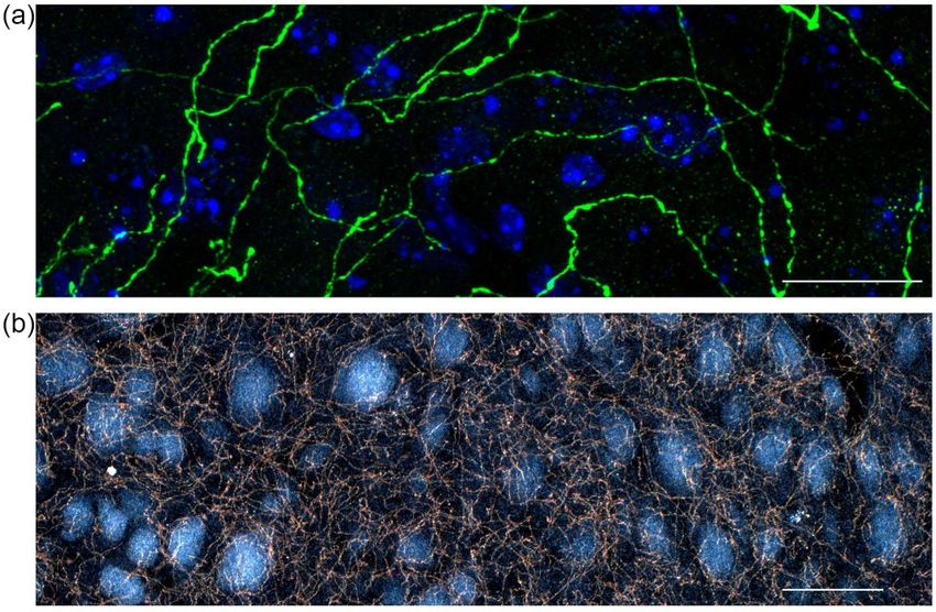
FIG. 19. (a) A confocal microscopy image of serotonergic fibers
visualized with an anti-GFP antibody in the cingulate cortex (area 30)
of the transgenic mouse model developed by Migliarini et al. [61].
The fibers are shown as green (bright) lines; cell nuclei are labeled
blue (dark gray). Scale bar = 20 μm (the thickness of the z stack FIG. 20. Serotonergic fibers in a cross section through the mouse
is 19 μm). (b) A dark-field microscopy image of serotonergic fibers midbrain. (a) Fiber densities visualized with an anti-serotonin-
visualized with an anti-serotonin-transporter antibody in the caudate- transporter antibody. Higher densities are darker in the image;
putamen of a wild-type mouse. The fibers are shown as golden brown individual fibers are not visible at this magnification. Aq, cere-
(light gray) lines. Scale bar = 100 μm. bral aqueduct; cp, cerebral peduncle; IPN, interpeduncular nucleus;
MGN, medial geniculate nucleus; ml, medial lemniscus; SC, superior
colliculus; SN, substantia nigra; vtgx, ventral tegmental decussation.
FBM has emerged as a promising theoretical framework for Scale bar = 1 mm. (b) Single fiber modeled as superdiffusive FBM
the description of brain serotonergic fibers [41,42]. trajectory of 217 steps with α = 1.6. (c) Heat map of the simulated
fiber density determined from 192 fibers of 223 steps each, plotted
Within this model, each individual serotonergic fiber is
as “optical” density exp(−βP) with β = 38 000. [The value of the
represented as a path of a discrete FBM with a step size related
attenuation parameter β was chosen such that the mean pixel value
to the thickness of the fibers (which determines how fast the
in the simulated section approximately matched the mean pixel value
fibers can bend). A comparison of FBM sample paths with of the actual section in panel (a)].
actual fiber trajectories suggests that appropriate values of the
anomalous diffusion exponent lie in the superdiffusive range.
Figure 20 presents an example of a computer simulation of This phenomenon is easy to understand qualitatively. If
this model applied to a section of a mouse brain. The figure the correlations are persistent (superdiffusive FBM), particles
clearly shows that the simulations reproduce the increased will attempt to continue in the same direction upon reaching
fiber densities observed at the boundaries of the real brain the wall and thus get trapped for a long time,3 increasing
section as well as in the concave parts of its geometry. the probability density near the wall. If the correlations are
A systematic study of this model and a detailed comparison antipersistent (subdiffusive FBM), particles will preferably
with the fiber densities in real mouse brains was carried out move away from the wall right after hitting it, reducing the
in Ref. [42]. The agreement of the simulated densities and probability density at the wall. (We emphasize that the noise
the densities determined from the mouse brain sections was correlations extend beyond the reflection events because the
found to be quite remarkable, especially in view of how little noise is externally given).
neurobiological input the model requires. Moreover, the study We note that these accretion and depletion effects arise
demonstrated that soft fiber-wall interactions can be partic- from the nonequilibrium nature of FBM. The fractional
ularly appropriate for modeling the behavior of serotonergic Langevin equation, which contains the same fractional noise
fibers in brain tissue. as FBM but fulfills the fluctuation-dissipation theorem [63],
reaches a thermal equilibrium stationary state that is gov-
erned by the Boltzmann distribution. On a finite interval
VII. CONCLUSIONS with reflecting walls, this leads to a flat probability density,
as was recently confirmed by large-scale simulations [57].4
In summary, we have performed large-scale computer sim-
The key role played by the fluctuation-dissipation theorem
ulations of FBM in one, two, and three dimensions in the pres-
ence of reflecting boundaries that confine the motion to finite
regions in space. In all studied geometries, we have found
that the stationary probability density deviates strongly from 3
The probability of finding long periods of motion in predomi-
the flat distribution observed for normal Brownian motion. nantly one direction is discussed in Ref. [62] for power-law corre-
Specifically, we have found particles to accumulate close to lated disorder.
4
the reflecting walls for superdiffusive FBM whereas they are The fractional Langevin equation does show accretion and deple-
depleted near the walls for subdiffusive FBM. tion effects, albeit weaker ones, in nonstationary situations [57].
032108-11THOMAS VOJTA et al. PHYSICAL REVIEW E 102, 032108 (2020)
becomes clear if one considers a generalized Langevin equa- supporting the use of FBM rather than a fractional Langevin
tion with long-time correlated fractional Gaussian noise but equation.
instantaneous damping. For this equation, which violates the Recently, the logistic equation with temporal disorder,
fluctuation-dissipation theorem, simulations [57] have shown which describes the evolution of a biological population
that the stationary probability density on a finite interval is not density ρ under environmental fluctuation, was mapped onto
uniform but resembles the corresponding result for FBM. FBM with a reflecting wall at the origin [64,65]. This mapping
Our simulations have demonstrated that the stationary relates the density of individuals and the position of the walker
probability density of FBM on a finite one-dimensional inter- through ρ = e−x . Consequently, the power-law singularity in
val features a power-law singularity, P(x) ∼ |x − w|κ , close the probability density of FBM is intimately tied to the critical
to a reflecting wall at position w. The exponent κ follows the behavior of the nonequilibrium phase transition between ex-
conjecture κ = 2/α − 2 [38] with high accuracy. In higher di- tinction and survival of the population and the dependence of
mensions, the stationary probability density close to a smooth its universality class on the correlations in the environmental
boundary (be it straight or curved) features a power singularity fluctuations [65].
governed by the same exponent, κ = 2/α − 2, as in one In many realistic systems, the power-law correlations are
dimension. Close to sharp (concave) corners, the singularities regularized beyond some time or length scale. To account for
are enhanced. When approaching the corner of a rectangle such regularization effects on the properties of confined FBM,
(along a straight line), the probability density features a power one can employ tempered fractional Gaussian noise [66].
law with exponent 4/α − 4, and for a general d-dimensional Finally, we emphasize that the combination of geometric
orthotope (hyperrectangle), the corresponding exponent is confinement and long-time correlations provides a general
expected to read 2d/α − 2d. route to a singular probability density. We therefore expect
We emphasize that all our results are robust against analogous results for many long-range-correlated stochastic
changes in how the reflecting walls are defined and imple- processes in nontrivial geometries.
mented. In Sec. III C, we systematically compare simulations
with four different types of reflecting boundary conditions.
These simulations demonstrate that details of the wall imple-
ACKNOWLEDGMENTS
mentation influence the probability density only in a narrow
“wall region” whose size is determined by the step size σ and This work was supported in part by a Cottrell SEED
becomes unimportant in the continuum limit L σ . For soft award from Research Corporation and by the National Sci-
walls, the size of the wall region is governed by the decay ence Foundation under Grants No. DMR-1828489 and No.
length of the wall force. OAC-1919789 (T.V.). S.J. acknowledges support by the Na-
The nonuniform and singular probability density of re- tional Science Foundation under Grants No. 1822517 and
flected FBM can have important consequences for applica- No. 1921515, by the National Institute of Mental Health
tions. One such application is the modeling of serotonergic (Grant No. MH117488), and by the California NanoSystems
fibers in the brain, as was discussed in Sec. VI. Here, the Institute (Challenge-Program Development grant). R.M. ac-
accretion and depletion of particles close to reflecting walls knowledges support from the German Research Foundation
and in concave parts of the geometry is crucial for correctly (DFG, Grant No. ME/1535/7-1) and from the Foundation
describing variations of the experimentally observed fiber for Polish Science (Fundacja na rzecz Nauki Polskiej, FNP)
densities in various brain regions. Note that active growth of within an Alexander von Humboldt Polish Honorary Research
these fibers in the brain is clearly not an equilibrium process, Scholarship.
[1] A. Einstein, Investigations on the Theory of the Brownian [12] B. B. Mandelbrot and J. W. V. Ness, SIAM Rev. 10, 422 (1968).
Movement (Dover, New York, 1956). [13] J. Szymanski and M. Weiss, Phys. Rev. Lett. 103, 038102
[2] M. von Smoluchowski, Z. Phys. Chem. 92U, 129 (1918). (2009).
[3] P. Langevin, C. R. Acad. Sci. Paris 146, 530 (1908). [14] M. Magdziarz, A. Weron, K. Burnecki, and J. Klafter, Phys.
[4] B. Hughes, Random Walks and Random Environments, Volume Rev. Lett. 103, 180602 (2009).
1: Random Walks (Oxford University Press, Oxford, 1995). [15] S. C. Weber, A. J. Spakowitz, and J. A. Theriot, Phys. Rev. Lett.
[5] R. Metzler and J. Klafter, Phys. Rep. 339, 1 (2000). 104, 238102 (2010).
[6] F. Höfling and T. Franosch, Rep. Prog. Phys. 76, 046602 (2013). [16] J.-H. Jeon, V. Tejedor, S. Burov, E. Barkai, C. Selhuber-Unkel,
[7] P. C. Bressloff and J. M. Newby, Rev. Mod. Phys. 85, 135 K. Berg-Sørensen, L. Oddershede, and R. Metzler, Phys. Rev.
(2013). Lett. 106, 048103 (2011).
[8] R. Metzler, J.-H. Jeon, A. G. Cherstvy, and E. Barkai, Phys. [17] J.-H. Jeon, H. Martinez-Seara Monne, M. Javanainen, and R.
Chem. Chem. Phys. 16, 24128 (2014). Metzler, Phys. Rev. Lett. 109, 188103 (2012).
[9] Y. Meroz and I. M. Sokolov, Phys. Rep. 573, 1 (2015). [18] S. M. A. Tabei, S. Burov, H. Y. Kim, A. Kuznetsov, T. Huynh, J.
[10] R. Metzler, J.-H. Jeon, and A. Cherstvy, Biochim. Biophys. Jureller, L. H. Philipson, A. R. Dinner, and N. F. Scherer, Proc.
Acta, Biomembr. 1858, 2451 (2016). Natl. Acad. Sci. USA 110, 4911 (2013).
[11] A. N. Kolmogorov, C. R. (Doklady) Acad. Sci. URSS (N.S.) [19] N. Chakravarti and K. Sebastian, Chem. Phys. Lett. 267, 9
26, 115 (1940). (1997).
032108-12You can also read