SCIENCEDIRECT - JIDONG ZHAO
←
→
Page content transcription
If your browser does not render page correctly, please read the page content below
Available online at www.sciencedirect.com
                                                   ScienceDirect

                                    Comput. Methods Appl. Mech. Engrg. 377 (2021) 113707
                                                                                                               www.elsevier.com/locate/cma

      Semi-coupled resolved CFD–DEM simulation of powder-based
            selective laser melting for additive manufacturing
                                                     Tao Yu, Jidong Zhao ∗
                            Hong Kong University of Science and Technology, Clearwater Bay, Kowloon, Hong Kong
                        Received 6 January 2021; received in revised form 23 January 2021; accepted 25 January 2021
                                                           Available online xxxx

Abstract
    We present a semi-coupled resolved Computational Fluid Dynamics (CFD) and Discrete Element Method (DEM) to simulate
a class of granular media problems that involve thermal-induced phase changes and particle–fluid interactions. We employ an
immersed boundary (IB) method to model the viscous fluids surrounding solid particles in conjunction with a fictious CFD
domain occupied by the actual positions of the particle. Heat transfers between the actual fluids and the fictitious particle are
treated as a multiphase problem by the CFD to resolve the temperature gradient distribution within each granular particle and
its possible phase change (e.g., melting or partial melting). The mechanical interactions between the solid particles and the
fluids are modeled by coupled DEM and CFD. The proposed method is validated by simulations of a typical powder-based
selective laser melting (PB-SLM) process. Three key SLM input parameters, laser power, laser energy distribution and hatch
distance, are examined on the effect of melting. The simulation results capture key features and observations of PB-SLM found
in experiments and are quantitatively consistent with available testing data. The study provides a physically based, high-fidelity
computational approach for future PB-SLM additive manufacturing.
⃝c 2021 Elsevier B.V. All rights reserved.

Keywords: Granular media; Coupled CFD–DEM; Immersed Boundary Method; Multiphase modeling; Selective laser melting; Additive
manufacturing

1. Introduction
   Additive manufacturing (AM), also widely known as 3D printing (3DP), has been widely considered as a
technology paving the way for the next industrial revolution towards the ultimate ‘direct digital manufacturing’
(DDM) [1]. It helps to eliminate various constraints in conventional manufacturing industries that hinder optimal
design, creativity and ease of manufacturing [2,3]. Among many, selective laser melting (SLM) represents a typical
powder-based additive manufacturing technology using high-power lasers to melt metallic powders layer by layer
to form a desired product. It features short manufacturing circle, low costs, better molding accuracy and mechanical
properties [4], and has seen great potentials for application in a wide range of engineering and industries, such as
the printing of aerospace components [5,6], biomedical implants [7,8]. and polymers [9]. Its future developments
and wide applications, however, hinge crucially upon overcoming a number of technical barriers, including the
  ∗ Corresponding author.
    E-mail address: jzhao@ust.hk (J. Zhao).

https://doi.org/10.1016/j.cma.2021.113707
0045-7825/⃝  c 2021 Elsevier B.V. All rights reserved.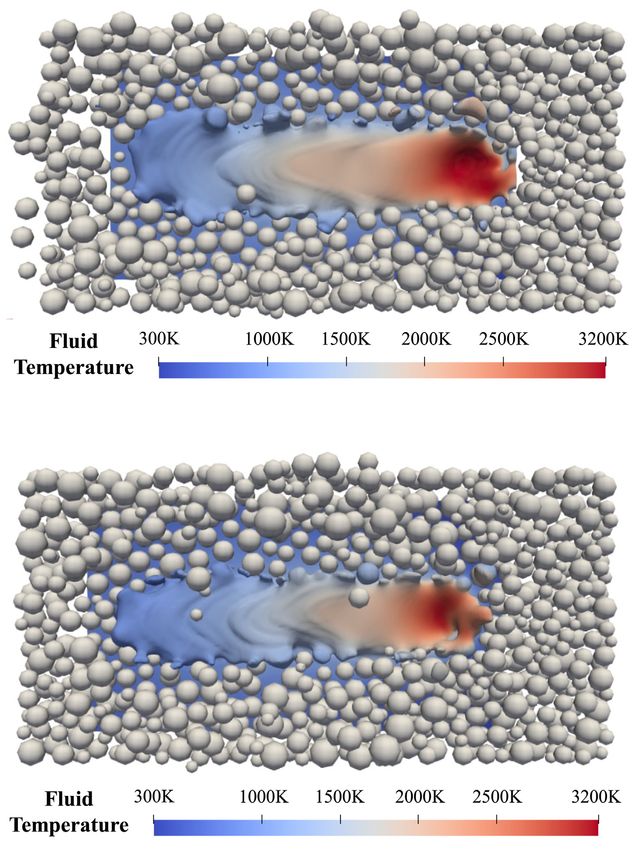
T. Yu and J. Zhao                                         Computer Methods in Applied Mechanics and Engineering 377 (2021) 113707

Table 1
Typical experimental studies of powder based SLM.
 Variables                           Typical specific factors
                                     Grain size distribution [27,28]                                 Powder layer thickness [29,30]
 Powder layer
                                     Radius ratio of laser and powder [28]                           Preheating temperature [31]
                                     Laser energy density [28,32,33]                                 Energy distribution [34]
 Laser beam
                                     Hatch distance [18,35]                                          Scanning strategy [36–39]
 Material type                       Printing materials (Aluminum, stainless steel, Ti-6Al-4V, inconel) [40,41]

poor surface roughness control caused by the balling effect, the spatter and “stair step” effect [10], and locally poor
mechanical properties of built parts [11] caused by pores [12], cracking, residual stresses, and distortion [13]. Both
experimental and numerical studies have been attempted to address these outstanding challenges in advancing the
SLM technology to new levels [14–17].
   The experimental studies have been focused on probing the printing effects of various controlling parameters
pertaining to the powder layer, laser beam and material type, such as laser scanning speed, layer thickness and
energy density [18,19], as summarized in Table 1. These tests indicate that low laser energy density may cause
undesirable high porosity, cracking and surface defects [20,21], while optimal energy density can help ensure
high quality melting of powders and formation of underlying base-plate bonding [22]. Excessive use of energy
density, however, may possibly amplify the material evaporation and spattering [23] and result in the formation of
pores in the built parts [24]. These experimental studies have helped to provide key insights into the understanding
and optimization of practical printing procedures for quality control of the built parts. Nevertheless, experimental
investigations of SLM commonly follows a trial and error approach which renders them costly, inefficient and
less rigorous [25]. Numerical simulations have become a popular alternative in providing cost-effective, repeatable,
systematic investigations of the entire manufacturing process for defect detection and facilitate seamless integrations
with practical construction and optimization of printing model [26].
   Numerical modeling of SLM has proved to be challenging due to the complicated multi-phase, multi-physics
nature manifested in the thermal-induced phase transformation processes. Table 2 offers a condensed summary of
major computational approaches proposed for SLM simulations and their limitations. Among these methods, the
Computational Fluid Dynamics (CFD) has been particularly popular and successful in reproducing a wide range of
observed features during the melting process [42] pertaining to the surface roughness [43] and pores [44], including
the evolution of temperature and melt pool, and thermo-mechanical effects such as recoil pressure, Marangoni’s
flow and Plateau–Rayleigh instability [12,45]. One straightforward approach is to consider the powder bed as a
continuum media and simulate it by CFD with spatially varying effective thermomechanical properties and other
features [42,46,47], such as powder conductivity [47,48], radiation [49,50] and laser absorption [29,51]. More
recently, the CFD has been further coupled with the Discrete Element Method (DEM) [25,26] to model the powder
bed as discrete particle packings for simulation of such processes as powder layering process [52] and interactions
with ambient gas [53]. A popular class of the coupling methods is called unresolved CFD–DEM which typically
assumes an average particle diameter smaller than the CFD cell size and considers the coupling via empirical drag
force models [54]. Due to its inherent limitations, the unresolved CFD–DEM cannot fully resolve the flow behavior
around the particles and may not accurately capture the motions of particles motion during the melting process.
In addition to the above, the SLM has also been treated by such methods as SPH and OTM in conjunction with
DEM [17,55–62] which are also summarized in Table 2.
   In this study, we present a semi-coupled resolved CFD–DEM to solve a class of granular media problems that
involve thermal-induced phase changes and particle–fluid interactions, exemplified by the powder-based melting
process of SLM. We employ the Immersed boundary (IB) method [112] to model the viscous fluids surrounding
each solid particle in conjunction with a fictious CFD domain occupying the actual position of particle. Heat transfers
between the actual fluids and the fictitious particles are conveniently solved as a multiphase problem by the CFD
only, to resolve the temperature gradient distribution within a granular particle and associated possible phase change
processes (e.g., melting or partial melting). The mechanical interactions between the particles and the fluids are
considered by numerical coupling of interaction forces between the DEM and CFD. Fully resolved CFD is developed
with smaller CFD grid and accurate drag force model to resolve the dynamics of fluids surrounding particles. As
                                                                  2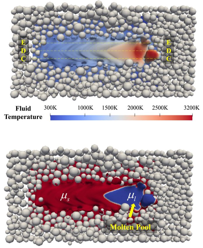
T. Yu and J. Zhao                                      Computer Methods in Applied Mechanics and Engineering 377 (2021) 113707

Table 2
Summary of major players on computational modeling of SLM.
 Primary institution                Method and         Ambient       Laser    Powder     Multiple    Missing crucial
                                    software           gas           model    layering   layers      phenomena
 Ohio State University              CFDb               ✔             IIIa     III        ✔           No metal vapor and
 (2009–2016 [63–68])                Flow-3D                                                          powder motion
 University of Erlangen–Nuremberg   CFD                ×             I        ×          ×           No metal vapor and
 (2010–2014 [69–73])                OpenFOAM                                                         powder motion
 University of Erlangen–Nuremberg   LBM                ×             III      III        ✔           No radiation, Marangoni
 (2011–2018 [69–74,74–88])          waLBerla                                                         term, metal vapor and
                                                                                                     powder motion
 ESI Software Germany GmbH          CFD             ✔                III      II         ×           No metal vapor and
 (2012–2019 [89–97])                ESI_ACE+                                                         powder motion
 UC Berkeley                        DEM & Continuum ×                I        II         ×           Simplified metal vapor,
 (2013–2019 [55–61])                method                                                           and no recoil pressure and
                                                                                                     Marangoni term
 Lawrence Livermore National        CFD                ×             I        III        ×           Simplified powder motion,
 Laboratory                         ALE3D                                                            and no mushy zone and
 (2014–2019 [12,47,98–106])                                                                          metal vapor
 University of Birmingham           CFD                ×             III      III        ×           No powder motion
 (2015–2018 [29,107–110])           OpenFOAM
 UC Berkeley                        SPH                ×             I        III        ×           No metal vapor and
 (2018 [17])                                                                                         powder motion.
 Peking University                  CFD                ✔             III      III        ✔           No recoil pressure, metal
 (2018 [52])                        OpenFOAM                                                         vapor and powder motion
 Nanyang Technological University   CFD                ✔             II       III        ×           No metal vapor and
 (2018 [111])                       OpenFOAM                                                         powder motion
 Leibniz University of              OTM                ✔             I        III        ×           No metal vapor and
 Hannover                                                                                            powder motion.
 (2019 [62])
 Hong Kong University of Science    CFD&DEM            ✔             II       I          ✔           No metal vapor
 and Technology                     OpenFOAM
 (Present)                          LIGGGHTS
a Note:
     I, II, III represent complete, moderate, and simple, respectively.
b Terminologies: SPH: Smoothed Particle Hydrodynamics; OTM: Optimal Transportation Meshfree; CFD: Computational Fluid Dynamics;
DEM: Discrete Element Method; LBM: Lattice Boltzmann Method.

will be demonstrated, the proposed approach is capable of considering key physical features in SLM, such as the
laser penetration, recoil pressure, Marangoni’s flow, and Darcy’s effects, and the effects of laser power, laser energy
distribution and hatch distance, as observed in experiments. It also expediates the simulation of repeated powder
layering process featured by complicated interactions among the roller, the standby powders, and the previously
melted layers, with full capability of integrated evaluation of the mechanical performance of final printed parts.

2. Methodology: A coupled CFD-DEM approach for SLM
   A coupled CFD–DEM approach is employed to simulate both the layering process and the melting process in a
typical powder-based selective laser melting in this study. Two physical flow processes in the SLM of powders are
broadly distinguished and treated separately, namely, the granular particle flow in an ambient gas over the solidified
molten layer during the powder layering process and the multiphase thermal-fluid flow and thermal-induced phase
changes during the melting process. The particle flow in an ambient gas and over a solidified molten layer during the
layering process is simulated using an unresolved CFD–DEM by virtue of its high computational efficiency, whereas
the multiphase thermal-fluid flow and thermal-induced phase changes during the melting process are tackled by a
semi-coupled resolved CFD–DEM for higher resolution and better accuracy. The combination of the two approaches
enables us to simulate the entire SLM process to obtain an accurate thermal field for both the particles and fluids
and to capture crucial physical processes in SLM, including the buoyancy force, Darcy’s effects, surface tension,
Marangoni’s flow, and recoil pressure [113]. The following presents the formulations and solution procedures of
the proposed methods.
                                                                 3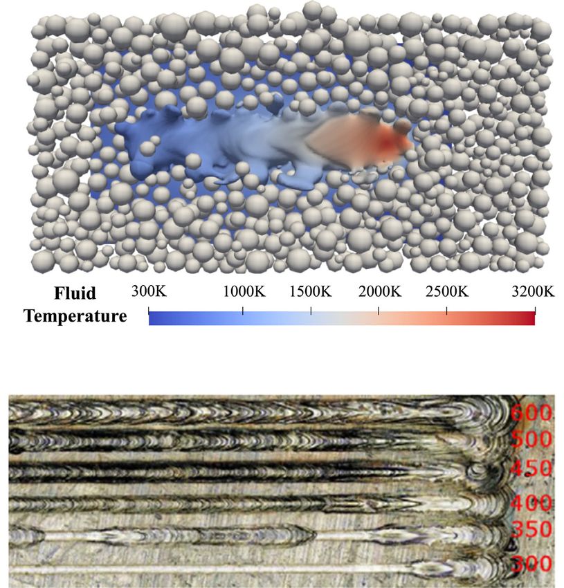
T. Yu and J. Zhao                                    Computer Methods in Applied Mechanics and Engineering 377 (2021) 113707

2.1. Unresolved coupled CFD-DEM for simulation of powder layering

    An unresolved coupled CFD and DEM is proposed to simulate a typical powder layering process for preparation
of laser melting. As a conventional coupling approach between CFD and DEM, the unresolved coupling formulation
is based on exchange of empirical estimation of interaction forces, such as the drag force [114], between the CFD
and DEM solutions for the fluid and particle phases, respectively. The approach typically adopts a CFD grid size
at least three times larger than the particle diameter in the DEM [52] to ensure reasonable accuracy and numerical
stability. There may be multiple powder particles resting in one CFD cell, such that the flow behavior among the
particles cannot be fully resolved but can only be estimated averagely over the cell.
    For a typical powder layering process, the primary interest is to establish a mechanically stable layer of granular
powders for preparation of the subsequent laser melting, whereas the air flow may be less important. Hence the
unresolved coupled CFD–DEM is a suitable choice. Indeed, we elect to solve the layering process by the unresolved
CFD–DEM specifically for a two-fold consideration. (1) It is assumed that the underlying molten track has been
solidified during the layering process where the particles will only collide with the solidified metal layer rather
than the molten flow, e.g., the interaction between them can be simplified as a particle–wall interaction. (2) When
the laser beam is withdrawn, the temperature of the molten track may drop to the room temperature quickly,
which will not further affect the particle motion and could be ignored in the unresolved CFD–DEM. Therefore, the
unresolved CFD–DEM is considered sufficiently accurate to solve the motion of the powder flow while maintaining
great computational efficiency. Note that the following formulation has been presented sufficiently general to allow
possible future extensions, e.g., to consider powder grains interacting with a molten track remaining in a fluid state.
    In this method, it is assumed the motion of each granular powder particle is governed by the following linear
and angular momentum equations and will be resolved by DEM:
       ⎧ dvp         ∑           ∑
       ⎨m p dt =
       ⎪                  Fp−p +     Fp−w + m p g + Ff
                    dωp     ∑         ∑                                                                               (1)
       ⎪
       ⎩         Ip       =      Mt +    Mr
                     dt
where m p and I p denote respectively the mass and rotational inertia of Particle p. g is the gravitational acceleration.
F p−p and F p−w are the particle–particle interaction force and particle–wall interaction force [115,116], respectively.
M t and M r are the torque from tangential force and rolling friction toque, respectively [117]. Ff is the particle–
fluid interaction force [118] including both drag force Fd and buoyancy force Fb for a general case. The drag force
exerted on the particle by its surrounding fluids which is considered as the dominant interaction force between
powder particles and surrounding fluid. Other interaction forces, such as inertial force, may be important depending
on the specific applications [119] but will be neglected in this study.
    The drag force Fd is calculated according to the following Hill–Koch formulation [120] and the buoyancy force
Fb is derived from the average density based expression [121]:
       ⎧        Vp β (         )
       ⎨Fd =           uf − vp
                 εp
                                                                                                                      (2)
              Fb = ρf Vp g
       ⎩

where Vp is the volume of the particle. ρf and uf are the density and velocity of the fluid, respectively. εp is the
particle void fraction in one cubic cell, and β denotes an empirical coefficient related to εp and the Reynolds
number [122].
   In the unresolved coupled CFD–DEM, the CFD will solve the following locally average Navier–Stokes equation
over each fluid cell [118]:
                            ∂ (
                                εp ρf + ∇ · εp ρf uf = 0
      ⎧                              )     (        )
                            ∂t
      ⎨
      ⎩ ∂ εp ρf uf + ∇ · εp ρf uf uf − εp ∇ (µ∇uf ) = −∇ p − fp + εp ρf g
            (      )       (          )                                                                                 (3)
         ∂t
where µ is the fluid viscosity and p is the fluid pressure. fp is the interaction force the particles inside the cell exert
on the fluid, which can be written as:
                 p
             nj
             ∑                      (Fd + Fb )i
      fp =           D(ri − r j )                                                                                       (4)
             i=1
                                        Vj
                                                            4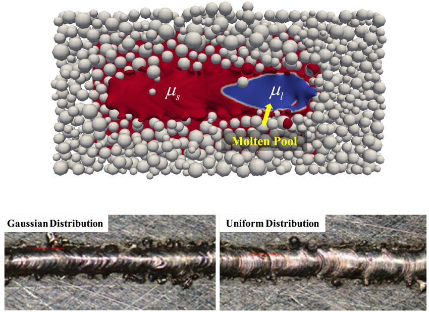
T. Yu and J. Zhao                                    Computer Methods in Applied Mechanics and Engineering 377 (2021) 113707

         p
where n j is the total number of particles in cell j. D(r i − r j ) is a distribution function [122] of the position vector
of the particles r i and the cell center r j . V j is the cell volume of cell j.
   The unresolved coupled CFD–DEM follows the following general solution procedure [118]:

(1) Set the initial and boundary conditions for the CFD and the DEM solvers.
(2) Evaluate the velocity field up of the fluid and pressure field p solving the Navier–Stokes equation without the
    source term f p , neglecting the physical existence of particles.
(3) Calculate the drag force exerted to a particle according to the evaluated uf and p and solve particle movements
    in Eq. (1) by DEM.
(4) Evaluate the source term f p based on the DEM solution such as the positions and velocities of particles and
    solve the Navier–Stokes equation (3) to provide updated velocity and pressure field.
(5) Proceed to next time step and repeat steps (3) and (4).

2.2. Semi-coupled resolved CFD-DEM for the melting process

    The melting of granular powder layer subjected to heating of a moving laser beam involves complicated
multi-phase, multi-physics processes featured by thermal transfer and thermal-induced phase transformation, and
solid–fluid–air interactions during their respective motions. Specifically, the heating of high-energy laser beam may
generate high temperature gradients within the powder grains that lead to full (in mid track) or partial (sidetrack)
melting of powders within the beam region. Driven by both Marangoni effect and recoil force (to be explained
later), the molten grains may flow viscously in preferential directions, push the motion of surrounding powders,
and form complex surface and inhomogeneous thermal fields during the gradual cooling process.
    To address the aforementioned challenges in simulating the melting process, a semi-coupled resolved CFD–
DEM method is proposed in this study. Specifically, the fully resolved coupled CFD–DEM based on the Immersed
Boundary (IB) method will be employed to resolve the velocity and pressure fields of the molten flow and the driven
motion of powder grains, whereas a dual-phase CFD is used to solve the thermal field including both fluid and solid
grains for the entire domain. The IB method is developed as the CFD solver in the fully resolved CFD–DEM here
to simulate the fluid flow around each solid particle. It requires a much smaller grid size that is at least smaller
than one eighth of the particle diameter [123], providing an accurate prediction of the drag force based on the
approach published by Shirgaonkar et al. [112] and hence more accurate flow behavior. Similar to the unresolved
coupled CFD–DEM, the fully resolved approach solves the fluids and particles separately at first. It then considers
the fluid–particle interactions by adding a force term derived from the presence of the solid particles that occupy
their real physical space to the Navier–Stokes equations to perform a correction for the velocity field of the fluid for
the solution [124]. However, a direct consideration of thermal transfer between the fluid and grain phases by CFD
and DEM may incur inaccurate thermal field, due mainly to the limitation that one DEM particle can only have
one single temperature, unless exceedingly complicated and costly treatments for each particle is made (e.g., by
refining each particle to small elements [125]). In avoiding these technical difficulties, a multi-phase CFD approach
is employed to solve the thermal field in this study. A fictious CFD domain occupied by the actual position of
particles is created as one phase and the actual molten flow as another. In so doing, the heat transfers between
the actual fluids and the fictitious particle domain can be resolved, with full respect of the temperature gradient
within each individual solid particle. Consequently, both partial melting and full melting of powder grains can be
simulated with the obtained high-resolution thermal field for all phases. For example, if in one metallic particle,
the temperature of some of its CFD cells is higher than the solidus temperature, these cells of the particle will be
deleted from the DEM domain and be replaced by high viscous fluids with the same initial shape in the CFD. As
such, partial melting can be modeled. Consequently, the combination of the fully resolved coupled CFD–DEM and
the multi-phase CFD is termed herein as the semi-coupled resolved CFD–DEM which enables us to exploit both
the advantages of CFD and DEM to simulate the melting process appropriately.
    In the semi-coupled resolved CFD–DEM, the particle–fluid interaction force exerted on each particle of the DEM
solver is computed according to the following expression proposed by Shirgaonkar et al. [112],
             ∑(
                  −∇ p + µρf ∇ 2 uf j · V j
                                   )
       Ff =                                                                                                          (5)
             j∈Th
                                                            5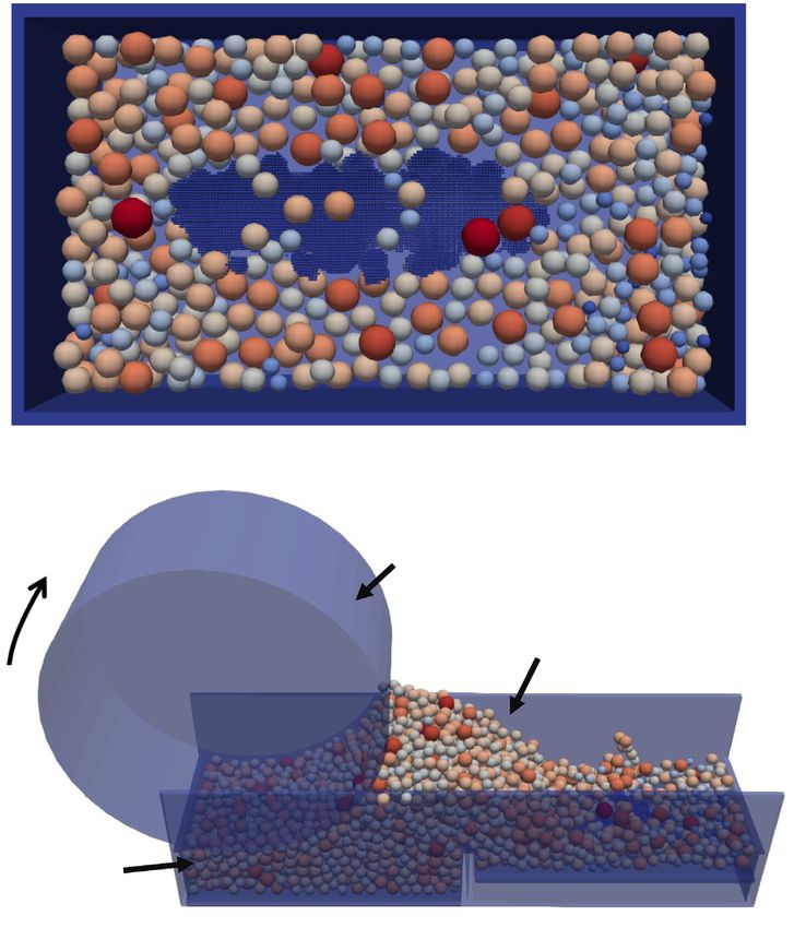
T. Yu and J. Zhao                                   Computer Methods in Applied Mechanics and Engineering 377 (2021) 113707

where p is the fluid pressure, uf is the velocity of the fluids, V j is the volume of cell j, and Th is the set of all
particle-covered cells.
    The multiphase flow has commonly been solved by the volume of fluid (VOF) method using volume fraction αi
to represent the co-existence of different phases in the domain. However, VOF can only obtain a smeared interphase
between different phases which requires a specific, complicated scheme to capture the sharp interface. For example,
the default scheme in OpenFOAM, MULES, employs a compressive flux term added into the advection equation
to compress the interface. In this study, a relatively new scheme called iso-Advector [126] is used to obtain the
complicated surface morphology of the melt flow featured with ripples, pores, denudation and balling effect in SLM.
In this scheme, isosurfaces are first reconstructed for the cells containing the interface to compute accurate surface
flux, the integral of which is then used to obtain the volume fraction field for next time step. A bounding procedure
is further applied to limit the values of volume fraction within specified range, which leads to the final interface.
Various classical validation tests [127,128] have demonstrated that the iso-Advector scheme offers more accurate
predictions on the interface between two phases than the MULES scheme.
    To facilitate the following presentation, we denote the volume fractions of the melt flow and the ambient gas in
a fluid cell for the fluid phase as α1 and α2 , respectively. Their relationship and the corresponding average density
ρ and equivalent viscosity µ [108] over the entire domain could be written as
            α1 + α2 = 1
       ⎧
       ⎪
       ⎪
       ⎨
         ρ = α1 ρ1 + α2 ρ2                                                                                         (6)
       ⎪
         µ = α1 µ1 + α2 µ2
       ⎪
       ⎩

Notably, these two physical parameters in Eq. (6) can be only used in the momentum equation if the semi-coupled
resolved CFD–DEM is employed. The presence of solid particles represented by a separate solid fraction εp should
also be considered when solving the thermal field. For certain cell under consideration, a solid fraction εp of 0
and 1 indicates respectively that this cell is inside or outside the DEM particle. Consideration of εp leads to the
following revised expressions for the density ρT , dynamic viscosity µT , thermal conductivity k, and heat capacity
C to be used in the temperature equation
           ρT = (α1 + 1 − εp )ρ1 + (α2 − 1 + εp )ρ2
      ⎧
      ⎪
      ⎪
      ⎪
      ⎨ µT = (α1 + 1 − εp )µ1 + (α2 − 1 + εp )µ2
      ⎪
      ⎪
      ⎪
                           ρ1                      ρ2                                                           (7)
        C = (α1 + 1 − εp ) C1 + (α2 − 1 + εp ) C2
                           ρ                       ρ
      ⎪
      ⎪
      ⎪
      ⎪
      ⎪
            k = (α1 + 1 − εp )k1 + (α2 − 1 + εp )k2
      ⎪
      ⎩

where the subscripts denote different phases.
   The flow dynamics of the fluid phase during both the layering and melting processes is assumed to be governed
by the Navier–Stokes equation. However, the momentum equation to be solved by the semi-coupled resolved
CFD–DEM presents the following form,
       ∂
         (ρf uf ) + ∇ · (ρf uf ⊗ uf ) = −∇ p + ∇ · (µ · (∇uf ))
      ∂t
                                                (α1 − αm )2                       2ρ
                                          −K c 3            uf + c · σ · |∇α1 |         n
                                                  αm + Ck                       ρ + ρ2
                                                         (                 ) 1                                        (8)
                                                                  T − TLV              2ρ
                                          +0.54 p0 exp L v · M                |∇α1 |         n
                                                                   RT TLV            ρ1 + ρ2
                                             dσ                                2ρ
                                          +      (∇T − n(n · ∇T )) |∇α1 |
                                             dT                            ρ1 + ρ2
where p is the fluid pressure, K c is the permeability coefficient, Ck is a constant to avoid division by zero, αm
is the volume
           [      fraction
                      (     of( the molten  ))]metal which can be approximated using a Gaussian error function [52],
αm = α21 1 + erf T −T    4
                            s
                               T  −  Tl +Ts
                                        2
                                                , Tl is the liquidus temperature, Ts is the solidus temperature, c is the
                      l
curvature of the fluid–gas interface, c = −∇ · n, n is the unit normal vector at the interface, n = ∇α1 / |∇α1 |, σ is
the coefficient of surface tension, L v is the latent heat of vaporization, M is the molar mass, T is the temperature,
TLV is the boiling temperature, R is the universal gas constant. |∇α1 | is an interface term to transform a surface
                                                           6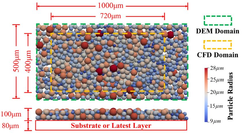
T. Yu and J. Zhao                                   Computer Methods in Applied Mechanics and Engineering 377 (2021) 113707

force per unit area into a volumetric surface force [111,129,130]. 2ρ/(ρ1 +ρ2 ) is a sharp surface force term to smear
out between two phases [108,131]. dσ/dT represents the change of surface tension coefficient with the temperature
and it is considered as a material constant in this work. The following equation is employed for surface tension
based on the surface tension coefficient of the metal at liquidus temperature σl
                 σl
           ⎧            [         (         (            ))]
                                       4         Tl + Ts
                          1 + erf             T−
           ⎪
                                                                 T ≤ Tl
           ⎪
           ⎨
      σ = 1 + erf2                  Tl − Ts         2                                                              (9)
                                       ∂σ                        T > Tl
                                  σl +
           ⎪
           ⎪                               T
                                       ∂T
           ⎩

   The last four terms on the RHS of the momentum equation in Eq. (8) represent the Darcy’s effects, surface
tension, recoil pressure and Marangoni’s flow, respectively. During the laser melting process, those partially melted
powders are considered as a mushy region with energy dissipation, which is described by the Darcy’s term [132,133].
When the temperature of the metal surface in the melt pool reaches the boiling temperature, evaporation will occur,
which results in a recoil pressure on the metal surface, commonly observed as the keyhole phenomena [111]. The
Marangoni’s flow shows an effect of difference in surface tension due to the temperature gradient in the melt pool
and its direction is parallel to the tangential direction of the melt flow surface [63]. These terms are essential to
simulate the evolution of various defects and reveal its mechanism.
   The melt flow and ambient gas in this simulation are assumed to be incompressible and their continuity equation
can be written as:
      ∇ · uf = 0                                                                                                      (10)
The temperature equation of the melting process is derived from the energy conservation, given by [108]
      ∂
         (CρT T ) + ∇ · (CρT uf T ) = Sl + ∇ · ∇(kT ) + µT (∇uf + uf ∇) : ∇uf
      ∂t
                                             ∂
                                          [                               ]
                                    − Lf        (ρT αm ) + ∇ · (ρT uf αm )
                                             ∂t
                                                                    2CρT
                                    − h c (T − Tref ) ⏐∇α ′ ⏐
                                                      ⏐      ⏐
                                                               (C1 ρ1 + C2 ρ2 )                                       (11)
                                                                      2CρT
                                    − σsb T 4 − Tref
                                           (           ) ⏐ ′⏐
                                                     4 ⏐
                                                          ∇α ⏐
                                                                 (C1 ρ1 + C2 ρ2 )
                                                                  (                )
                                              L v · M · p0                 T − TLV ⏐⏐ ′ ⏐⏐      2CρT
                                    − 0.82                    exp L v · M            ∇α
                                             (2π M RT )  0.5                RT TLV         (C1 ρ1 + C2 ρ2 )
where Sl is the laser input, α ′ = (α1 + 1 − εp ), L f is the latent heat of fusion, h c is the convective heat transfer
coefficient, Tref is the reference temperature, and σsb is the Stefan–Boltzmann constant. 2CρT /(C1 ρ1 + C2 ρ2 )
represents a sharp surface force term to smear out between two phases [108,131].
   The last six terms [52] in Eq. (11) represent the heat transfer due to conduction, dissipation, fusion, convection,
radiation, and evaporation. The laser source term Sl can be written as
      ⎧         fl
      ⎪
      ⎪  Sl =       Q l,S
      ⎪
      ⎪
      ⎪        ∆L
      ⎨ f l = α e 1 − e−γ z2
                ′
      ⎪
      ⎪           ( −γ z        )
                                                ⎡                                       ⎤
                                                                                                                    (12)
                                                ⎢ −2 (x − X l (t)) + (y − Yl (t)) ⎥
                                                                    2               2
                                                       [                              ]
      ⎪                      2P
         Q l,S = (                     ]2 ) exp ⎣
      ⎪
      ⎪
      ⎪                                                         [            ]2         ⎦
                                                          R 2 + λ (z − z )
      ⎪                    [
                  π R 2 + λ (z − z )
      ⎪
      ⎪
      ⎩               0     π R0      f                    0     π R0       f

where f l is the laser absorption coefficient based on the general Beer–Lambert form [134], which reflects an
exponential decay through the powder bed [135,136]. z 1 and z 2 are the depths from top to bottom side of the
cell under consideration in the powder layer, γ1 is the attenuation coefficient, P is the laser power, R0 is the laser
beam radius, z f is the z-coordinate of the lens focus, λ is the wave length of the laser, (x, y, z) is the coordinate of
the cell, and (X l (t) , Yl (t)) represents the center of the scanning path in the x–y plane.
   There have been various models proposed for calculating the absorption coefficient [52,108,131], but they rarely
consider the reflection and transmission of the laser. In this study, the penetration of the laser into powder layers
is considered, and the absorption model is further divided into two parts depending on whether the metal powders
                                                           7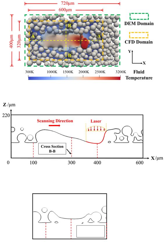
T. Yu and J. Zhao                                   Computer Methods in Applied Mechanics and Engineering 377 (2021) 113707

are fully melted. Experimental results [135] show that the penetration of laser beam into the powder layer is only
active prior to complete melting, after which the absorption will be confined to the surface of highly reflective
molten pool, as the attenuation coefficients of powders are much (e.g. four orders of magnitude) lower than for
bulk metal [137], e.g., iron and copper.
   If metallic powders are not melted, the initial attenuation coefficient γ1 in the absorption coefficient is determined
based on the experiment given by McVey [135]. When metallic powders begin to melt, the molten flow can be easily
heated over the boiling point [98], such that it is assumed that the surface of molten pool will absorb most of the
laser energy if the liquidus metal begins to evaporate. Existing absorption coefficient models [52,108,131] have
assumed only the upper two or three cell layers (interface) of the metal phase absorb the laser energy. In this work,
the upper four( cell layers of) the metal is assumed to absorb most (99%) of the laser energy when reaching the full
melting (i.e., 1 − e−γ2 ·4∆L = 0.99), such that the value of γ2 can be readily obtained. The attenuation coefficient
between these two conditions is approximated using a Gaussian error function,
                 γ2 − γ1
                          [         (           (               ))]
                                          4            TLV + Tl
      γ = γ1 +              1 + erf               T−                                                                 (13)
                     2                TLV − Tl            2
   The temperature field will be updated after solving Eq. (11). If the temperature of one cell in one particle is
higher than the liquidus temperature, this particle will be deleted in the DEM and replaced by spherical fluid cell
with a high solidus viscosity µs in the CFD. The solidus viscosity will decrease to liquidus viscosity µl when the
temperature reaches the liquidus point. Among studies [52,131,138] that approximate the viscosity transition from
the solidus temperature to liquidus temperature, the one proposed by Wang [52] provides an upper and lower limits
for the viscosity
                   [                (                     )]
              1            4                ln Tl + ln Ts
      ln µ = erfc                  · ln T −                  · (ln µs − ln µl ) + ln µl                       (14)
              2      ln Tl − ln Ts                2
where µs and µl are the viscosities at solidus temperature and liquidus temperature, erfc is the complementary
Gaussian error function.

2.3. Solution procedure for semi-coupled resolved CFD-DEM

   The proposed semi-coupled resolved CFD–DEM approach for SLM has been implemented in two open source
codes OpenFoam and LIGGGHTS with the help of a coupling engine CFDEM [139,140]. In the coupling, the IB
method is combined with the Pressure Implicit with Splitting of Operators (PISO), a standard pressure correction
approach for coupling velocity and pressure in CFD simulation [141]. The PISO algorithm consists of one predictor
step, where the pressure at the latest timestep is used to calculate the intermediate velocity, and of further corrector
steps, where the intermediate and final velocity and pressure fields are obtained iteratively [142]. In the PISO
Immersed Boundary (PISO-IB) scheme, the IB method is implemented into the standard PISO scheme to iterate
over the continuous forcing term added to the momentum equation that drives the motion of the immersed body.
Validation of the scheme can be found from various early test cases [143]. The PISO-IB scheme employed here is
based on the one modified by Hager [144].
   The following summarizes the complete solution procedure for the proposed semi-coupled resolved CFD–DEM
in conjunction with the PISO-IB scheme:

(1) Initialize CFD and DEM domains for the temperature field, pressure field, the velocity field of fluids and the
    velocity, position of powder particles;
(2) Calculate the drag force acting on the particles in Eq. (5) and update the particle motion using the Newton’s
    Second Law of Motion with a particle collision model in Eq. (1) [145], verify the temperature of each cell in
    the particle domain and remove a particle from the DEM if the temperature of any of its cells is higher than
    the solidus temperature and meets the partial melting criterion.
(3) Examine the change of void fraction field to identify whether the particle has been deleted and replace the
    deleted particles by fluid cells with identical temperature, and update all related parameters in Eq. (7) according
    to the new volume fraction field and temperature field, including density, heat capacity, thermal conductivity
    and viscosity.
                                                           8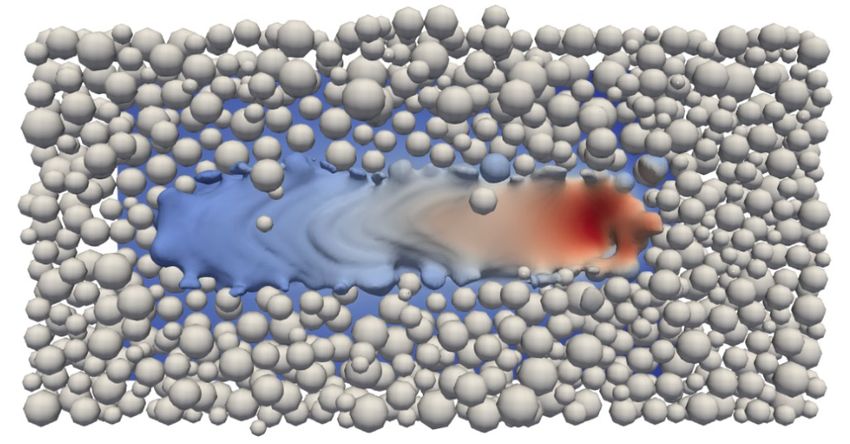
T. Yu and J. Zhao                                  Computer Methods in Applied Mechanics and Engineering 377 (2021) 113707

 (4) Calculate the laser source coefficient in Eqs. (12) and (13) based on the position of particles and fluids and
     the temperature field and update the temperature field based on the temperature equation (11) in CFD that
     considers the laser source, three heat transfer terms including conduction, convection and radiation, and the
     enthalpy change due to fusion and evaporation.
 (5) Calculate the volume fraction of the metal and protective gas and reconstruct the surface of melt flow using the
     iso-Advector scheme, a sharp VOF-based interface capturing method, and then update all related parameters in
     Eq. (7) according to the new volume fraction field and temperature field.
 (6) Update the velocity field uf and pressure field p0 by solving the Navier–Stokes equation (8) over the whole
     domain, where the existence of particles is neglected but the buoyancy force, Darcy’s effects, surface tension,
     Marangoni’s flow, and recoil pressure are considered instead.
 (7) Calculate the drag force exerted on the particles based on the evaluation of uf and p0 in Eq. (5) and solve DEM
     for particle motion in Eq. (1).
 (8) Correct the old velocity field into the new velocity field u in two steps: (a) Calculate u0 by correcting the old
     velocity field in the particle domain (u0 = vp ) and the interface (u0 = (1 − εp )(vp + ωp × r) and εp is the
     void fraction, r is the position vector of the particle). (b) Further correct the velocity field u0 according to
     u = u0 − ∇φ, where ∇ 2 · φ = ∇ · u0 to satisfy the mass conservation under the hypothesis of incompressibility,
     and then update the pressure p0 using p = p0 + ρ · ∇φ/∆t.
 (9) Go to step (6) to repeat the PISO loop until the residual error or the cycle number reaches the prescribed
     threshold.
(10) Go to step (1) to repeat the entire simulation until reaching the final time step.

 3. Simulation of SLM: Results and discussion
 3.1. Model setup and parameter selection

    This study takes the melting process of a typical titanium alloy Ti-6Al-4V powder as an example for the proposed
 numerical approach. Relevant physical parameters [131] adopted for the modeling are shown in Table 3.
    It is physically more realistic to use temperature-dependent thermal parameters [52] for the considered metallic
 powder. Following American Society for Metals (ASM) [146], the following temperature dependent density ρ1 , heat
 capacity C1 , and thermal conductivity k1 of Ti-6Al-4V alloy are adopted
                                                                   T < 1268K
        ⎧                         ⎧
        ⎪                         ⎨         4420
                   ρ        3
                                                                     < T < 1923K
        ⎪
        ⎪
        ⎪
        ⎪
        ⎪           1 (kg/m   ) =   4420 − 0.154(T  − 298)    1268K
                                   3920 − 0.680(T  − 1923)         T ≥ 1923K
        ⎪
        ⎪                         ⎩
        ⎪
        ⎪
                                                                      T < 1268K
        ⎪                         ⎧
        ⎪
        ⎪
        ⎪                         ⎨           411.5
               C1 (m2 /(s2 K)) = 411.5 + 0.2T + 5 × 10⁻⁷ T 2 1268K < T < 1923K
        ⎪
        ⎨
                                                                                                                (15)
                                               830                     T ≥ 1923K
                                  ⎩
        ⎪
        ⎪
                                                                          T < 1268K
        ⎪                        ⎧
                                               19.0
        ⎪
        ⎪
        ⎪                        ⎪
                                                                            < T < 1923K
        ⎪                        ⎪                            −6 2
                                  −0.797 + 0.0182T  −  2 × 10   T    1268K
        ⎪
        ⎪                        ⎨
          k1 (kg m/(s3 K)) =
        ⎪
                                                                            < T < 1973K
        ⎪
                                               33.4                  1923K
        ⎪
        ⎪
        ⎪
        ⎪                        ⎪
                                 ⎪
                                               34.6                       T ≥ 1973K
        ⎩                        ⎩

 The chosen viscosity at solidus temperature µs is crucial for the accuracy of simulation results. A high viscosity
 may help to ensure the movement of those fluids close to that of the solid powders and hence a much larger Deborah
 Number than 1 [147]. Experimental data [148] show that the viscosity µs of Ti-6Al-4V alloy is larger than 107.5
 Pa s at low strain rate (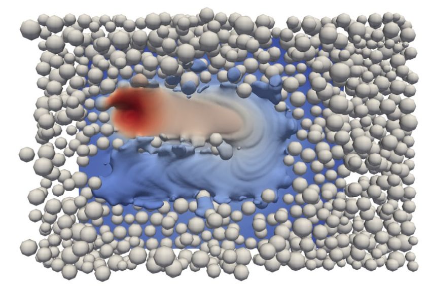
T. Yu and J. Zhao                                                  Computer Methods in Applied Mechanics and Engineering 377 (2021) 113707

Table 3
Physical parameters of the numerical model.
 Parameter                                       Value and units                Parameter                                   Value and units
 Liquidus temperature                       Tl = 1923 K                         Solidus temperature                         Ts = 1878 K
 Boiling temperature                        TLV = 3133 K                        Initial temperature                         T0 = 300 K
 Laser Diameter                             DL = 140 µm                         Laser velocity                              vL = 60 cm/s
 Atmospheric pressure                       p0 = 101 000 Pa                     Molar mass                                  M = 446.07 g/mol
 Viscosity of air                           µ2 = 1.5 × 10⁻⁵ m2 /s               Heat capacity of air                        C2 = 1164 m2 /s2 K
 Latent heat of fusion                      L f = 2.88 × 10⁵ m2 /s2             Air density                                 ρ2 = 1 kg/m3
 Latent heat of evaporation                 L V = 4.7 × 10⁶ m2 /s2              Viscosity of liquidTi-6Al-4V alloy          µl = 0.005 Pa s
 Initial attenuation coefficient            γ1 = 0.0144                         Surface tension coefficient at melt point   σl = 1.5 kg/s2
                                            ∂σ
 Change rate of surface tension coefficient      = −2.6 × 10⁻⁴ kg/(s2 K)        Convective heat transfer coefficient        h = 19 kg s3 K
                                            ∂T

              Table 4
              Model properties and computational domain of four cases.
                Type                                       Property                          CFD Domain            DEM Domain
                                                           5 µm–200 W − Gaussian             L = 600 µm            L = 720 µm
                Convergence study (Single track)           4 µm–200 W − Gaussian             W = 320 µm            W = 400 µm
                                                           3.5 µm–200 W − Gaussian           H = 220 µm            H = 300 µm
                                                           4 µm–300 W − Gaussian             L = 720 µm            L = 1000 µm
                Validation test (Single track)             4 µm–150 W − Gaussian             W = 400 µm            W = 500 µm
                                                           4 µm–200 W − Uniform              H = 220 µm            H = 300 µm
                                                           4 µm–200 W-Gaussian               L = 720 µm            L = 1000 µm
                Validation test (Multiple tracks)          Hatch distance = 1.25DL           W = 576 µm            W = 680 µm
                                                           4 µm–200 W-Gaussian               H = 220 µm            H = 300 µm
                                                           Hatch distance = DL               L = 720 µm            L = 1000 µm
                                                           4 µm–200 W-Gaussian               W = 512 µm            W = 620 µm
                                                           Hatch distance = 0.75DL           H = 220 µm            H = 300 µm
                                                                                             L = 640 µm            L = 900 µm
                Multi-layer model (Single track)           4 µm-200 W-Gaussian               W = 400 µm            W = 500 µm
                                                                                             H = 320 µm            H = 300 µm

around 36 µm, nine times of the length of grid size (4 µm) used in the CFD domain. Fig. 1(b) presents the
model setup for the subsequent convergence study, validation and multi-layer simulations. A smaller CFD domain
compared to that of the DEM is adopted to reduce the computational cost. Table 4 summarizes the model properties
used in the following simulations, including the grid size, laser beam and simulation domain. As for the naming
of laser beam indicated in the table, 4 µm-200 W-Gaussian means that the grid size is 4 µm and the laser energy
is 200 W with a Gaussian distribution. In addition to convergence and validation studies, we will also present a
multi-layer simulation where both the layering process and the melting process are modeled. During the layering
process, the standby powders are compressed within the work area by a roller a radius of 1000 µm and height of
500 µm to form a new layer preparing for melting.
   A substrate of 80 µm in thickness is considered and is overlaid by a powder bed 100 µm thick. The time step of
CFD is set to be 1 ×10⁻⁷ s, ten times of that for the DEM (1 ×10⁻⁸ s). The bottom boundary is set as a non-slip
wall and zero gradient for both temperature and pressure, and other boundaries are set as fixed value for pressure
and zero gradient for velocity and temperature.

3.2. Convergence study

    A convergence study is performed to determine a proper grid size for the validation model that offers balanced
efficiency and accuracy for the computation. Previous numerical experience on unresolved coupled CFD–DEM
studies indicates the accuracy of simulation results can be guaranteed if the particle size is 8 times larger than
the grid size [123]. With a mean diameter of powders of 36 µm, three cases of CFD grid sizes (5 µm, 4 µm and
3.5 µm) are considered. The top view of the simulation result for the case of grid size 4 µm is shown in Fig. 2(a),
                                                                          10
T. Yu and J. Zhao Computer Methods in Applied Mechanics and Engineering 377 (2021) 113707
Fig. 1. Model setup for coupled CFD–DEM simulation of SLM of Ti-6Al-4V alloy powder.
and the longitudinal section A–A at y = 160 µm and the cross section B–B at x = 300 µm are chosen, as shown
in Fig. 2(b) and (c).
Fig. 3 shows a comparison of the longitudinal and transverse cross section contours of the molten track with
different grid sizes where contours in black, red and blue represent grid size cases of 5 µm, 4 µm and 3.5 µm,
respectively. Particular attention is paid to the longitudinal section A–A of the molten track behind the laser spot
from x = 100 µm to x = 400 µm and the cross-section B–B ranges from y = 50 µm to y = 320 µm. Evidently,
similar contours are observed at the three cases of grid size. The maximum difference between the black and red
11T. Yu and J. Zhao Computer Methods in Applied Mechanics and Engineering 377 (2021) 113707
Fig. 2. Top view and cross section contours of the molten track with CFD grid size 4 µm.
12T. Yu and J. Zhao Computer Methods in Applied Mechanics and Engineering 377 (2021) 113707
Fig. 3. Cross section contours of the molten track with three grid sizes.
contours is about 4 µm, which only mildly changes the curvature of the molten track surface rather than the whole
structure.
Fig. 4 further shows the temperature profile of the same longitudinal section A–A contour, from x = 110 µm to
x = 400 µm in x direction. The black and red contours are well overlapped except in the region from x = 300 µm
to x = 375 µm due to the high temperature and difference in cross section B–B contours. Note that the absorption
coefficient is also related to the grid size. However, since the maximum temperature difference is only about 130
K, which is around 5% of the temperature at that point, the difference between the cross-section contours from x
= 150 µm to x = 200 µm does not result in an appreciable temperature difference due to the solidification. In the
rest of this paper, a grid size of 4 µm of CFD is adopted to balance the accuracy and efficiency.
3.3. Validation of model predictions against experimental data
The multiscale predictions of SLM based on the semi-coupled resolved CFD–DEM are further validated by
experimental data in this subsection. Specifically, three validation cases with varying laser power, laser energy
distribution, and hatch distance of multiple tracks are considered.
Fig. 5 shows the Marangoni driven ripples and piled track-heads captured by our multiscale approach in
comparison with observations from experiments [151]. Marangoni effect is typical flow instability observed in SLM,
caused by high fluid temperature gradient that induces changes in surface tension. As the surface tension decreases
with increasing temperature for Ti-6Al-4V alloy, the low temperature molten flow behind the laser spot has a higher
surface tension which drives the molten pool flowing back to form the ripples during quick solidification. In this
simulation, the scanning speed is 60 cm/s and three laser powers, 150 W, 200 W and 300 W, are tried. When
the laser power grows stronger, the ripples become larger in size and sharper, due primarily to larger molten pool
and higher temperature gradient caused. Increasing laser power may lead to initially dense but later sparser ripples.
When the laser power is low, the energy may not be sufficient to form ripples in some regions. However, if the laser
13T. Yu and J. Zhao Computer Methods in Applied Mechanics and Engineering 377 (2021) 113707
Fig. 4. Temperature profiles along longitudinal section A–A with different grid sizes.
power is adequately high, relatively larger molten pool, higher temperature gradient and recoil force may combine
to result in closer ripples, increased thickness, size and interval of final ripples. These phenomenon are consistent
with the experimental observations [151] shown in Fig. 5(d).
The distribution of laser energy during the melting process can also affect the formation of ripples and the
surface quality of molten track. Experimental results [34] have confirmed that the molten track formed by a uniform
distributed laser energy is more regular and flatter compared to a Gaussian distributed one. A comparison of the
numerical predictions by the Gaussian and uniform distribution types of laser energy is presented in Fig. 6 at a laser
power of 200 W. In the figure, the viscosity contour features a red subregion representing the solidus viscosity and
a blue one for the liquidus viscosity. The latter is also commonly called molten pool. A further comparison of the
molten pool with the ripples in Fig. 6(a) shows that the two are highly coincident with each other, confirming that
the ripples is indeed dominated by the molten pool. Since the Gaussian distribution of laser energy has its energy
concentrated at the laser center, it is reasonable to find that higher temperature gradient and sharper ripples are
observed as compared to the uniform laser energy distribution case.
The roughness of the molten track is one of the important indices for quality control of SLM. It is evaluated in
this study using a commonly used one-dimensional roughness parameter, the arithmetic average roughness Ra. Three
longitudinal sections (Fig. 6(a)) of the solidified molten track, at y = 150 µm (section C–C), y = 200 µm (section
D–D) and y = 250 µm (section E–E), respectively, are chosen to calculate the corresponding average thickness
dm and average roughness Ra (Fig. 7). The longitudinal section D–D refers to the center line of the molten track
wherein Ra is smaller when the laser power is 300 W which can provide sufficient energy to have the powders
fully melted. Pores may be generated at the bottom of the powder bed with a low laser energy, such as the case of
laser energy at 200 W. It should be noted that the two polylines in the case of Gaussian distribution laser energy
present a ‘V’ shape because the laser energy is primarily concentrated at the center of molten track, leading to less
energy and insufficient melting and thus a rough surface along the track edge. It can be concluded that the surface
of the molten track is flatter and smaller surface roughness when subjected to a uniform laser energy distribution.
By virtue of the coupled CFD–DEM formulation, the powder movement during the melting process can also be
captured, which has not been attempted by existing studies. Critical in driving the powder movement during the
melting process are the vapor recoil and the spatially varying absorptivity [152], which may cause localized fluid
flow and further interactions with surrounding powders [98]. The interactions between melt flow and surrounding
14T. Yu and J. Zhao Computer Methods in Applied Mechanics and Engineering 377 (2021) 113707
Fig. 5. Comparison of multiscale simulation of SLM with different laser power (a–c) with experimental observations (d).
particles and particle–particle collisions have been captured in our simulation. Fig. 8 shows a qualitative comparison
of experimental observations by high speed imaging [98] and our simulation results. In the figure, yellow arrow
trajectories represent powders swept away from the molten pool, whereas others indicate powders falling into the
molten pool. Note that vapor could serve as a dominant factor [98] not considered for the powder movement in this
study. It will be considered in a future work.
The hatch distance is a dominant factor in multi-track SLM, controlling the manufacturing efficiency and surface
quality. Fig. 9(a) shows experimental observations of the surface quality of multiple molten tracks [10,153,154] with
appreciable discontinuities and sticking particles along the step edges that all contribute to the increase of surface
15T. Yu and J. Zhao Computer Methods in Applied Mechanics and Engineering 377 (2021) 113707
Fig. 5. (continued).
roughness. Note that the discontinuities have been a result of the so-called ‘balling effect’ or ‘Plateau–Rayleigh
instability’ due to surface tension. This defect can be eliminated using the scanning strategy with overlapped scan
tracks, as shown in Fig. 9(b). For example, A 25% scan overlap can effectively remove the discontinuity at the
step edge [155], reaching a higher Vickers microhardness value of final samples. Our numerical approach can
faithfully reproduce the phenomenon and the remedy. As shown in Fig. 10, three multi-track numerical simulations
are performed with a hatch distance at 125%, 100% and 75% of the laser diameter, respectively. Evidently, when
the hatch distance is greater than the laser diameter, both sticking particles and discontinuity can be observed
(Fig. 10a). Reducing the hatch distance to the same size of laser diameter can help eliminate the sticking particles
but discontinuity due to balling effect can be still found (Fig. 10b). With a 25% overlapping, both defects can be
effectively reduced (Fig. 10c).
3.4. Simulation of multi-layer SLM
SLM is commonly based on a layered manufacturing process where a single layer of molten track is formed
from the metallic powders and is bonded to previous layers until the final object is completed [156], as illustrated
in Fig. 11. This section further demonstrates the capacity of our proposed method in modeling multi-layer SLM
process. The same set of model parameters as listed in Table 4 are used.
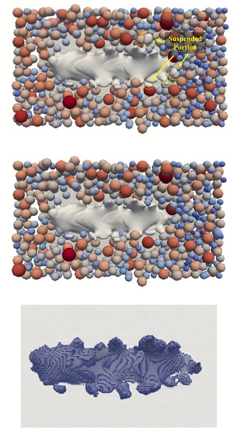
We follow four steps to model the preparation for the next powder layer after melting the former layer. (1)
Remove the suspended portion (Fig. 12(a)) of the molten track due to the extremely high viscosity and Darcy’s
16T. Yu and J. Zhao Computer Methods in Applied Mechanics and Engineering 377 (2021) 113707
Fig. 6. Comparison of simulation (a–c) and experiments (d) on the melting by different laser energy distributions.
effects (Fig. 12(b)) that may adversely affect the subsequent layering process. These suspended parts refer to the
spatters observed in experiments which would cause the denudation zone if left uncleared [98]. The unresolved
CFD–DEM with a large grid size (150 µm) as described in Section 2.1 is used in this step. (a) Replace the molten
track in the CFD by fixed particles with the same diameter as the grid size to ensure accurate transformation of
complex molten surfaces, as shown in Fig. 12(c). The replacement only applies to cells with a volume fraction1
larger than 0.5 where particles are in the center of cells. In doing so, the interaction between the powders and
the solidified metal can be simplified as the collision between particles in the DEM. (3) Perform DEM simulation
to bring all moving particles into an static equilibrium state (Fig. 12(d)), and use a roller to press and push the
standby particles from the left side to the work area in the fourth step (Fig. 12(d)), finishing the layering process.
(4) Apply laser beam and melt this new particle layer. The above four steps are repeated to simulate a multi-layer
SLM process to finish a design product.
Significant surface roughness along the edge of multi-layer molten tracks and apparent ripples are found in both
our simulation results and SEM images of experimental tests [157] (Fig. 13). The surface roughness is composed
of sticking powders, partially melted powders and discontinuities caused by balling effect [155]. It may affect the
surface quality and the mechanical properties of the final fabricated product. As shown in Section 3.3, a 25% overlap
between two neighboring tracks can help efficiently eliminate this defect. The overlapping strategy, however, may
17T. Yu and J. Zhao Computer Methods in Applied Mechanics and Engineering 377 (2021) 113707
Fig. 6. (continued).
Fig. 7. Simulation results of average height dm and average roughness Ra.
18T. Yu and J. Zhao Computer Methods in Applied Mechanics and Engineering 377 (2021) 113707
Fig. 8. Simulated powder movement during the melting process (a) in comparison with experiments (b).
not work for some special situations, such as the porous implant structure shown in Fig. 13(c), as the working area
may be limited in size to allow multiple tracks and significant overlapping and hence this defect may remain in the
product. Nevertheless, the proposed approach may serve as a robust analytical tool for systematic parametric study
in this case for design of optimal printing strategies.
4. Conclusions and outlooks
A semi-coupled resolved CFD–DEM approach has been proposed for solving a class of granular media problems
that involve thermal-induced phase changes and particle–fluid interactions. It has been validated by a typical
powder-based selective laser melting (SLM) process using titanium alloy Ti-6Al-4V. The influences of laser power,
laser energy distribution and hatch distance on the melting quality have been examined. It is demonstrated that
the proposed approach is capable of capturing key features and observations found in SLM experiments and its
predictions are consistent with existing data. An unresolved CFD–DEM has been further employed to simulate the
layering process for preparing the next powder layer after melting of one layer. A combination of the semi-coupled
resolved CFD–DEM for the melting process and the unresolved CFD–DEM for the layering process of next particle
layer offer a complete cycle of multi-layer simulation framework for powder-based SLM. Major conclusions drawn
from the study are summarized as follows:
19T. Yu and J. Zhao Computer Methods in Applied Mechanics and Engineering 377 (2021) 113707
Fig. 9. SEM images of multiple molten tracks observed in experiments (see [154]).
(a) The semi-coupled resolved CFD–DEM method features the employment of Immersed Boundary Method to
model the viscous fluids surrounding each solid particle in conjunction with a fictious CFD domain occupying
the actual position of particle. It expediates the modeling of heat transfers between the actual fluids and the
fictitious particles as a multiphase problem within the CFD, whereas the particle–fluid interactions can be treated
by the coupling between DEM and CFD.
(b) A unified coupled CFD–DEM framework combining the semi-coupled resolved CFD–DEM and the unresolved
CFD–DEM as described in the study can help effectively reproduce the entire SLM processes, including
resolving the motion of powders, dynamics of molten flow, and powder-flow interaction. This framework
provides a basic methodological tool for future optimization of powder based SLM over various factors, such
as the scanning strategy, initial temperature and deposition method.
(c) Three phases, including the ambient gas, solid metallic powders and molten flow can be fully built in this
melting process and rigorously modeled by the semi-coupled resolved CFD–DEM. Key to the success of the
proposed method is the integration of the iso-Advector method and the Immersed Boundary Method to resolve
accurate molten surfaces and particle–fluid interactions in conjunction with an absorption model to capture the
interactions between laser energy penetration and highly reflective molten pool that result in multiple phenomena
including the phase change, Marangoni effect, recoil force and Darcy’s effects. Simulation results with different
laser power, laser energy distribution and hatch distance demonstrate the proposed method can capture crucial
20You can also read