Simulation of non-radiative energy transfer in photosynthetic systems using a quantum computer
←
→
Page content transcription
If your browser does not render page correctly, please read the page content below
Simulation of non-radiative energy transfer in photosynthetic systems using a quantum computer
Simulation of non-radiative energy transfer in photosynthetic
systems using a quantum computer
José Diogo Guimarães1,2 , Carlos Tavares1,3 , Luís Soares Barbosa1,3,5 and Mikhail I.
Vasilevskiy2,4,5
arXiv:2009.01283v1 [quant-ph] 2 Sep 2020
1
Department of Informatics, University of Minho, Campus de Gualtar, Braga, Portugal
2
Department of Physics, University of Minho, Campus de Gualtar, Braga, Portugal
3
High-Assurance Software Laboratory, INESC TEC, Departament of Informatics, University of Minho, Campus
de Gualtar, Braga, Portugal
4
Centro de Física, Universidade do Minho, Campus de Gualtar, Braga, Portugal
5
International Iberian Nanotechnology Laboratory, Braga, Portugal
Abstract
Photosynthesis is an important and complex physical process in nature, whose comprehensive understanding would
have many relevant industrial applications, for instance in the field of energy production. In this paper we propose
a quantum algorithm for the simulation of the excitonic transport of energy, occurring in the first stage of the
process of photosynthesis. The algorithm takes in account the quantum and environmental effects (pure dephasing),
influencing the quantum transport. We performed quantum simulations of such phenomena, for a proof of concept
scenario, in an actual quantum computer the IBM Q, of 5 qubits. We validate the results with the Haken-Ströbl
model and discuss the influence of environmental parameters on the efficiency of the energy transport.
Introduction
Photosynthesis is a vital and pervasive complex physical process in nature, where the radiation of the Sun is cap-
tured by certain living beings, such as plants and bacteria, and transformed into the necessary carbohydrates needed
for their survival [29, 35]. From the physics and chemistry perspective, it is a complex process occurring through
several stages with several kinds of physical phenomena involved, namely, the light absorption, energy transport,
charge separation, photophosphorylation and carbon dioxide fixation [17]. The understanding of such phenomena
has greatly progressed in the the past 40 years with the physical characterization of the structure of many photosyn-
thetic complexes [7, 12, 48]. The comprehension of such processes would allow for many potential huge-impact
industrial breakthroughs in the field of energy, from the great efficiency improvement in energy capture of solar
panels [32] to the construction of artificial light-harvesting devices and solar fuels [20, 21, 45, 57].
The photosynthesis begins by the absorption of a photon. It occurs via excitation of a pigment molecule, which
acts as a light-harvesting antenna connected to the rest of the photosynthetic apparatus by protein molecules. Pho-
tosynthetic pigment-protein complexes transfer the absorbed sunlight energy, in the form of molecular electronic
excitation, to the reaction center, where charge separation initiates a series of biochemical processes [35]. This
work is focused on the first stage of photosynthesis, more precisely, on the transport of the absorbed radiation en-
ergy from the antenna to the reaction centre, which proceeds in the form of the so-called Excitonic Energy Transfer
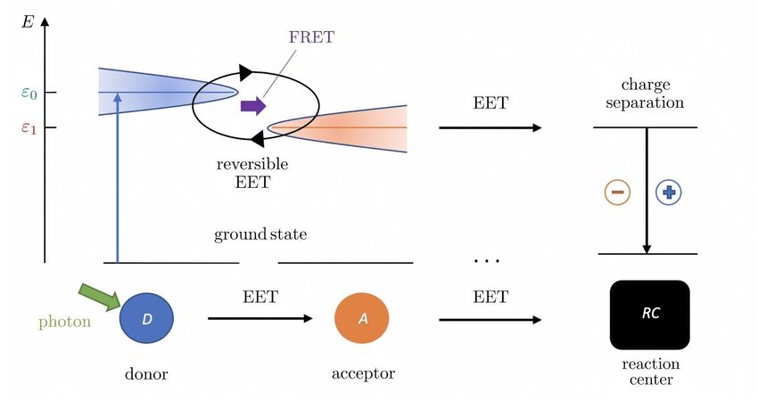
(EET), as schematically shown in Fig.1.
1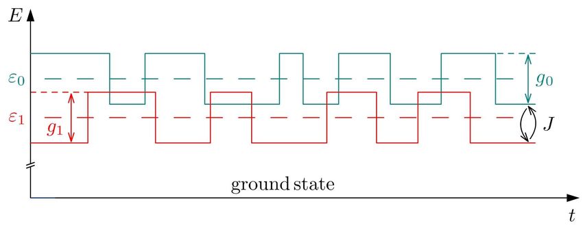
Simulation of non-radiative energy transfer in photosynthetic systems using a quantum computer

Figure 1: Schematics of the energy transfer process from light-harvesting antenna (the donor) through a chain
of acceptor molecules to the reaction center. The excited states of the participating molecules, denoted m , are
broadened and it allows for resonance energy transfer via irreversible Förster-type resonant process of exciton
transfer from donor to acceptor even if m 6= m+1 , which is denoted by the thick arrow labelled FRET. However,
if the coupling between the donor and the acceptor molecules is strong enough, the process becomes reversible and
the exciton can go to and through many times before it is transferred; this situation is labeled by "reversible EET"
and it does not require matching of the energy levels m and m+1 .

    This transport is known to be very efficient in photosynthesis, as is the whole process, with the overall quantum
efficiency of initiation of charge separation per absorbed photon up to 95% [35]. The absorbed photon creates
an exciton on the antenna molecule, which can eventually transfer it to other molecules. In this context, it is
called donor, while the others are called acceptors and the EET process can be described by the following reaction
equation:
                                                D ? + A → D + A? .                                                 (1)

     The physics of the mechanisms behind Eq. (1) will be discussed in the following section. Here we just notice
that EET is a complex process that can be irreversible (i.e. unidirectional) or reversible, i.e. coherent over some pe-
riod of time as evidenced by experimental observations of long-lived oscillatory features in the dynamical response
of several photosynthetic systems [14, 23, 30]. Moreover, it is strongly influenced by the environment. The donor-
acceptor pair is not isolated from the rest of the world and is an example of so called open systems [42]. It must be
treated as a subsystem of a larger system including a thermal bath. The properties of the latter are crucial because
it introduces relaxation and dephasing into the system directly involved in the EET and, therefore, influences the
efficiency of the energy transport.
     Open quantum systems cannot be described by a wave function because one does not have enough information
to specify it, only a (less detailed) description in terms of a density matrix is possible, which represents a statistical
mixture of states, or a mixed state (see Supplementary information A.1). The dynamics of such a system can
be determined by solving an equation of motion for the density matrix. Such equations of motion are called
quantum master equations. Finding exact solutions to the master equations is extremely difficult but there is a wide
range of theoretical approaches and techniques available to make their mathematical simplification and numerical
simulations. These approaches can be divided into several groups according to the regime under study, characterized
by the coupling strength between the bath and the system, and the existence of memory effects in the bath (i.e.
whether the system can be considered as Markovian or not). Broadly speaking, for the weak-coupling Markovian
regimes, perturbative approaches are applicable, such as the Bloch-Redfield and Lindblad master equations [26,

                                                            2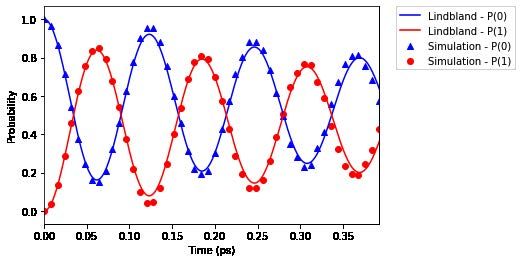
Simulation of non-radiative energy transfer in photosynthetic systems using a quantum computer

35], which can be extended to medium coupling strengths and non-Markovian regimes by including higher-order
system-bath interaction terms [25, 44]. For the latter regime, there are also non-perturbative techniques based on the
use of path integrals to dissipative systems [16], which can be used to create sets of solvable systems of hierarchical
equations, the so-called hierarchical equations of motion (HEOM) [24, 50, 51]. Open quantum systems that do not
have the Markovian property, for example, because of a too small size of the bath effectively coupled to the system,
which keeps memory of the past, are much more difficult for theoretical description because the dynamics equation
is non-local in time.
    However, even within the Markov approximation, the calculations quickly become computationally intractable
for realistic photosynthetic systems and environment models. The computational cost of simulating a photosyn-
thetic complex consisting of N molecules with a theoretical tool such as the HEOM grows exponentially with N . A
possible computational solution has been arising to bypass this type of problems is the use of quantum simulation,
where it is expected to obtain large performance increases in terms of space, as the number of qubits’ growth is just
polynomial, and in terms of time, where an exponential gain is expected.
    The use of quantum mechanics to make calculations about quantum mechanics, promising great computational
advantages was firstly proposed by R. Feynman [15, 33]. The field of quantum simulation is under a fast paced
and intense development, finding already application across all fields of physics and using many different physical
implementations [19]. Closer to the present work, there are works on quantum transport [34, 47] and on the
quantum simulation of dissipative systems [13]. Particularly on the quantum simulation of photosynthesis, we
would like to highlight Refs. [37, 41, 52], using superconducting qubits, and [54] employing a Nuclear Magnetic
Resonance (NMR) simulator [58]. The latter is of particular relevance to the work carried out here as it was
dedicated to the quantum simulation of the energy transport with environmental actions, where the environment
effect is simulated naturally by an appropriate filtering of environmental noise [49], within the NMR system. In this
case, the implementation is specific for the EET (i.e. non-universal), and the model Hamiltonian was extracted from
spectroscopic data for a photosynthetic system [2]. We are simulating the same Hamiltonian as in Ref. [54] and
starting from the same assumptions, however, the simulation algorithm is completely different since we conceived
a digital quantum simulation designed to run in a universal quantum computer, the commercially available IBM Q
of 5 qubits [11]. Our implementation contains a quantum part, aimed at simulating the unitary part of the system’s
evolution, and a classical part that simulates the stochastic interaction with the environment, the latter only being
able to mimic pure dephasing environmental effects.

The physics of the energy transport in photosynthesis
Förster and Redfield approaches
The molecules of the light-harvesting complexes usually are not electronically coupled to each other and charge
transfer via electron tunneling is improbable. Hence, energy transfer can occur between them through electromag-
netic interaction, without net charge transport because the whole (neutral) exciton is transferred. Such processes
are known to take place between molecules [3] or artificial nanostructures such as quantum dots [46] if appropriate
conditions are met, which were first formulated by T. Förster [18]:
    (i) The distance between the donor and acceptor molecules must be sufficiently small because the transfer
probability decreases quickly with the distance between them (R), usually as R−6 ;
    (ii) There must be a resonance between the excited states of the donor and acceptor molecules;1
    (iii) An increase of the refractive index of the surrounding medium decreases the transfer rate.
    Förster’s approach is based on the second-order perturbation theory (the so called "Fermi’s Golden Rule"),
where the perturbation operator is the electromagnetic interaction between two transient dipoles corresponding
to allowed optical transitions in the donor and acceptor molecule, respectively. It originated the term "Förster
   1 "Resonance"   here means that the energy spectra of the two molecules, broadened because of a number of natural reasons, overlap - see
Fig.1

                                                                     3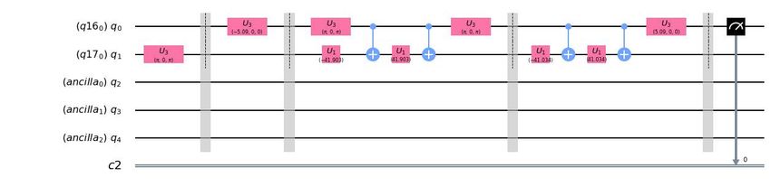
Simulation of non-radiative energy transfer in photosynthetic systems using a quantum computer

resonance energy transfer" (FRET), which applies to an irreversible hopping of an exciton from the donor to the
acceptor. The FRET rate (transition probability per unit time) can be expressed by the following relation [35]:
                                                           +∞
                                               J2
                                                       Z
                                         kF =                   dωLD (ω)IA (ω)                                      (2)
                                              2π~2       −∞

where J is the coupling constant, ω is the angular frequency of the electromagnetic field and LD (ω) and IA (ω)
denote dimensionless lineshape functions of the donor and acceptor molecules, directly related to the energy spec-
trum of each molecule. The integral is called the spectral overlap between the molecules. The coupling constant,
in the dipole-dipole approximation, is given by [3]:

                                         1
                              J=             [((d A · n) · d D ) − 3(dA · n)(dD · n)]  ,                       (3)
                                      η 2 R3
where η is the refractive index of the medium, dD (dA ) is the transient dipole moment of the donor (acceptor)
molecule, n = R/R, R is the radius vector between the two molecules and the angular brackets stand for angular
average over different orientations of the dipoles.
    Even though Eq. (2) (and the approach itself) is too simplistic to describe all possible situations in EET, defining
this characteristic transfer rate allows for the formulation of the following conditions for FRET to occur:

    • If the difference between the energy of the excited state energy of the donor (0 ) and acceptor (1 ) molecules
      is small, |0 − 1 |  J and they are in resonance, the energy transfer between the molecules can occur with
      a high probability;

    • If |0 − 1 |  J (off-resonance), the exciton is trapped in the donor molecule because it has a very low
      probability of being transferred; in this case it either stays in the molecule and later the donor molecule will
      decay to the ground state, dissipating the energy, or transfer the energy to a different acceptor nearby.

     As pointed out above, the initial idea of Förster was that an exciton is irreversibly transferred from a donor
to an acceptor. More recently, it has been shown experimentally that quantum coherent transport, where energy
is transported in the form of wave-packets, has a significant role in many important physical effects, including the
photosynthesis [9, 10, 39]. The Förster theory does not apply in this regime, as it simply ignores coherence. Later, in
1957, A. Redfield [43] proposed a transport theory, which applies to the opposite regime of strong coupling between
the donor and acceptor [9, 31, 35] (although originally it appeared in the context of NMR spectroscopy). Within
this concept, the exciton forms a coherent state based on the whole donor-acceptor pair and oscillates between the
two molecules. This system can be described by the following Hamiltonian:
                                           1
                                           X
                                   ĤS =         m |mi hm| + J (|0i h1| + |1i h0|) ,                               (4)
                                           m=0

where |mi denotes the exciton on the molecule m. The eigenstates of (4) are linear combinations of |0i and |1i.
Coherent dynamics corresponds to the presence of non-zero off-diagonal elements in the density matrix describing
the evolution of the quantum system. Their oscillation (or quantum beating) is indicative of coherence [35]. For
the system with Hamiltonian (4), the description in terms of state vectors is perfectly possible but it will not be
the case if interactions with environment are taken into account. Therefore, we may introduce the density matrix
description at this point. The evolution of the off-diagonal elements of the system’s density matrix, written in the
energy basis (where the Hamiltonian is diagonal) and denoted ρij , is given by:
                                               √         2   2
                                 ρij (t) = e−it (0 −1 ) +4J /~ ρij (0) ,   i 6= j .                            (5)

(see Supplementary Information A.2 for the derivation). These states are perturbed by interactions with the environ-
ment (the bath), which destroys their coherence. Mathematically, it is expressed in the form of a master equation,
which is known as the Bloch-Redfield equation; its general form can be found e.g. in Ref. [26].

                                                            4
Simulation of non-radiative energy transfer in photosynthetic systems using a quantum computer

    This consideration is extendable to a chain of molecules and can be seen as (partially) coherent transport [9].
The presence of the latter, observable through coherent oscillations of the energy levels of molecules across dif-
ferent sites (the quantum beating), was first conjectured in the 30’s [40] and theoretically predicted in more recent
works [28, 31]. It became possible to observe them more recently, thanks to the advances of optical spectroscopy
techniques [14, 23, 30, 53], and it was achieved even at room temperature [39]. In these experiments, it was pos-
sible to confirm the substantial impact of such coherent effects on the excitation energy transfer in photosynthetic
systems [35]. Moreover, the importance of environmental noise in the quantum transport involving coherence was
also discussed more recently [6, 42] and it is not fully understood yet.

Decoherence
Processes caused by the molecules’ environment may destroy coherence and thus influence this type of energy
transport [35, 36, 42], moreover, they can foster it. Indeed, completely coherent oscillations (called Rabi floppings
in atomic physics) between different molecular sites do not correspond to an energy flux. Breaking the oscillatory
evolution at some moment may help transferring the exciton along the molecular chain.
    If interactions exist between a system and its environment, they affect the (pure) states of the system, introducing
"errors" and making these states mixed. It means the so-called phenomenon of decoherence, which, by the way, has
been the main obstacle to the success of quantum computation. Decoherence processes can be divided into three
categories: (i) amplitude damping, (ii) dephasing, and (iii) depolarization, which are briefly described below.[5]
    Amplitude damping. Environment interactions with the system may cause a loss of the amplitude of one or
more system’s states. The spontaneous emission of a photon from the system (i.e. from one of the molecules) to the
environment is an example of this kind of process, so that the system returns to its ground state (without exciton)
[38]. For a two level system (e.g. a qubit), this type of decoherence contracts the Bloch sphere along the z axis (see
Supplementary Information A.1).
    Phase damping or dephasing. Such interactions conserve the energy of the system, contrary to the amplitude
damping. A phase damping channel removes the superposition of the system state, i.e. the off-diagonal terms
of the system’s density matrix decay over time down to zero. It is a process of removing the coherence of the
system, causing a classical probability distribution of states and, therefore, imposing some classical behaviour in a
quantum system. A simple way to look at this type of decoherence is also to think of the system interacting with
the environment where the relative phases of the system’s states become randomized by the environment. This
randomness comes from a distribution of energy eigenvalues of the environment. As a result, the evolution of the
quantum system’s Rabi cycle ceases but the time-average populations of the states may not change and this is the
case of the pure dephasing. For a two-level system with a pure dephasing interaction, the Bloch sphere contracts in
the x − y plane.
    Depolarization. This type of decoherence changes system’s state, which initially is pure, to a mixed state, with
a probability P of another pure state and the probability (1 − P ) of the initial state of the system. It is equivalent to
saying that, for a single qubit, an initial pure state represented on the Bloch sphere has suffered a contraction over
all dimensions of the sphere (with the contraction degree that depends on the probability P ). It can be thought of
as a combination of the other two types of decoherence.
    The amplitude damping is certainly detrimental for EET since the energy is simply dissipated into the envi-
ronment. The action of dephasing processes progressively eliminates the coherence (off-diagonal) elements in the
system’s density matrix, causing the oscillation amplitude to decay (beating supression). It eventually turns the
diagonal matrix elements (populations) into (non-correlated) classical probabilities, a process known as thermal
relaxation, for which the existence of coherence in a system is time limited. On the other hand, it has also been
shown that dephasing processes can have a positive role in the coherent transport of energy [35]. First, it yields ran-
dom fluctuations in the energy spectrum of each molecule, which can bridge the energy gap between the molecules,
momentarily turning a non resonant system into a resonant one. Secondly, dephasing can also help avoiding the
existence of the so called coherence traps in a molecular chain, a kind of deadlocks in energy transport where the

                                                            5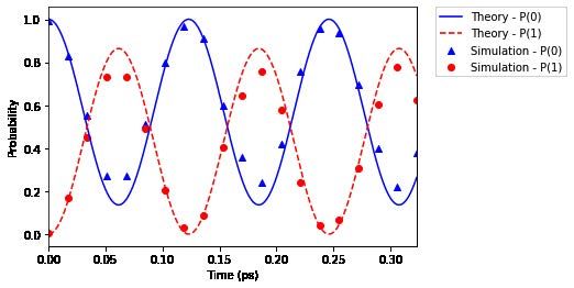
Simulation of non-radiative energy transfer in photosynthetic systems using a quantum computer

exciton can be confined [35]. Thus, the result of action of a decoherence source on an EET system is not obvious
a priori. Below we shall consider a simple model of pure dephasing consisting in a telegraph-type classical noise
affecting the donor-acceptor pair.

Materials and Methods
We aim at exploring the energy transport underlying the photosynthesis, throughout time, under two regimes: (i) in
an isolated system and (ii) under an action of the environment causing decoherence. In the "no decoherence" case
(i), one can study the evolution of system’s state vector, which obeys the equation

                                       |Ψtf i = e−iĤ(tf −ti )/~ |Ψti i ≡ Û |Ψti i                                  (6)

for a time-independent Hamiltonian. Here tf and ti are the upper and lower limits of the time interval to study. In
order to be able to do the calculation of the system’s evolution on a quantum computer, it is necessary to provide
a suitable qubit encoding for the possible states and an approximation for the Hamiltonian evolution operator, Û ,
in terms of quantum gates and circuits (computational Hamiltonian). The time, a continuous entity in equation (6),
has to be discretized onto a set of intervals, ∆t, where the Hamiltonian of interest can be approximated as constant.
The actual computational process is given by the repeated application of the evolution operator on the prepared
state |Ψi i, for s times, of the computational Hamiltonian, such that ti + s · ∆t = tf . The process is finished by the
observation of the desired properties, i.e. a set of measurements, in the appropriate basis, on the end state.
    Concerning the particular qubit encoding chosen, a chain of N = 2q molecules is encoded by a set of q qubits,
where |mi corresponds to the excitation (exciton) on the m-th molecule, e.g. for a two-molecule chain, state
|0i represents the exciton on the first molecule and |1i on the second one, and a possible successful transport of
energy would correspond to the transition of the state |0i to the state |1i. We denote this as the site basis. The
computational Hamiltonians under this encoding for the cases under study are discussed in the following sections.
From now on, we shall set ~ = 1. Also, it is convenient to measure the energies/frequencies in cm−1 , as it is
common in spectroscopy.

No–decoherence Hamiltonian
Considering a small chain of N molecules, the system’s Hamiltonian in the site basis reads as follows,

                                             N
                                             X −1                  X
                                     ĤS =          m |mi hm| +          Jmn |mi hn|                                (7)
                                             m=0                   m6=n

where m is the first excited state energy of the molecule m and Jnm is the electronic coupling between the
molecules n and m. The Hamiltonian (7) for just two molecules (1 qubit), identical to Eq.(4), in the 2 × 2 matrix
form, reads:
                                                                      !
                                                            0   J
                                                    ĤS =                 .                                          (8)
                                                            J    1

Its evolution operator is given by

                                      |Ψ(t)i = e−iĤS t |Ψ(0)i ≡ Û (t) |Ψ(0)i .                                     (9)

Although the Hamiltonian (44) possesses non-diagonal elements, finding a good approximation in terms of quantum
circuits is relatively straightforward. A possible strategy for this is by finding a diagonalizing transformation, T , of
the Hamiltonian, such that,

                                                            6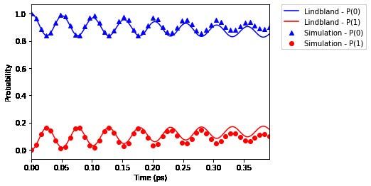
Simulation of non-radiative energy transfer in photosynthetic systems using a quantum computer

                                                           ĤS = T † ĤS−diag T .                                                    (10)
where ĤS−diag is the diagonal Hamiltonian. Therefore, the evolution operator can be rewritten as follows:

                                              Û (t) = e−iĤS t = T † e−iĤS−diag t T .                                              (11)
The problem now reduces to the approximation of the T operator (and its adjoint) and the Hamiltonian ĤS−diag ,
which can all be efficiently approximated in quantum circuits. The latter operator is diagonal in the site basis, thus
the unitary evolution operator can be expressed as
                                                                                                    "   1
                                                                                                                           #
                                                           h            P1           i                  Y
                                        −iĤS t        †           −i    m=0 Em t               †                 −iEm t
                           Û (t) = e             =T           e                         T =T                 e                T .   (12)
                                                                                                        m=0

The T and T † matrices can be implemented by simple rotations, Ry (θ) and Ry (−θ), for a two-molecule system.
However, for a higher number of molecules, a rotational decomposition algorithm together with the Gray code
[38], which decomposes a matrix in the multiplication of a single qubit and CNOT gates, has to be used. Using
this particular algorithm the gate complexity for N molecules is O(N 2 log 2 [N ]) [38]. On the other hand, the
diagonalized evolution operator,
                                                                    !
                                                   e−iE0 t    0
                                         Û (t) =                     ,                                    (13)
                                                     0      e−iE1 t
translates into trivial phase rotations over each of the energy eigenstates |Ei i of the system with the respective
energy eigenvalues Ei . This operator can be constructed as a sequence of CRZ (φi ) gates applied to an ancilla
qubit (initialized at |1i), where the angle is given by φi = −2Ei t, i = 1, 2. The X gates are used to "select" the
eigenvector to which the controlled rotation is to be applied. The circuit implementation of the operator defined in
(13) is illustrated in Figure 2. The gate complexity of this operator, in terms of single qubit and CNOT gates for N
molecules, is O(N log[N ]).

              |qsystem i         X                     •                         X                            •

                 |1ianc                       RZ (−2E00 t)                                          RZ (−2E10 t)

Figure 2: Implementation of the system’s evolution operator. |qsystem i is the state vector of the system’s qubit in
the energy eigenbasis.

For the whole circuit, resulting from the sequencing of T † ĤS−diag T , the number of qubits required to simulate a
molecular chain of N elements is 2 log2 N and the gate count scales with O(N 2 log22 N ) single qubit and CNOT
gates. The transformations T and T † , in the general case, possess a high circuit depth, which makes the system
hard to simulate accurately, with low error rate, in the current available quantum computers.

Introducing decoherence into the system
We shall implement artificial decoherence as pure-dephasing by adding Markovian fluctuations to the Hamiltonian.
This approach is considered a good approximation in the high-temperature regime for the bath [5, 31, 42]. The
actual algorithm to be used is the one of [55], which is used to simulate open quantum systems, with pure dephasing,
modeling the action of the decoherence as classical random fluctuations (a telegraph-type classical noise affecting
the system). The actual Hamiltonian for this system reads as

                                                                   Ĥ = ĤS + ĤF                                                    (14)

                                                                             7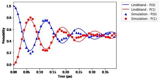
Simulation of non-radiative energy transfer in photosynthetic systems using a quantum computer

and it consists of the system Hamiltonian, ĤS , of the previous section and the perturbation of a bi-stable fluctuator
environment, ĤF . The latter simply shifts the energy by a constant value for each molecule, ±gm /2, as illustrated
in Fig. 3. Explicitly,
                                                        X1
                                                ĤF =       χm (t)Âm                                              (15)
                                                       m=0

where Âm |mi hm| is the projection operator and considering one fluctuator interacting with each molecule m,

                                                 χm (t) = gm ξm (t) .                                                               (16)

The function ξm (t) switches the fluctuator between the positive and negative values (appearing randomly) at a given
fixed rate γ and gm is the fluctuation strength (or the coupling strength to a molecule m). Physically, the action
of the fluctuations is typically stronger for the excited states [1, 31] and g can be larger than the donor-acceptor
coupling J.

Figure 3: Uncorrelated random fluctuations applied to donor and aceptor’s excited state energies, 0 and 1 . Each
molecule is affected by one fluctuator, which generates a telegraph-type classical noise. The fluctuators switch
randomly between the positive and negative value at a given fixed rate, so that the periods of time when the molecule
energy is constant, m + gm /2 or m − gm /2, are random. J is the coupling strength between the molecules that
can be seen as the rate of hoppings between these fluctuating energy levels.

The implementation of such random bi-valued function ξm (t), can be done in a straightforward way by a classical
pseudo-random numbers generator with a probability of 50% of the values −1/2 and 1/2. For circuit generation
purposes, the values resulting from the random sampling have to be provided in advance of the quantum simulation.
     The fluctuator interaction Hamiltonian and the system Hamiltonian do not commute, so, in order to generate an
appropriate quantum circuit, one needs to apply an approximation technique such as the Trotter product formula
[56]. Under this approximation, the unitary evolution operator of the Hamiltonian, for a time t = Ni ∆t, where Ni
is the number of iterations and ∆t is the iteration time-step, becomes

                                                                        "   1
                                                                                                    #        "   1
                                                                                                                            # !Ni
                         Ni                                Ni
                                                                                      ±i g2m
                                                                            Y                                    Y
   U (Ni ∆t) = e−iĤ∆t          = e−iĤF ∆t T † e−iĤS ∆t T         =             e            ∆t
                                                                                                        T†           e−iEm ∆t T     ,
                                                                            m=0                              m=0
                                                                                                                  (17)
where Em denote the eigenvalues of the system Hamiltonian.
     Note that the projection operator Âm is not present in the evolution operator (17) because the latter is used in
                                                                                       gm
its eigenbasis, i.e. the site basis. The fluctuator interaction evolution operator e±i 2 ∆t is a selective rotational
gate over a molecule m (|mi), which can be implemented by a set of X gates and a controlled gate CRZ (φm ) with
angle φm = ±gm ∆t, applied over an ancilla qubit initialized at |1i. The whole circuit is presented in Fig. 4 for
one iteration. The fluctuator waiting time (interval of time between switches), i.e. γ1 , can only be equal or higher
than the iteration time-step, ∆t. The switching in the fluctuator-molecule coupling strength is performed at every
  1                             1
γ∆t iterations, where a∆t = γ , a ∈ N.

                                                              8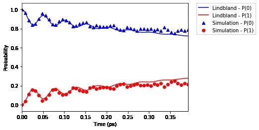
Simulation of non-radiative energy transfer in photosynthetic systems using a quantum computer

                 Usually in the study of open quantum systems with a dilated system’s Hilbert space (as is the case here),
             different measurement techniques are required [38, 55], however in this case, the open system is simulated in
             a closed form so, similarly to the no decoherence case, the measurement over the site basis suffices. The full
             algorithm (random values generator plus the actual simulation) must be performed several times, so that the results
             of all runs are averaged.
                 Let us consider the simulation for a time t, using an iteration time step ∆t, and assuming that the environment
             can have more than one fluctuator interacting with each molecule as well as the chain can have more than just two
             elements. Then the fluctuator interaction evolution operator requires the following gate resource complexity for a
                              t
             single run: O( ∆t  [N (log2 N + F )]) single qubit and CNOT gates, where N is the number of molecules and F is
             the number of fluctuators interacting with each one.

|qsystem i      Ry (θ)   X           •         X            •                Ry (−θ)   X        •         X          •

   |1ianc                     RZ (−2E00 ∆t)           RZ (−2E10 ∆t)                        RZ (±g 0 ∆t)        RZ (±g 0 ∆t)

             Figure 4: Implementation of one iteration of the system with decoherence algorithm. Here |qsystem i represents the
             system’s qubit state vector in the site basis.

                                                                                                                          t
                 In the implementation of the system with decoherence, the algorithm gate resources complexity is O( ∆t     [N 2
             × log22 N + N F ]) for a single run. This simulation, yet again, possess a very high circuit depth which makes its
             application unfeasible in quantum computers. The number of necessary qubits is the same as in the no decoherence
             simulation (2 log2 N ).
                                         PF
                 It also requires O(N R j=0 tγj ) random numbers to be classically generated, where R is the number of runs
             of the algorithm and γj is the switching rate of the fluctuator j interacting with the molecule. The number of
                                                                                                                      t 2 2

             required simulation runs to average the results and obtain an error  > 0, is predicted to scale as O [F ∆t ] / .
             This complexity is calculated based on the possible non-degenerate energy state outcomes of the entire chain in the
             simulation for a time t. These outcomes are caused by the bi-stable random fluctuations, therefore, the possible
             non-degenerate energy state outcomes for each molecule obey a discrete Gaussian probability distribution.

             Results
             We conducted simulation experiments for the quantum transport in a molecular chain using the algorithm described
             in the previous section. We executed the simulation for the coherent system on a real quantum computer, the IBM
             Q of 5 qubits, while the pure dephasing scenario was simulated on the QASM quantum simulator, both in the near-
             resonant and non-resonant regimes. For the validation purposes, we compared the results for the coherent system
             with the theoretical predictions obtained by solving the Schrödinger equation (see Supplementary Information A.2).
                 As for the decoherent regime, we used a classical computation of the stochastic Haken-Ströbl model [22, 42].
             The simulations and circuits involved, encoded in the Qiskit platform [11], can be performed in the following url:
             https://github.com/jakumin/Photosynthesis-quantum-simulation.

             Coherent regime
             The scenario for this regime was simulated with a simple chain of two molecules. As discussed in section Materials
             and Methods and using the parameters as proposed in [54], we define the system’s Hamiltonian as follows:
                (Near-resonant regime)                                       !
                                                                13000        126
                                                     HS =                         cm−1 ;                                   (18)
                                                                 126        12900

                                                                        9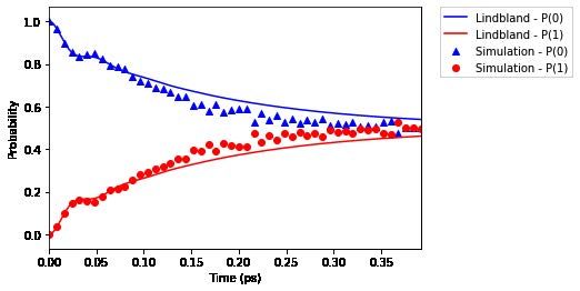
Simulation of non-radiative energy transfer in photosynthetic systems using a quantum computer

   (Non-resonant regime)                                       !
                                                 12900     132
                                        HS =                     cm−1 .                                       (19)
                                                  132     12300
The results for both regimes were obtained using an actual quantum device (the IBMQ london of 5 qubits) and can
be seen in Figs. 5 and 6, respectively. Due to the stochastic nature of quantum computers, the experiments were
conducted with 2048 shots for each time value. The specific optimized quantum circuits used in this experiment
are presented in Supplementary information A.3. In the following results, the probability of the donor and acceptor
molecules being excited is denoted by P (0) = h0| ρS (t) |0i and P (1) = h1| ρS (t) |1i, respectively.

Figure 5: Evolution dynamics of the isolated system obtained by employing the quantum algorithm for the near-
resonant system: simulation results (points) and theory (lines).

Figure 6: Evolution dynamics of the isolated system obtained by employing the quantum algorithm for the non-
resonant system: simulation results (points) and theory (lines).

    Taking the fluctuator’s switching rate to be γ = 0 or the fluctuator-molecule coupling strength to be g = 0,
one has the coherent regime. These simulations show the limiting case of the Redfield regime, i.e. the very weak
system-environment coupling, g  J. The quantum beatings, observed in the simulation results, can be thought
of as a reversible transfer of energy between the molecules, where the excitation goes back and forth across the
molecules [8].
    In the performed simulations, the near-resonant and non-resonant regimes have a maximum probability of
∼ 90% and ∼ 20%, respectively, of the energy being transferred to the acceptor molecule. Using the quantum

                                                         10
Simulation of non-radiative energy transfer in photosynthetic systems using a quantum computer
Liouville equation [35] (see Supplementary information A.2), the period of the quantum beating is Tnear−res ≈
123 f s for the near-resonant regime and Tnon−res ≈ 51 f s for the non-resonant regime. These periods are in
the femtosecond timescale of the experimentally observable quantum beatings [10, 14, 39]. The simulation results
show a similar behaviour as those predicted by the Schrödinger and quantum Liouville equations, where the off
curve points are predominantly originated by errors in the quantum hardware.
Decoherent regime
The scenario for the regime with decoherence introduced is, in some respect, similar to the one presented for the
coherent regime for a chain of two molecules. No further changes are made to the Hamiltonian discussed in the
section Introduction of decoherence in the system. The quantum simulation results are compared with a theoretical
evolution based on the stochastic Haken-Ströbl model, in the form of the Lindbland master equation [22, 42].
The Lindbland equations were solved in a classical computer using Qutip [27], a quantum open systems software
framework. The set of Lindbland equations, correspondent to the model in this setting, had one free parameter
regarding the environment, the dephasing rate, γdeph . The Lindbland equation in the Haken-Ströbl model reads:
dρ X 1 1
= L[ρ] = −i[HS , ρ] + γdeph (Lm ρ(t)L†m − ρ(t)L†m Lm − L†m Lm ρ(t)) (20)
dt m
2 2
where Lm = |mi hm| are the Lindbland operators, responsible for the system-environment interaction. The system
Hamiltonian, HS , is given by the matrix (18) for the near-resonant system and the matrix (19) for the non-resonant
system.
For each quantum simulation performed, a fitting process has been employed by adjusting the dephasing rate
of the Haken-Ströbl model, so that the system’s evolution in both classical and quantum algorithms have similar
behaviours. This enables one to perform a direct comparison between both theories and to find the actual dephasing
rate of the modeled environment over the various regimes considered in this work.
The environment contains only one fluctuator interacting with each molecule with switching rate γ = 125
THz. As mentioned above, the dephasing rate, γdeph , for the Lindbland equation is adjusted to the behaviour of the
system under the action of a fluctuation strength g. For a range of fluctuation strengths of [100, 1000] cm−1 , in the
quantum algorithm, and the corresponding dephasing rate of the Haken-Ströbl model lies in the ∼ [2.3, 70] THz
range. Due to the existence of random fluctuations, large number of samples had to be generated. The algorithm
was implemented with 250 runs, where 5000 shots were performed for each time t. Figures 7 and 8 present the
simulation results for different values of the fluctuation strength, along with the theoretical evolution dynamics, for
the near-resonant and non-resonant systems, respectively.
11Simulation of non-radiative energy transfer in photosynthetic systems using a quantum computer
(a) g = 100 cm−1 , γdeph = 2.3 T Hz. (b) g = 300 cm−1 , γdeph = 10 T Hz.
(c) g = 700 cm−1 , γdeph = 41 T Hz. (d) g = 1000 cm−1 , γdeph = 70 T Hz.
Figure 7: Evolution dynamics of the system with decoherence obtained by employing the quantum algorithm for
the near-resonant system: simulation results (points) and theory (lines).
12Simulation of non-radiative energy transfer in photosynthetic systems using a quantum computer
(a) g = 100 cm−1 , γdeph = 2.3 T Hz. (b) g = 300 cm−1 , γdeph = 10 T Hz.
(c) g = 700 cm−1 , γdeph = 41 T Hz. (d) g = 1000 cm−1 , γdeph = 70 T Hz.
Figure 8: Evolution dynamics of the system with decoherence obtained by employing the quantum algorithm for
the non-resonant system: simulation results (points) and theory (lines).
It is seen in Figures 7 and 8 that oscillation amplitudes decay over time, as expected, due to the loss of relative
phase coherence between the excited states of the two molecules, evidenced by the disappearance of the quantum
beatings. This is associated with the irreversible evolution when the system loses its capacity of performing coher-
ent transport. Additionally, it is clear that the system is led to a classical distribution of the populations in the site
eigenbasis.
In the regime under the study, where the environment is assumed to be at thermal equilibrium, the final
probability distribution is calculated in the limit of the classical Boltzmann distribution hm| ρS (t → ∞) |mi =
− m
const × e kB T . Here kB is the Boltzmann constant, T is the temperature of the bath and const is a normalization
constant [5]. Taking the limit of very high temperatures, the population terms approach the Boltzmann distribution
h0| ρS (t → ∞) |0i ≈ h1| ρS (t → ∞) |1i ≈ 21 , which is compatible with the results obtained. The relaxation can
not be fully observed in Figs. 7a, 8a and 8b because a very large number of iterations would be required for this.
The switching rate must be high enough to observe the dephasing effects. Here we used a value ≈ 33 times
larger than the transfer rate, J (that is, the fluctuator waiting time must be shorter than J −1 ). As observed in the
simulations, it is a suitable value for observing the relevant effects of random fluctuations in the system. At very
low rates, it leads the system’s evolution to a behaviour similar to the previously observed in the no-decoherence
regime, Figs. 5 and 6.
The time that coherence lasts in the system is essentially defined by the fluctuation strength, g: in Figs. 7a,
7b, 8a and 8b (lower g) the coherence is maintained for some time, while in Figures 7c, 7d, 8c and 8d (higher
g) it is quickly suppressed. In the latter regime, an approximated diffusive motion drives the system’s evolution,
where quantum beating is practically absent. The time that the quantum beating lasts in these simulations (until it
reaches an approximate non-oscillating behaviour), is about 350 f s in Figure 7b (near-resonant system) and 200
f s in Figure 8b (non-resonant system), with a fluctuation strength g = 300 cm−1 . At a longer time, it has been
13Simulation of non-radiative energy transfer in photosynthetic systems using a quantum computer
experimentally observed to persist (t > 660 f s [39]), a timescale which could be modeled in the present simulation
by changing the environment parameters, i.e. lowering the fluctuation strength g as can be observed in Figures 7a
and 8a.
Discussion and Conclusions
Two main conclusions can be drawn from the presented results:
• There is a very good agreement between the solution of the Schrödinger equation and the coherent quantum
algorithm results in the reproduction of the purely oscillatory evolution of the isolated quantum system.
• There also is a good agreement between the results obtained by the Haken-Ströbl model and the quantum
algorithm. The increase of the dephasing rate imply an increase in the fluctuation strengths thus, a faster
suppression of the quantum beatings can be observed, as predicted theoretically [42].
Therefore, the correctness of the results obtained in the quantum simulations is verified.
The results obtained in the present work were not directly compared with Ref. [54], due to the different
timescales used. The major difference lies in the physical implementation, NMR vs universal quantum computer,
where there might be an advantage for the former from the point view of the scalability and reliability, at the cur-
rent state of quantum technology. However, there is a clear advantage of the quantum computer, from the point
of easiness of implementation, as it is also possible to implement circuits of arbitrary precision, harder to do with
the NMR simulator, which is dependent on a Hamiltonian mapping process. The computational advantage ver-
ified for the NMR simulator still holds after the present work, as the number of executions for the algorithm of
this work is polynomial on the precision required, although the circuit generation maybe problematic, as a matrix
diagonalization operation is necessary (complexity estimated in O(N 3 )).
To conclude, we proposed a quantum algorithm to simulate the energy transfer phenomenon present in gen-
eral photosynthesis, under the presence of quantum coherence between the molecules and the decoherence effects
caused by environmental interference. Using this algorithm we also performed simulations in the commercially
available quantum computer of IBM, the IBM Q of 5 qubits for the coherent scenario and in the quantum simulator
(QASM) for the decoherent scenario. For validation purposes, we also computed the evolution of analogous sys-
tems using well-established (classical) methods in literature, obtaining quite similar results between the methods.
The results obtained were also in agreement with the predictions that can be found in literature, for the role of
the quantum coherent and dephasing effects in the energy transport of photosynthesis: for the high temperature
environment here defined, it was clear that dephasing, modelled as energy fluctuations in the site energies, limited
the time quantum coherence lasts in light-harvesting antenna. Moreover, it was also verified that the fluctuation
strength and the switching rate of the Markovian fluctuator environment are directly related with the energy transfer
efficiency, allowing the simulation of different transport regimes by setting them appropriately.
Similar to Ref. [54], this setting revealed itself as an interesting platform for the study the quantum and envi-
ronmental effects in a small photosynthetic system, and therefore we consider, that the use of quantum simulations
may be a feasible alternative in systems with medium-strong coupling and non-Markovian systems, in the future.
However, the algorithm obtained, due to the high requirements of gates and qubits, is not scalable to real world
photosynthetic systems, with the current state of quantum technology. Hence, this simulation should be seen as a
proof of concept, since a realistic quantum simulation of a photosynthetic system would have to involve hundreds
of light-harvesting molecules, which is beyond the current quantum technology. Furthermore, the algorithm only
effectively simulates pure-dephasing baths. For future work, we aim at extending it to new types of bath, e.g.
those allowing for higher exciton recombination rates and non-Markovian effects as well as to new geometries of
photosynthetic systems, in particular, to the Fenna-Matthews-Olson complex [35].
14Simulation of non-radiative energy transfer in photosynthetic systems using a quantum computer
Competing Interests
The authors declare that there are no conflicts of interest.
Acknowledgements
Carlos Tavares was funded by the FCT – Fundação para a Ciência e Tecnologia (FCT) by the grant SFRH/BD/116367/2016,
funded under the POCH programme and MCTES national funds. This work is also financed by the ERDF – Euro-
pean Regional Development Fund through the Operational Programme for Competitiveness and Internationalisation
- COMPETE 2020 Programme and by national funds through the Portuguese funding agency, FCT - Fundação
para a Ciência e a Tecnologia, within project KLEE (POCI-01-0145-FEDER-030947) and the Strategic Funding
UIDB/04650/2020 of the Centre of Physics.
References
[1] Julia Adolphs and Thomas Renger. How proteins trigger excitation energy transfer in the fmo complex of
green sulfur bacteria. Biophysical Journal, 91(8):2778–2797, 2006.
[2] Qing Ai, Tzu-Chi Yen, Bih-Yaw Jin, and Yuan-Chung Cheng. Clustered geometries exploiting quantum
coherence effects for efficient energy transfer in light harvesting. The Journal of Physical Chemistry Letters,
4(15):2577–2584, 2013.
[3] D. L. Andrews and B. S. Sherborne. Resonant excitation transfer: A quantum electrodynamical study. Journal
of Chemical Physics, 86:4011 – 4017, 1987.
[4] Stephen Barnett. Quantum information, volume 16. Oxford University Press, 2009.
[5] Heinz-Peter Breuer, Francesco Petruccione, et al. The theory of open quantum systems. Oxford University
Press on Demand, 2002.
[6] Jianshu Cao and Robert J Silbey. Optimization of exciton trapping in energy transfer processes. The Journal
of Physical Chemistry A, 113(50):13825–13838, 2009.
[7] YC Cheng and Robert J Silbey. Coherence in the b800 ring of purple bacteria lh2. Physical Review Letters,
96(2):028103, 2006.
[8] Yuan-Chung Cheng, Gregory S Engel, and Graham R Fleming. Elucidation of population and coherence
dynamics using cross-peaks in two-dimensional electronic spectroscopy. Chemical Physics, 341(1-3):285–
295, 2007.
[9] Aurélia Chenu and Gregory D Scholes. Coherence in energy transfer and photosynthesis. Annual Review of
Physical Chemistry, 66:69–96, 2015.
[10] Elisabetta Collini, Cathy Y Wong, Krystyna E Wilk, Paul MG Curmi, Paul Brumer, and Gregory D Sc-
holes. Coherently wired light-harvesting in photosynthetic marine algae at ambient temperature. Nature,
463(7281):644–647, 2010.
[11] Andrew Cross. The ibm q experience and qiskit open-source quantum computing software. Bulletin of the
American Physical Society, 63, 2018.
[12] Johann Deisenhofer and Hartmut Michel. The photosynthetic reaction center from the purple bacterium
rhodopseudomonas viridis. Science, 245(4925):1463–1473, 1989.
15Simulation of non-radiative energy transfer in photosynthetic systems using a quantum computer
[13] Roberto Di Candia, Julen S Pedernales, Adolfo Del Campo, Enrique Solano, and Jorge Casanova. Quantum
simulation of dissipative processes without reservoir engineering. Scientific Reports, 5(1):1–7, 2015.
[14] Gregory S Engel, Tessa R Calhoun, Elizabeth L Read, Tae-Kyu Ahn, Tomáš Mančal, Yuan-Chung Cheng,
Robert E Blankenship, and Graham R Fleming. Evidence for wavelike energy transfer through quantum
coherence in photosynthetic systems. Nature, 446(7137):782–786, 2007.
[15] Richard P Feynman. Simulating physics with computers. Int. J. Theor. Phys, 21(6/7), 1982.
[16] Richard Phillips Feynman and FL Vernon Jr. The theory of a general quantum system interacting with a linear
dissipative system. Annals of Physics, 24:118–173, 1963.
[17] Graham R Fleming and Rienk Van Grondelle. The primary steps of photosynthesis. Physics Today, 47(2):48–
57, 1994.
[18] Theodor Förster. Delocalized excitation and excitation transfer. Florida State University, 1965.
[19] Iulia M Georgescu, Sahel Ashhab, and Franco Nori. Quantum simulation. Reviews of Modern Physics,
86(1):153, 2014.
[20] Devens Gust, Thomas A Moore, and Ana L Moore. Mimicking photosynthetic solar energy transduction.
Accounts of Chemical Research, 34(1):40–48, 2001.
[21] Devens Gust, Thomas A Moore, and Ana L Moore. Solar fuels via artificial photosynthesis. Accounts of
Chemical Research, 42(12):1890–1898, 2009.
[22] Hermann Haken and Gert Strobl. An exactly solvable model for coherent and incoherent exciton motion.
Zeitschrift für Physik A Hadrons and nuclei, 262(2):135–148, 1973.
[23] Richard Hildner, Daan Brinks, Jana B Nieder, Richard J Cogdell, and Niek F van Hulst. Quantum coherent
energy transfer over varying pathways in single light-harvesting complexes. Science, 340(6139):1448–1451,
2013.
[24] Akihito Ishizaki and Yoshitaka Tanimura. Nonperturbative non-markovian quantum master equation: Validity
and limitation to calculate nonlinear response functions. Chemical Physics, 347(1-3):185–193, 2008.
[25] Seogjoo Jang, Jianshu Cao, and Robert J Silbey. Fourth-order quantum master equation and its markovian
bath limit. The Journal of Chemical Physics, 116(7):2705–2717, 2002.
[26] Jan Jeske, David J Ing, Martin B Plenio, Susana F Huelga, and Jared H Cole. Bloch-redfield equations for
modeling light-harvesting complexes. The Journal of Chemical Physics, 142(6):064104, 2015.
[27] J Robert Johansson, Paul D Nation, and Franco Nori. Qutip: An open-source python framework for the
dynamics of open quantum systems. Computer Physics Communications, 183(8):1760–1772, 2012.
[28] Robert S Knox. Electronic excitation transfer in the photosynthetic unit: reflections on work of william arnold.
Photosynthesis Research, 48(1-2):35–39, 1996.
[29] Neill Lambert, Yueh-Nan Chen, Yuan-Chung Cheng, Che-Ming Li, Guang-Yin Chen, and Franco Nori. Quan-
tum biology. Nature Physics, 9(1):10–18, 2013.
[30] Hohjai Lee, Yuan-Chung Cheng, and Graham R Fleming. Coherence dynamics in photosynthesis: protein
protection of excitonic coherence. Science, 316(5830):1462–1465, 2007.
[31] Jan A Leegwater. Coherent versus incoherent energy transfer and trapping in photosynthetic antenna com-
plexes. The Journal of Physical Chemistry, 100(34):14403–14409, 1996.
16Simulation of non-radiative energy transfer in photosynthetic systems using a quantum computer
[32] Nathan S Lewis. Research opportunities to advance solar energy utilization. Science, 351(6271), 2016.
[33] Seth Lloyd. Universal quantum simulators. Science, pages 1073–1078, 1996.
[34] Christine Maier, Tiff Brydges, Petar Jurcevic, Nils Trautmann, Cornelius Hempel, Ben P Lanyon, Philipp
Hauke, Rainer Blatt, and Christian F Roos. Environment-assisted quantum transport in a 10-qubit network.
Physical Review Letters, 122(5):050501, 2019.
[35] Masoud Mohseni, Yasser Omar, Gregory S Engel, and Martin B Plenio. Quantum effects in biology. Cam-
bridge University Press, 2014.
[36] Masoud Mohseni, Patrick Rebentrost, Seth Lloyd, and Alan Aspuru-Guzik. Environment-assisted quantum
walks in photosynthetic energy transfer. The Journal of Chemical Physics, 129(17):11B603, 2008.
[37] Sarah Mostame, Patrick Rebentrost, Alexander Eisfeld, Andrew J Kerman, Dimitris I Tsomokos, and Alan
Aspuru-Guzik. Quantum simulator of an open quantum system using superconducting qubits: exciton trans-
port in photosynthetic complexes. New Journal of Physics, 14(10):105013, 2012.
[38] Michael A Nielsen and Isaac Chuang. Quantum computation and quantum information. Cambridge Univer-
sity Press, 2010.
[39] Gitt Panitchayangkoon, Dugan Hayes, Kelly A Fransted, Justin R Caram, Elad Harel, Jianzhong Wen,
Robert E Blankenship, and Gregory S Engel. Long-lived quantum coherence in photosynthetic complexes at
physiological temperature. Proceedings of the National Academy of Sciences, 107(29):12766–12770, 2010.
[40] Francis Perrin. Théorie quantique des transferts d’activation entre molécules de même espèce. cas des solu-
tions fluorescentes. In Annales de Physique, volume 10, pages 283–314. EDP Sciences, 1932.
[41] Anton Potočnik, Arno Bargerbos, Florian AYN Schröder, Saeed A Khan, Michele C Collodo, Simone Gas-
parinetti, Yves Salathé, Celestino Creatore, Christopher Eichler, Hakan E Türeci, et al. Studying light-
harvesting models with superconducting circuits. Nature Communications, 9(1):1–7, 2018.
[42] Patrick Rebentrost, Masoud Mohseni, Ivan Kassal, Seth Lloyd, and Alán Aspuru-Guzik. Environment-
assisted quantum transport. New Journal of Physics, 11(3):033003, 2009.
[43] Alfred G Redfield. On the theory of relaxation processes. IBM Journal of Research and Development,
1(1):19–31, 1957.
[44] David R Reichman and Robert J Silbey. On the relaxation of a two-level system: Beyond the weak-coupling
approximation. The Journal of Chemical Physics, 104(4):1506–1518, 1996.
[45] Elisabet Romero, Vladimir I Novoderezhkin, and Rienk van Grondelle. Quantum design of photosynthesis
for bio-inspired solar-energy conversion. Nature, 543(7645):355–365, 2017.
[46] J. R. Santos, M. I. Vasilevskiy, and S. A. Filonovich. Cascade upconversion of photoluminescence in quantum
dot ensembles. Physical Review B, 78:245422, 2008.
[47] DW Schönleber, Alexander Eisfeld, Michael Genkin, S Whitlock, and Sebastian Wüster. Quantum simulation
of energy transport with embedded rydberg aggregates. Physical Review Letters, 114(12):123005, 2015.
[48] Wolf-Dieter Schubert, Olaf Klukas, Norbert Krauß, Wolfram Saenger, Petra Fromme, and Horst Tobias Witt.
Photosystem i of synechococcus elongatus at 4 å resolution: comprehensive structure analysis. Journal of
Molecular Biology, 272(5):741–769, 1997.
[49] A Soare, H Ball, D Hayes, J Sastrawan, MC Jarratt, JJ McLoughlin, X Zhen, TJ Green, and MJ Biercuk.
Experimental noise filtering by quantum control. Nature Physics, 10(11):825–829, 2014.
17Simulation of non-radiative energy transfer in photosynthetic systems using a quantum computer
[50] Yoshitaka Tanimura. Stochastic liouville, langevin, fokker–planck, and master equation approaches to quan-
tum dissipative systems. Journal of the Physical Society of Japan, 75(8):082001, 2006.
[51] Yoshitaka Tanimura and Ryogo Kubo. Time evolution of a quantum system in contact with a nearly gaussian-
markoffian noise bath. Journal of the Physical Society of Japan, 58(1):101–114, 1989.
[52] Ming-Jie Tao, Ming Hua, Qing Ai, and Fu-Guo Deng. Quantum simulation of clustered photosynthetic light
harvesting in a superconducting quantum circuit. arXiv preprint arXiv:1810.05825, 2018.
[53] Rienk van Grondelle and Vladimir I Novoderezhkin. Energy transfer in photosynthesis: experimental insights
and quantitative models. Physical Chemistry Chemical Physics, 8(7):793–807, 2006.
[54] Bi-Xue Wang, Ming-Jie Tao, Qing Ai, Tao Xin, Neill Lambert, Dong Ruan, Yuan-Chung Cheng, Franco
Nori, Fu-Guo Deng, and Gui-Lu Long. Efficient quantum simulation of photosynthetic light harvesting. NPJ
Quantum Information, 4(1):1–6, 2018.
[55] Hefeng Wang, Sahel Ashhab, and Franco Nori. Quantum algorithm for simulating the dynamics of an open
quantum system. Physical Review A, 83(6):062317, 2011.
[56] Nathan Wiebe, Dominic Berry, Peter Høyer, and Barry C Sanders. Higher order decompositions of ordered
operator exponentials. Journal of Physics A: Mathematical and Theoretical, 43(6):065203, 2010.
[57] Lei Xu, ZR Gong, Ming-Jie Tao, Qing Ai, et al. Artificial light harvesting by dimerized möbius ring. Physical
Review E, 97(4):042124, 2018.
[58] Xing-Long Zhen, Fei-Hao Zhang, Guanru Feng, Hang Li, and Gui-Lu Long. Optimal experimental dynamical
decoupling of both longitudinal and transverse relaxations. Physical Review A, 93(2):022304, 2016.
18You can also read