Gravitational Lensing and Time Delay - Uni Bielefeld
←
→
Page content transcription
If your browser does not render page correctly, please read the page content below
BIELEFELD UNIVERSITY
                             FACULTY OF PHYSICS

                                   Master’s Thesis

                   Gravitational Lensing
                     and Time Delay

                                February 26, 2021

                                       Author
                              Shivani Deshmukh
                       sdeshmukh@physik.uni-bielefeld.de
                             Bielefeld University

Supervisor & First Referee                                        Second Referee
Prof. Dr. Dominik Schwarz                                  Dr. Yuko Urakawa
dschwarz@physik.uni-bielefeld.de                     yuko@physik.uni-bielefeld.de
Bielefeld University                                        Bielefeld University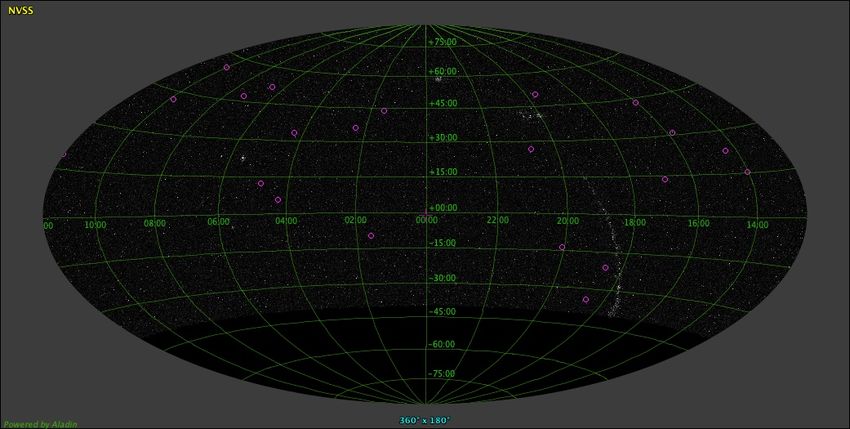
ii
Contents
1 Introduction 1
2 Basic Concepts 3
2.1 Cosmology and the Problem of Dark Matter . . . . . . . . . . . . . . 3
2.1.1 Robertson-Walker Metric . . . . . . . . . . . . . . . . . . . . . 3
2.1.2 Friedmann Equations . . . . . . . . . . . . . . . . . . . . . . . 4
2.1.3 Redshifts and Distances . . . . . . . . . . . . . . . . . . . . . 5
2.1.4 Missing Mass Problem . . . . . . . . . . . . . . . . . . . . . . 6
2.2 Gravitational Lensing . . . . . . . . . . . . . . . . . . . . . . . . . . . 8
2.2.1 Deflection Angle . . . . . . . . . . . . . . . . . . . . . . . . . 8
2.2.2 Lens Geometry and Lens Equation . . . . . . . . . . . . . . . 9
2.2.3 Magnification Factor . . . . . . . . . . . . . . . . . . . . . . . 11
2.2.4 Time Delay . . . . . . . . . . . . . . . . . . . . . . . . . . . . 12
3 Lens Models in Asymptotically Flat Spacetime 19
3.1 Schwarzschild Lens . . . . . . . . . . . . . . . . . . . . . . . . . . . . 19
3.2 Axially Symmetric Lens . . . . . . . . . . . . . . . . . . . . . . . . . 22
3.3 Perturbed Symmetric Lens . . . . . . . . . . . . . . . . . . . . . . . . 25
4 Mass Profile of Lenses 29
4.1 Singular Isothermal Sphere . . . . . . . . . . . . . . . . . . . . . . . . 29
4.2 Exponential Disk . . . . . . . . . . . . . . . . . . . . . . . . . . . . . 30
4.3 Navarro-Frenk-White density profile . . . . . . . . . . . . . . . . . . . 31
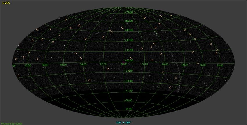
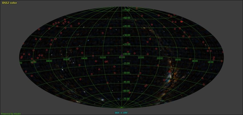
5 A Survey of Gravitationally Lensed Systems 33
5.1 Sky Surveys and Projects . . . . . . . . . . . . . . . . . . . . . . . . 33
5.2 Gravitationally Lensed Quasar Catalog . . . . . . . . . . . . . . . . . 37
6 Conclusion 45
Bibliography 47
iii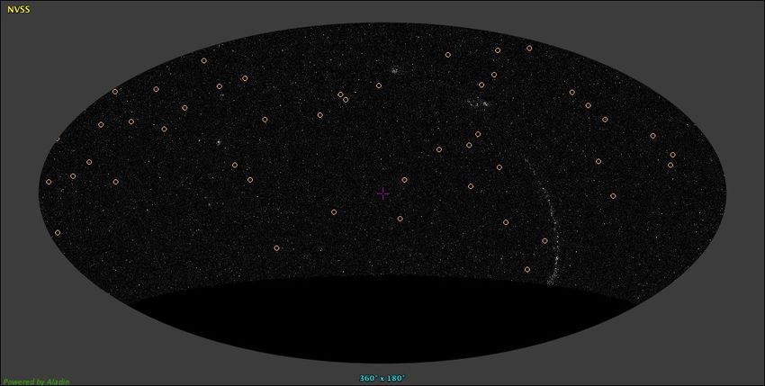
iv CONTENTS
Chapter 1

Introduction

Historical Aspect
A consequence of Albert Einstein’s theory of general relativity is gravitational lens-
ing. In recent years the true scope and importance of gravitational lensing as a
powerful tool to investigate fields of astronomy and cosmology has been realized.
The idea of bending of light rays in the vicinity of massive objects can be found in
various times in history. One of the first acknowledgements of it is seen in Isaac
Newton’s “Optiks” published in 1704. Around 1784, inspired by the correspondence
with the British astronomer John Michell, Henry Cavendish calculated the deflection
of light using Newton’s law of gravitation and the corpuscular theory of light. He
never published his calculations, they were only retrieved posthumous when Frank
Dyson examined some of his unpublished astronomical papers in 1922. In 1804, the
Munich astronomer Johann George von Soldner published a paper along the same
lines. The results of Cavendish and Soldner produce the Newtonian deflection of
light (Cervantes-Cota et al., 2019).
    But only after the conception of general relativity in 1915 was the true deflection
angle and nature of light deflection unravelled. The famous 1919 solar eclipse expe-
dition to prove general relativity was the first successful test of the theory. The test
correctly measured the light deflection angle of stars in the vicinity of the Sun which
corresponded to the calculated value using general relativity. This value differs to
the Newtonian value by a factor of 2.
    The first mention of gravitational “lensing” was done by Oliver Lodge when he
criticized that such a gravitational system has no focal length. Arthur Eddington
showed the possibility of occurrence of multiple images in case of a well-aligned
system. In 1924, Orest Chwolson worked out the case of formation of ring-like
images, called “Einstein rings” (Schneider et al., 1999).
    In 1937, Fritz Zwicky made calculations on the observation of gravitational lens-
ing, discussed its importance and applicability. He was the first to realize the major
impact it could have on cosmology. To infer the mass distribution of lensing galaxies,
magnification of lensed sources which would have been extremely faint otherwise,
distance measurement and as probes of the stellar composition of the lenses to name
a few applications (Blandford and Narayan, 1992). Zwicky’s work was ahead of its
time since it lacked proper resolution techniques in observational astronomy. In
1963, Sjur Refsdal published a detailed analysis of properties of point mass gravi-
tational lens, and advocated the application of geometrical optics to gravitational
lensing effects (Refsdal, 1964).

                                           1
2                                                                         Introduction

    Till then all the work done on gravitational lensing was just in theory. But when
Walsh and Carswell observed an identical spectra of two nearby quasars, Weymann
confirmed that these were gravitationally lensed images of a single quasar – Q0957 +
561 (Walsh et al., 1979). After the detection of this first gravitational lens system in
1979, the field of gravitational lensing boomed. The observation of multiple images
of a source through gravitational lensing encodes a bunch of information about the
source and the lens.

Motivation
Gravitational lensing encounters various observational challenges – multiple-imaging
is a rare phenomenon, large magnification can disguise the nature of the source, the
lens mass distribution is uncertain. In recent times a number of dedicated surveys
have been conducted on gravitational lensing. Robust techniques are being used to
measure time delays between lensed images. One of the application of time delay
measurements is to obtain accurate value of the Hubble constant H0 (Suyu et al.,
2017).
    Novel methods are being explored (Basu et al., 2020) to constrain the mass of
axion-like particles (ALPs) which is a promising candidate of dark matter (Dine
et al., 1981; Peccei and Quinn, 1977; Wilczek, 1978). This technique exploits the
interaction between photons and ALPs which exhibits parity violation. This causes
the left- and right-handed circularly polarized light to propagate at different veloci-
ties in the ALP field. This is the birefringence phenomenon. The polarization plane
of linearly polarized light in the presence of ALP field is rotated. Thus multiple
images of gravitationally lensed linearly polarized sources (like quasars) experiences
different amounts of rotation. This rotation measure along with the time delay mea-
surements between the images can provide stringent constraints on mass of ALPs
dark matter.
    The task of my thesis project is to study the range of possible time delays in
gravitational lenses and to produce a catalogue of candidate lens systems which
could be selected for follow up observations in order to further constrain or detect
dark matter in the form of axion-like particles.
Chapter 2

Basic Concepts

In this chapter we take a brief look at the basic concepts and mathematical con-
struction required for the development of this thesis. We restrict our discussion
to topics relevant to understand the subsequent chapters. The chapter is divided
into two sections. The first section introduces cosmic distances, cosmological model
of the universe and the problem of dark matter. The second section deals with
gravitational lensing.

2.1     Cosmology and the Problem of Dark Matter
Modern cosmology is founded on the framework of general relativity. Einstein’s
equation for general relativity describes the relation between spacetime curvature
and energy-momentum tensor,

                              Gµν + Λgµν = 8πGTµν ,                              (2.1)

where Gµν is the Einstein tensor, gµν is the metric tensor, Λ is the cosmological
constant, G is the Gravitational constant and Tµν is the energy-momentum tensor.
Note that natural units with c ≡ 1 is being used.
   The Einstein tensor is defined as
                                          1
                               Gµν ≡ Rµν − Rgµν ,                                (2.2)
                                          2
where Rµν is the Ricci tensor and R is the Ricci scalar.

2.1.1    Robertson-Walker Metric
The cosmological principle states that our Universe is spatially homogeneous and
isotropic. Homogeneity refers to the metric being the same throughout the manifold
and isotropy states that the space looks the same in any direction. That is, homo-
geneity can be considered as invariance under translations and isotropy as invariance
under rotations. These two assumptions give rise to a maximally symmetric space.
To reconcile the cosmological principle with the observable Universe, we consider it
evolving in time. Thus the spacetime metric can be written as

                                        dr2

                   2       2    2                2   2      2    2
                 ds = −dt + a (t)             + r (dθ + sin θdφ )                (2.3)
                                      1 − kr2

                                          3
4 Basic Concepts
where r, θ, φ are the spatial coordinates, t is the time coordinate, a(t) is the
dimensionless time-varying scale factor and parameter k = +1, 0, −1 represents the
curvature of the Universe. This is the Robertson-Walker (RW) metric.
2.1.2 Friedmann Equations
The Friedmann equations relate the scale factor a(t) to the pressure p and density
ρ of the universe. To arrive at these equations, we treat matter and energy as a
perfect fluid, and insert the RW metric in the Einstein’s equation.
2
ȧ 8πG k Λ
Ist F riedmann Equation : = ρ− 2 + (2.4)
a 3 a 3
ä 4πG Λ
IInd F riedmann Equation : =− (ρ + 3p) + (2.5)
a 3 3
These equations define the Friedmann-Robertson-Walker (FRW) universe, also known
as Friedmann-Lemaı̂tre-Robertson-Walker (FLRW) universe. The rate at which the
scale factor increases characterizes the rate of expansion, and is defined as the Hub-
ble parameter,
ȧ(t)
H(t) = . (2.6)
a(t)
The value of the Hubble parameter at the present epoch is the Hubble constant,
ȧ(t0 )
H0 ≡ . Recent measurements by the Planck Collaboration (Aghanim et al.,
a(t0 )
2020) quote it’s value to be H0 = 67.4 ± 0.5 km/sec/Mpc.
In eq. (2.4), for Λ = 0 and k = 0, we obtain an expression for density which is
known as the critical density,
3H 2
ρcrit = . (2.7)
8πG
This quantity generally changes with time. It is seen from the Friedmann equation
(2.4) that ρcrit sets a limit on the sign of k, thus describing the geometry of the
universe.
ρ < ρcrit ⇔ k ρcrit ⇔ k>0 ⇔ closed universe
A Friedmann model is uniquely determined by four parameters, known as the cos-
mological parameters,
ȧ0 8πG Λ k
H0 = , ΩM = 2
ρ, ΩΛ = 2
, Ωk = − 2 2 , (2.8)
a0 3H0 3H0 a0 H0
where subscript 0 denotes the present time t0 . The Friedmann equation (2.4) can
be rewritten in terms of the cosmological parameters as
ΩM + ΩΛ + Ωk = 1 . (2.9)
Current observations and measurements (Aghanim et al., 2020) have set the values
of
ΩM ∼ 0.3 , ΩΛ ∼ 0.7 , Ωk ∼ 0 . (2.10)
The accepted model of the present-day universe describes a spatially flat, expanding
universe.2.1 Cosmology and the Problem of Dark Matter 5
2.1.3 Redshifts and Distances
As the universe expands, the frequency ωem of the emitted photon from a distant
object at time t is observed with a lower frequency ωobs at time t0 ,
ωobs a(t)
= . (2.11)
ωem a(t0 )
This is expressed in terms of redshift z between the two events which is defined as
the fractional change in wavelength,
λobs − λem
zem = , (2.12)
λem
or,
a(t0 )
1+z = . (2.13)
a(t)
Thus, the redshift of an object can be used as a measure of its distance to us.
Measuring cosmic distances is non-trivial since the universe is expanding, and
it is not directly measurable. There are different theory-based distances defined. It
also depends on the cosmology of the universe, i.e., on the cosmological parameters.
For simplicity, we choose k = 0 and matter-only (ΩM = 1) universe.
The proper distance Dprop is defined as the distance light propagates between two
points. That is the proper distance between objects at redshifts z1 and z2 (with
z1 < z2 ) is defined as the distance measured by the travel time of photon propagating
from z1 to z2 . It incorporates the expansion of the universe and is expressed as
Dprop = c(t1 − t2 )
2c
⇒ Dprop = [(1 + z1 )−3/2 − (1 + z2 )−3/2 ] . (2.14)
3H0
The proper distance is closely related to the comoving distance Dcom . It is defined
as the distance which remains constant with epoch if the two objects are moving
with the Hubble flow, i.e., the expansion of the universe. The comoving distance
factors out the scale factor from the proper distance, i.e.,
2c
Dcom = [(1 + z1 )−1/2 − (1 + z2 )−1/2 ] . (2.15)
3H0
The luminosity distance DL is defined by the relation between the luminosity L of
the source at z2 and the flux F received at z1 ,
r
L
DL = . (2.16)
4πF
The angular diameter distance DA is the ratio of the objects physical size to its
angular size. It also describes the distance between two objects at redshifts z1 and
z2 as,
2c 1
DA = [(1 + z1 )−1/2 − (1 + z2 )−1/2 ] . (2.17)
3H0 1 + z2
The latter three distances can be expressed in terms of each other as,
Dcom = (1 + z2 )DA , (2.18)
2
1 + z2
DL = DA . (2.19)
1 + z16 Basic Concepts
2.1.4 Missing Mass Problem
Brief History
Historically, “dark” matter was a term used often in astronomy to justify anomalies
in calculations and corresponding observations. Generally, it represented matter
that was too dim to be observed or the lack of precision equipment to observe it.
Newton’s laws of motion and universal gravitation enabled scientists to determine
the gravitational mass of astronomical bodies by measuring their dynamical proper-
ties (Bertone and Hooper, 2018). A well-known example is the discovery of Neptune
by studying the orbital motion of Uranus.
The Coma Cluster comprising of 800 galaxies exhibit a large velocity dispersion with
respect to other clusters. To investigate the large scatter in the apparent velocities
of eight galaxies within the Coma, Fritz Zwicky (in 1933) applied the virial theorem
to determine the mass of the galaxy cluster. He found the velocity dispersion of 80
km/s whereas the observed average velocity dispersion along the line of sight was
approximately 1000 km/s. This suggested mass discrepancy in the galaxy cluster.
He concluded that the quantity of dark matter was much greater than luminous
matter. Astronomers were skeptical of this result. At that time, it was believed
that the dark matter was in the form of cool and cold stars, macroscopic and mi-
croscopic solid bodies, and gases.
Around 1970s, the galaxy rotation curves strongly suggested of missing mass in
galaxies. The rotation curve of a galaxy is the rotational velocity profile of stars
and gas about the center of the galaxy, given in km/s, plotted as a function of their
distance from the Galactic center, usually given in kpc. The observed flat rotation
curves at large galactocentric distances could be justified by the presence of large
amounts of dark matter in the outer regions of galaxies. Eventually more evidence
in support of the existence of dark matter was obtained.
The next question being asked was about the nature of dark matter. The discovery
of cosmic microwave background (CMB) in 1965 refined the measurements of the
primordial light element abundances. This set an upper limit on the cosmological
baryon density, and suggested that the majority of dark matter was non-baryonic
in nature. Today the accepted value of the density of dark matter is 84.4% of the
total matter density (Zyla et al., 2020).
As the name suggests, dark matter do not interact much electromagnetically. Their
influence is detected via gravitational effects. A number of subatomic particles are
being considered to constitute dark matter. A few examples of dark matter candi-
dates are neutrinos, WIMPs (weakly interacting massive particles), supersymmetric
particles and axions. We take a closer look at axion-like dark matter particles.
ALPs Dark Matter
The theory of quantum chromodynamics (QCD) describes the strong forces acting
between quarks and gluons very well. But the theory faces a problem, namely, the
strong-CP problem. The QCD Lagrangian contains the term (Bertone and Hooper,
2018)
θQCD 2 αµν
LQCD ⊃ g G G̃αµν , (2.20)
32π 2
where Gαµν is the gluon field strength tensor and θQCD is a quantity closely related
to the phase of the QCD vacuum. The θ term is CP (charge-parity) violating and2.1 Cosmology and the Problem of Dark Matter 7
gives rise to an electric dipole moment for the neutron
dn ≈ 3.6 × 10⁻¹⁶ θQCD e cm , (2.21)
where e is the charge on the electron. The (permanent, static) dipole moment is
constraint to |dn | < 2.9 × 10⁻²⁶ e cm, implying
θQCD . 10−10 . (2.22)
This is a true fine tuning problem, since θQCD could obtain an O(1) contribution
from the observed CP-violation in the electroweak sector, which must be cancelled
to high precision by the (unrelated) gluon term (Marsh, 2016). This is the essence
of the strong-CP problem.
A solution to this problem was proposed by Peccei and Quinn (in 1977). They
showed that by introducing a new global U (1) symmetry that is spontaneously bro-
ken, the quantity θQCD can be dynamically driven towards zero, naturally explaining
the small observed value (Bertone and Hooper, 2018). Wilczek and Weinberg each
independently pointed out that such a broken global symmetry also implies the exis-
tence of a Nambu-Goldstone boson called the axion. The axion acquires a small mass
as a result of the U (1) symmetry’s chiral anomaly, on the order of ma ∼ λ2QCD /fP Q ,
where fP Q is the scale at which the symmetry is broken and λQCD ∼ 200 MeV is
the scale of QCD.
The mass constraints on axions (ma . 10−3 eV) indicate that these particles are
stable over cosmological time scales, and could constitute the dark matter.
Axions/ALPs are coupled to photons as (Carosi et al., 2013),
gαγ
L=− aFµν F˜µν = gαγ aE.
~ B~ , (2.23)
4
where Fµν is the electromagnetic field tensor, a is the scalar field and gαγ is the
coupling constant of the photon and the scalar field.
In the presence of a magnetic field, the Primakoff interaction between axions and
photons allows for the vacuum to become birefringent and dichroic (Marsh, 2016).
These effects cause the polarization plane of linearly polarized light to be rotated
as it propagates. This effect can be used to place constraints on the existence of
axions.8 Basic Concepts
Figure 2.1: A sketch of a gravitational lens system. It shows the deflection angle
~ and the impact parameter or the minimum distance ξ.
α̂(ξ) ~ M is the mass of the
deflector (or lens), O is the observer and S is the source of a light ray. I is the image
of the source S as observed by O.
2.2 Gravitational Lensing
The light rays coming from distant sources are influenced by the gravitational field
of matter present between the source and the observer. This produces a slight dis-
placement in the source position with respect to the case when there is no matter
influence on the path of the light rays. This phenomenon is known as weak gravi-
tational lensing. In some cases, the deflection due to a deflector (such as a galaxy,
or cluster of galaxies) is strong enough to create multiple images of the background
light source. This is termed as strong gravitational lensing. There are three distinct
classes of multiple imaging – multiple images, arcs, and Einstein rings. Multiple
images are often caused by a single quasar in the background of a galaxy producing
double, triple or quadruple images. In this thesis, we will be focusing on strong
gravitational lensing producing multiple images.
This section gives an overview of the basics of gravitational lensing. The concepts
of deflection angle, lens geometry, multiple imaging, magnification ratio and time
delay are covered here.
2.2.1 Deflection Angle
According to the theory of general relativity, light rays bend in the vicinity of massive
objects. This bending of light rays gives rise to the apparent position of the light
source (which we observe). A light ray which passes by a spherical body of mass M
at a minimum distance ξ, is deflected by (Misner et al., 1973)
4GM
,
c2 ξ
where G is the gravitational constant and c is the speed of light.
For a 2-dimensional surface mass distribution, the mass term in the above equa-
tion can be expressed as dM = Σ(ξ)d ~ 2 ξ , where Σ(ξ) ~ is the surface mass density
2
enclosed in area d ξ (Figure 2.1) perpendicular to the sheet. In the jargon of gravi-
tational lensing, this plane is known as the lens plane. The deflection angle for this
case is,
ξ~ − ξ~0
Z
~ 4G
α̂(ξ) = 2 d2 ξ 0 Σ(ξ~0 ) , (2.24)
c R2 |ξ~ − ξ~0 |22.2 Gravitational Lensing 9
where the integration is over the entire mass distribution in the lens plane .
For the validity of the above equations, two conditions must be satisfied: (i) weak
gravitational fields must be considered, i.e., the deflection angle must be small, and
(ii) stationary matter distribution of the deflector (lens), i.e., the velocity of the
matter in the deflector (lens) must be much smaller than c (Schneider et al., 1999).
Both the conditions are satisfied in astrophysical applications.
2.2.2 Lens Geometry and Lens Equation
Gravitational lensing can be explained based on the principles of geometrical optics.
The lens equation relates the image position to the source position, and it can be
easily derived from the geometry of the lens system (see Figure 2.2). The lens
equation is
Dds ~
β~ = θ~ − α̂(ξ) (2.25a)
Ds
or,
β~ = θ~ − α ~
~ (θ) (2.25b)
where α~ (θ) ~ is the scaled or reduced deflection angle. In terms of the
~ = Dds α̂(ξ)
Ds
~ the lens equation is
displacement vectors ~η and ξ,
Ds ~ ~ .
~η = ξ − Dds α̂(ξ) (2.25c)
Dd
In the context of cosmology, the distances D’s are the angular-diameter distances
(2.17). The lens equation (2.25) may produce multiple images of a source at po-
sition ~η influenced by a particular mass distribution of the lens, i.e., for a given
source position and mass distribution of the lens, a specific configuration of images
is observed.
We may rewrite the lens equation in dimensionless form by scaling the variables as
ξ~ ~η
~x = , ~y = , (2.26)
ξ0 η0
Ds
where ξ0 is an arbitrary length scale and η0 = ξ0 .
Dd
Hence, the dimensionless lens equation is
~y = ~x − α
~ (~x) (2.27)
where
~x − ~x0
Z
1 Dd Dds
α
~ (~x) = d2 x0 κ(~x0 ) 0 2
= α̂(ξ0~x) (2.28)
π R2 |~x − ~x | ξ0 Ds
is the scaled deflection angle, and
Σ(ξ0~x)
κ(~x) = (2.29)
Σcr
denotes the dimensionless surface mass density. Σcr is the critical surface mass
density defined as
c2 D s
Σcr = . (2.30)
4πGDd Dds10 Basic Concepts
Figure 2.2: Geometry of gravitational lens system. S, L and O mark the positions
of the source, lens (or deflector) and observer. Due to the bending of light rays
near the vicinity of the lens L, the image I of the source is observed at an angular
separation θ from the lens. The source S is at an angular separation β from the lens.
Dd , Dds and Ds are the distances between lens (or deflector) and observer, lens and
source, and source and observer respectively. OLN is defined as the optical axis.
The plane perpendicular to the optical axis and containing the lens is known as the
lens plane. Similarly, the plane perpendicular to the optical axis and containing the
source is known as the source plane.
The physical significance of critical surface mass density Σcr is that it provides the
minimum value of surface mass density Σ required to produce multiple images of
the background source.
A special case arises when the source is placed directly behind the lens, i.e.,
~
β = 0, then due to rotational symmetry of the system, a ring-shaped image is
observed. Such ring-shaped images are called “Einstein rings”. The angular radius
of this ring is called Einstein radius, and is defined as
r
4GM Dds
θE = . (2.31)
c2 Dd Ds
The deflection angle can also be expressed in terms of the gravitational potential
ψ(~x) as
~ (~x) = ∇ψ(~x) ,
α (2.32)
where Z
1
ψ(~x) = d2 x0 κ(~x 0 ) ln |~x − ~x 0 | . (2.33)
π R2
Thus, the mapping ~x 7→ ~y is a gradient mapping,
1 2
~y = ∇ ~x − ψ(~x) , (2.34)
22.2 Gravitational Lensing 11
or,
∇φ(~x, ~y ) = 0 , (2.35)
where
1
φ(~x, ~y ) = (~x − ~y )2 − ψ(~x) (2.36)
2
is the Fermat potential.
The relation (2.33) can be inverted, using the identity ∆ ln |~x| = 2πδ 2 (~x), as
∆ψ = 2κ . (2.37)
2.2.3 Magnification Factor
Magnification µ is defined as the ratio of the flux of an image to the flux of the
corresponding unlensed source. Specific intensity or surface brightness is conserved
(or constant) along any ray in empty space as a result of Liouville’s theorem, and
gravitational light deflection does not affect the spectral properties of the light rays,
it only changes its direction and cross-section of a bundle of light rays. Thus, the
surface brightness of the image is equal to that of the unlensed source. Therefore
the magnification is simply the ratio of the solid angles subtended by the image ∆ω
to that of the unlensed source (∆ω)0 .
∆ω
µ= . (2.38)
(∆ω)0
The ratio of the two solid angles is determined by the area-distortion of the lens
mapping θ~ → β~ given by the determinant of the Jacobian matrix,
(∆ω)0 ∂ β~
= det . (2.39)
∆ω ∂ θ~
Thus, the magnification factor is
−1
∂ β~
µ = det . (2.40)
∂ θ~
In terms of the dimensionless vectors,
1
µ(~x) = (2.41)
det A(~x)
where
∂~y ∂yi
A(~x) = , Aij = (2.42)
∂~x ∂xj
is the Jacobian matrix for the scaled lens equation (2.27).
∂ 2φ
From (2.34), (2.36) and (2.42), Aij = φij = δij − ψij , where φij ≡ and
∂xi ∂xj
∂ 2ψ
ψij ≡ . Using (2.37), the Jacobian matrix takes the form
∂xi ∂xj
1 − κ − γ1 −γ2
A= (2.43)
−γ2 1 − κ + γ112 Basic Concepts
p
where γ1 = 12 (ψ11 − ψ22 ) , γ2 = ψ12 = ψ21 and γ = γ12 + γ22 is the shear, which
depends on the mass distribution outside of the lens system, and measures the
anisotropic stretching of the image (Blandford and Narayan, 1992). The parameter
κ is also known as the convergence and measures the isotropic part of magnification.
Thus,
det A = (1 − κ)2 − γ 2 (2.44)
and
µ = [(1 − κ)2 − γ 2 ]−1 . (2.45)
Magnification µ(i) of an image i is not directly measurable, but the relative mag-
nification µ(i) /µ(j) between two images i , j can be measured when the images are
resolved.
In the lens plane where the Jacobian determinant vanishes, i.e., the curves which
satisfy det A = 0 in (2.44) are called critical curves. These curves separate regions
in the lens plane where the Jacobian determinant has opposite sign. The sign of the
Jacobian determinant denotes the parity of images. Images with positive parity (or
positive Jacobian determinant) are said to have the same orientation as the unper-
turbed image and images with negative parity (or negative Jacobian determinant)
have inverted orientation. Critical curves mapped to the source plane using the lens
equation are called caustics. The number of images in a lensing system is closely
related to the source position and the caustics. For a given position of observer and
lens, the number of images varies with the source position. When the source crosses
a caustic, the number of images changes by two.
2.2.4 Time Delay
A gravitationally lensed system with two or more images of a source, in general,
will have different light-travel-times along different light paths. This happens due
to two reasons: (i) geometrical time delay, it takes light rays different amounts of
time to reach the observer for different path lengths, and (ii) potential (or, Shapiro)
time delay, due to the influence of the gravitational field potential of the deflector
on the light ray. The difference between the arrival times of two images is called
time delay. It can be measured when the source is variable.
The excess light travel time of an image at ~x from source to observer with respect
to the undeflected ray is given by the function,
ξ02 Ds
T (~x, ~y ) = (1 + zd )φ(~x, ~y )
c Dd Dds
ξ02 Ds (~x − ~y )2
= (1 + zd ) − ψ(~x) , (2.46)
c Dd Dds 2
where zd is the redshift of the deflector.
The quantity T (~x, ~y ) cannot be measured, but the relative time delay between
two images, ∆t = T (1) − T (2) , is measurable. The time delay for a gravitational
lensing system is the only dimensional observable, and can provide the overall length
scale of the system.2.2 Gravitational Lensing 13
Figure 2.3: Geometry of Fermat’s principle
Fermat’s Principle
Light rays are characterized as null geodesics. In the study of gravitational lens-
ing it is useful to exploit this property of light rays. As mentioned in the book
“Gravitational Lenses” by P. Schneider, J. Ehlers, E.E. Falco, Fermat’s principle
states,
“Let S be an event (‘source’) and l a time-like world line (‘observer’) in a
spacetime (M, gαβ ). Then a smooth null curve γ from S to l is a light ray
(null geodesic) if, and only if, its arrival time τ on l is stationary under
first-order variations of γ within the set of smooth null curves from S to
l (see Figure 2.3),
δτ = 0 .” (2.47)
Let us explore Fermat’s principle in two special cases.
Case I: Conformally stationary spacetime
A stationary spacetime is defined as spacetime whose geometry does not change
with respect to time, i.e., it has a time-independent geometry. A special case of
Fermat’s principle concerning conformally stationary spacetimes, i.e., spacetimes
whose physical metric ds˜ 2 is conformal to a stationary (time-independent) metric
ds2 :
˜ 2 = Ω2 ds2 , Ω > 0 .
ds (2.48)
The line element of a stationary spacetime has the form,
ds2 = e2U (dt − wi dxi )2 − e−2U dl2 , (2.49)
dl2 = γij dxi dxj . (2.50)
U , ωi , γij are functions of the spatial coordinates xi only. ωi is a 3-vector, called
the twist vector, it represents rotation in the spacetime geometry. dl2 is a spatial
Riemannian (positive definite) metric. Ω is the conformal factor, it may depend on
all four coordinates.
Null curves are invariant under conformal transformation. Thus curves which are14 Basic Concepts
2
˜ have the same properties also w.r.t. ds2 ,
light like or light like geodesics w.r.t. ds
one may apply Fermat’s theorem to ds2 to find the light rays of ds˜ 2.
On a future-direction null curve,
ds2 = 0 . (2.51)
Applying (2.51) to (2.49), we get
dt = ωi dxi + e−2U dl . (2.52)
On integrating over the null curve,
Z
t = (ωi dxi + e−2U dl) , (2.53)
γ̃
and applying Fermat’s principle, we get
Z
δ (ωi dxi + e−2U dl) = 0 , (2.54)
γ̃
where the spatial paths γ̃ are to be varied with fixed endpoints.
(2.54) is analogous to classical Fermat’s principle if we define
dxi
n = e−2U + ωi (2.55)
dl
as (position and direction dependent) effective index of refraction. dl represents the
geometrical arc length.
Case II: Conformally static spacetime
A further special case of stationary spacetime is the static spacetime in which ωi = 0,
i.e., the spacetime has a time-independent and irrotational geometry. In this case,
the vacuum behaves like an isotropic, non-dispersive medium with index,
n = e−2U . (2.56)
Hence for (conformally) stationary spacetime, Fermat’s principle can also be
stated as [see (2.54)], “the spatial paths of light rays are geodesics w.r.t. the Finsler
metric ωi dxi + e−2U dl, which is Riemannian if ωi = 0.”
The approximate metric of isolated, slowly moving, non-compact matter distri-
butions can be expressed as the Schwarzschild metric,
ds2 = gαβ dxα dxβ ,
2U 2U
ds ≈ 1 + 2 c dt − 1 − 2 d~x2 .
2 2 2
(2.57)
c c
Arrival time and Fermat potential
Fermat’s principle is the principle of stationary arrival time. In other words, light
rays minimize the arrival time. To get some analytical insight, we consider a system
with the following assumptions:2.2 Gravitational Lensing 15
(i) An isolated system of a (point) source, the deflecting mass distribution and
the observer.
(ii) Geometrically thin lens and small deflection.
According to metric (2.57), for the null geodesic
Z Z
−1 2U −1 −3
t=c 1 − 2 dl = c l − 2c U dl (2.58)
c
where l is the Euclidean length of the path SIO [see Figure (2.2)], and can be written
as
q q
l = (ξ − ~η ) + Dds + ξ~2 + Dd2
~ 2 2
1 ~ 1 ~2
≈ Dds + Dd + (ξ − ~η )2 + ξ (2.59)
2Dds 2Dd
where ~η is the position of the source perpendicular to the optical axis OL (L is the
center of the lens and O is the observer) and ξ~ is the perpendicular position of the
image from the optical axis. Dd , Ds , Dds refer to Euclidean background metric.
And U is the Newtonian potential expressed as,
Z
ρ(t, ~x + ~y ) 3
U (t, ~x) := −G dy. (2.60)
|~y |
In case of Schwarzschild lens with point mass potential,
GM
U =− . (2.61)
r
To further evaluate eq.(2.58), we first integrate the potential U of a point mass from
S to I,
!2
Z I ~
|ξ| ~ ~
ξ · (~η − ξ) ~
~η − ξ
U dl = GM ln + +O . (2.62)
S 2Dds ~
|ξ|Dds Dds
Under the conditions of lensing, this can be approximated by
Z I ~
|ξ|
U dl = GM ln . (2.63)
S 2Dds
~ < ξ0 , then (2.63)
Consider an arbitrary length scale ξ0 such that ξ0 < Dds and |ξ|
can be decomposed as,
!
Z I ~
|ξ| ξ0
U dl = GM ln + ln . (2.64)
S 2ξ0 Dds
The first term on the right is due to the ray contained in a slab of thickness ξ0 above
the lens plane and the second term is due to the ray outside this slab.16 Basic Concepts
Similarly, we obtain the integral for ray from I to O. On adding both parts, we get
the expression for the potential time delay as
!
−2
Z
−4G
Z
|ξ~ − ξ~0 |
U dl = 3 d2 ξ 0 Σ(ξ~0 ) ln + const. (2.65)
c3 c ξ0
The first term in the right describes a “local” effect which arises in a neighbourhood
of the lens.
Next, we add the geometrical and potential contributions to the arrival time and
subtract the - purely geometrical - arrival time for an unlensed ray from S to O.
This gives the time delay of a kinematically possible ray relative to the undeflected
ray,
~ ~η ) + const.
c∆t = φ̂(ξ, (2.66)
where,
!2
~ ~η ) = Dd Ds ξ~ ~η ~
φ̂(ξ, − − ψ̂(ξ) (2.67)
2Dds Dd Ds
is the Fermat potential,
!
|ξ~ − ξ~0 |
Z
~ = 4G
ψ̂(ξ) d2 ξ 0 Σ(ξ~0 ) ln (2.68)
c2 ξ0
is the deflection potential and const. is independent of ξ~ and ~η .
Now, we apply Fermat’s principle to (2.66),
∂(∆t)
=0
∂ ξ~
Ds ~ ~ .
⇒ ~η = ξ − Dds α̂(ξ) (2.69)
Dd
This is the lens mapping equation, or the lens equation. It relates source and image
positions, for a given deflecting mass.
Here,
~ = ∇ψ̂
α̂(ξ) (2.70)
is the deflection angle.
In terms of the Fermat potential, the lens equation can be written as,
~ ~η ) = 0 .
∇ξ~ φ̂(ξ, (2.71)
From (2.66), the arrival time difference (or time delay) for two images ξ~(1) , ξ~(2) of
a source at position ~η can be expressed as,
c(t1 − t2 ) = φ̂(ξ~(1) , ~η ) − φ̂(ξ~(2) , ~η ) (2.72)
where (t1 − t2 ) is the difference of the coordinate times at which the light rays arrive
at the observer.2.2 Gravitational Lensing 17
Figure 2.4: The events S, I, O are projected into the comoving 3-space Σk of constant
curvature k. The rays form a geodesic triangle Ŝ IˆÔ in Σk .
Substituting the equations of φ̂ from (2.67) in (2.72), we get
!2 !2
Dd Ds ξ~(1) ~η ξ~(2) ~η
c(t1 − t2 ) = − − −
2Dds Dd Ds Dd Ds
!
|ξ~(2) − ξ~0 |
Z
4G
+ 2 d2 ξ 0 Σ(ξ~0 ) ln . (2.73)
c |ξ~(1) − ξ~0 |
On substituting the lens equation (2.69), we can rewrite the above equation as
Dd Dds h ~(1) 2 ~(2) 2
i
c(t1 − t2 ) = (α̂(ξ )) − (α̂(ξ ))
2Ds
!
|ξ~(2) − ξ~0 |
Z
4G
+ 2 d2 ξ 0 Σ(ξ~0 ) ln . (2.74)
c |ξ~(1) − ξ~0 |
We can also rewrite eq. (2.73) in terms of the dimensionless vectors
ξ02 Ds
(1)
(~x − ~y )2 (~x(2) − ~y )2
(1) (2)
(t1 − t2 ) = − − ψ(~x ) + ψ(~x ) . (2.75)
c Dd Dds 2 2
This expression of time delay is obtained in an asymtotically flat spacetime. We
now consider it in the cosmological context.
We can write the Robertson-Walker (RW) metric as
ds2 = a2 (η)[dη 2 − dσ 2 ] (2.76)
d~x2
Z
dt
where η := c is the conformal time and dσ 2 = is the metric of the
a(t) (1 + k4 ~x2 )2
3-dimensional simply-connected Riemannian space of constant curvature k = 1, 0 or
−1.
For null geodesics, ds2 = 0, then according to the RW metric (2.76), the geometrical
time delay is given as
∆ηgeom = σds + σd − σs (2.77)18 Basic Concepts
where σ’s denote distances measured by the metric dσ 2 .
Since the time delay is very small compared to the Hubble time H0−1 , we can write
c∆tgeom = a0 ∆ηgeom . (2.78)
By considering the geometry of the system (see Fig. 2.4) and (2.77), we get
sin σds sin σd 2
∆ηgeom = α̂ . (2.79)
2 sin σs
The relation between σ-distances and angular diameter distances can be easily ob-
tained by recalling that conformal transformation preserves angles,
Dds = as sin σds , (2.80)
Dd = ad sin σd , (2.81)
Ds = as sin σs . (2.82)
Fig. 2.4 shows that (θ~ − β)
~ sin σs = α̂ sin σds . Substituting these equations in (2.77)
a0
and (2.78), and recalling that = 1 + zd gives
ad
Dd Ds ~ ~ 2
c∆tgeom = (1 + zd ) (θ − β) . (2.83)
2Dds
~
The ξ-dependent part of the potential time delay arises locally when a ray tra-
verses the neighbourhood of the lens. Thus, the cosmological potential time delay
is obtained by introducing the redshift to the local one,
~ + const.
c∆tpot = −(1 + zd )ψ̂(ξ) (2.84)
where the constant is the same for all rays from the source to the observer.
The total time delay of the deflected ray to the unperturbed ray is given as
Dd Ds ~ ~ 2 ~
c∆t = (1 + zd ) (θ − β) − ψ̂(ξ) + const. . (2.85)
2DdsChapter 3
Lens Models in Asymptotically
Flat Spacetime
Now we take a closer look at particular models of gravitational lensing systems with
different degrees of symmetry. It is easier to analyse and understand the physics of
systems with maximal symmetry, so we start our analysis from there, and progress
to systems which are less symmetric.
A lensing system describes the gravitational potential of the lensing object and
the configuration of the images produced. Depending on the positions of source and
lens, the properties of images of the system change.
3.1 Schwarzschild Lens
A point-mass lens or Schwarzschild lens is the simplest case due to it’s spherical
symmetry. The entire lens mass is localized at a point. In reality this is never the
case (except for black holes, but we are not considering that), but systems with
large ratio of Einstein’s radius θE to angular diameter size of the lens can be well
approximated by it.
The deflection angle is given as [from (2.24)],
~ = 4GM ˆ
α̂(ξ) ξ, (3.1)
~
c2 |ξ|
and the lens equation is [from (2.25)],
Dds 4GM ˆ
β~ = θ~ − ξ
~
Ds c2 |ξ|
Dds 4GM 1 ˆ
= θξˆ − ξ. (3.2)
Ds c2 θDd
A one-dimensional analysis is enough to describe this situation and two images are
observed.
θE2
β =θ− ⇒ θ2 − βθ − θE2 = 0 . (3.3)
θ
On solving the above quadratic equation, we get
p
β ± 4θE2 + β 2
θ± = . (3.4)
2
1920 Lens Models in Asymptotically Flat Spacetime
Figure 3.1: A schematic representation showing the positions of the source S and
the two images I− , I+ , the lens M and the Einstein’s radius θE (Meneghetti, 2019).
Thus, the images are formed on either side of the source, i.e., the lens, source and
both images lie on the same plane. But for the case when the source is right behind
the lens, i.e., β~ = 0, then since there is no preferred direction a ring-shaped image
is observed, called the Einstein ring, with angular radius θE (Figure 3.1).
Let us define normalized angles as
θ β
θ̃ = , β̃ = . (3.5)
θE θE
From (3.4), we get
1
q
θ̃± = (β̃ ± 4 + β̃ 2 ) . (3.6)
2
Magnification is given as the ratio of the solid angle subtended by the image
to the solid angle subtended by the source. The surface area of the (infinitesimal)
source perpendicular to the plane of Fig. 2.2 is Ds ∆β̃ Ds β̃∆φ̂ where ∆φ̂ is the
angular size perpendicular to the optical axis. Thus, the (normalized) solid angle
of the source (∆ω)0 is given as ∆β̃ β̃∆φ̂. Similarly, the (normalized) solid angle of
the image ∆ω is ∆θ̃ θ̃∆φ̂. ∆φ̂ remains the same for both due to the symmetry of
the lens. From (2.38), the absolute values of the magnification factors of the images
(i = +, −) are
∆θ̃i θ̃i
µ± = . (3.7)
∆β̃ β̃
From (3.6), we find
q
1 β̃ β̃ 2 + 4
µ± = q + ± 2 , (3.8)
4 2 β̃
β̃ + 43.1 Schwarzschild Lens 21
10
+
+
8
6
4
2
00 1 2 3 4 5
Figure 3.2: Magnifications of the two images is plotted with respect to β̃ (blue and
red solid curves) and the magnification ratio of the images is represented by the
yellow curve.
where β̃ ≥ 0 .
The flux ratio (magnification ratio) is
q 2
β̃ 2 + 4 + β̃
µ+
= q (3.9)
µ−
β̃ 2 + 4 − β̃
From the plot of the magnification ratio of the images (Figure 3.2), one can infer the
source position (β̃ = β/θE ) in terms of Einstein’s radius. Using the lens equation,
one can further solve for Einstein’s radius, and once the distances of the lens system
are known, the mass of the lens can be determined.
The deflection angle (3.1) together with the surface mass density of Schwarzschild
lens
~ = M δ2D (ξ)
Σ(ξ) ~ (3.10)
can be used to further simplify the expression for time delay (2.74)
!2 !2
2
Dd Dds 4GM 1 1
c(t+ − t− ) = −
2Ds c 2
|ξ~+ | |ξ~− |
4GM ξ~−
+ ln . (3.11)
c2 ξ~+
This can be rewritten in terms of angular separation as
2 " 2 2 #
Dds 4GM 1 1 4GM θ−
c(t+ − t− ) = 2
− + 2
ln (3.12)
2Dd Ds c θ+ θ− c θ+22 Lens Models in Asymptotically Flat Spacetime
1.0 1e7 angular separation, = 1.44 arcsec
Path
Shapiro
0.8 Total
(in sec)
0.6
t
time delay,
0.4
0.2
0.0 0.7 0.8 0.9 1.0 1.1 1.2 1.3 1.4
+ (in arcsec)
Figure 3.3: The variation of time delay between the two images with respect to the
angular position θ+ of I+ is shown. Time delay due to Shapiro effect (red curve)
and the path difference (green curve) are also plotted separately along with the total
time delay (yellow curve).
or, " 2 2 #
c(t+ − t− ) θE θE θ−
= − + 2 ln (3.13)
RS θ+ θ− θ+
where θE is the (dimensionless) Einstein radius (2.31) and RS is the Schwarzschild
radius
2GM
RS = . (3.14)
c2
The dependence of time delay (t+ − t− ) on the image position of I+ is seen in
Fig. 3.3. The angular separation between the two images I+ and I− is 1.4400 . The
negative time delay simply means that the arrival time of image at I+ is less than
that of image at I− .
3.2 Axially Symmetric Lens
~ = Σ(|ξ|).
For a circularly-symmetric surface mass density, Σ(ξ) ~ The ray-trace equa-
tion reduces to a one-dimensional form, since all light rays from the (point) source
to the observer must lie in the plane spanned by the center of the lens, the source,
and the observer. If the source, observer, and lens center are colinear, rays are not
restricted to a single plane, and ring images can be formed.
The scaled deflection angle is given as,
~x − x~0
Z
1
α
~ (~x) = d2 x0 κ(x~0 ) . (3.15)
π R2 |~x − x~0 |23.2 Axially Symmetric Lens 23
If we choose the impact vector ~x in the lens plane as ~x = (x, 0), x ≥ 0. Then in
polar coordinates, x~0 = x0 (cos ϕ, sin ϕ) and d2 x0 = x0 dx0 dϕ. For symmetric matter
distribution, κ(x~0 ) = κ(x0 ).
So, the components of the deflection angle can be written as,
1 ∞ 0 0
Z 2π
x − x0 cos ϕ
Z
0
α1 (x) = x dx κ(x ) dϕ 2 , (3.16)
π 0 0 x + x02 − 2xx0 cos ϕ
1 ∞ 0 0
Z 2π
−x0 sin ϕ
Z
0
α2 (x) = x dx κ(x ) dϕ 2 . (3.17)
π 0 0 x + x02 − 2xx0 cos ϕ
By symmetry, the second component α2 (x) vanishes, hence α ~ || ~x.
Using the lens equation, ~y = ~x − α
~ (~x), it is clear that the source position vector
~y must also be parallel to ~x. Thus, the source, image, lens center and the observer,
all lie in the same plane.
For the first component α1 (x), if x0 > x, the inner integral vanishes and, if x0 < x,
then it is equal to 2π/x. Thus, only the matter within the disc of radius x around
the center of mass contributes to the deflection at the point ~x as if it were located
at that center, and the matter outside does not contribute. Hence, we have
Z x
1 m(x)
α(x) ≡ α1 (x) = 2 x0 dx0 κ(x0 ) ≡ (3.18)
x 0 x
where m(x) defines the dimensionless mass within a circle of radius x.
The relation between the scaled deflection angle α
~ and the true deflection α̂ is
~ = ξ0 Ds ~ 0)
α̂(ξ) α
~ (ξ/ξ (3.19)
Dd Dds
where ξ0 is an arbitrary length scale in the lens plane. Thus, for a circularly-
symmetric mass distribution,
ξ0 Ds
α̂(ξ) = α(x)
Dd Dds
Z ξ 0 0
ξ0 Ds ξ0 ξ dξ Σ(ξ 0 )
= 2
Dd Dds ξ 0 ξ0 ξ0 Σcr
Z ξ
1 4G
= 2π ξ 0 dξ 0 Σ(ξ 0 )
ξ c2 0
4GM (ξ)
≡ (3.20)
c2 ξ
Z ξ
c2 Ds
where Σcr = is the critical density and M (ξ) = 2π ξ 0 dξ 0 Σ(ξ 0 ) is the
4πG Dd Dds 0
mass enclosed by the circle of radius ξ.
Hence, the scaled lens equation for circularly-symmetric matter distributions κ =
κ(|~x|), is
m(x)
y = x − α(x) = x − (3.21)
x
where the range of x is taken to be the whole real axis, and m(x) ≡ m(|x|).
Owing to symmetry, we can restrict our attention to source positions y ≥ 0.
Since m(x) ≥ 0, any positive solution x of (3.21) must have x ≥ y, and any negative
m(x)
one must obey > y.
−x24 Lens Models in Asymptotically Flat Spacetime
Consider the deflection angle at a point ~x = (x1 , x2 ),
m(x)
α
~ (~x) = ~x (3.22)
x2
where x = |~x|.
The Jacobian matrix is obtained as,
2
m(x) x22 − x21 −2x1 x2 dm(x) 1 x1 x1 x2
A=I− 4 2 2 − (3.23)
x −2x1 x2 x1 − x2 dx x x1 x2
3 x22
dm
where I is the 2-D identity matrix and = 2xκ(x), i.e., the convergence is,
dx
1 dm(x)
κ(x) = . (3.24)
2x dx
The components of shear are
2m m0
1 2 2
γ1 (x) = (x − x1 ) − 3 , (3.25)
2 2 x4 x
0
m 2m
γ2 (x) = x1 x2 − , (3.26)
x3 x4
dm
where m0 = . And,
dx
m(x)
γ(x) = − κ(x) . (3.27)
x2
The Jacobian determinant is
det A = (1 − κ)2 − γ 2 (3.28)
m 2
= (1 − κ)2 − 2 − κ (3.29)
x
m m
= 1−κ+ 2 −κ 1−κ− 2 +κ (3.30)
x x
m m
= 1− 2 1 + 2 − 2κ (3.31)
x x
α(x) dα(x)
= 1− 1− . (3.32)
x dx
The deflection potential (2.33) for this case can be solved as (consider x ≥ 0),
1 ∞ 0 0
Z Z 2π p
0
ψ(x) = dx x κ(x ) dϕ ln x2 + x02 − 2xx0 cos ϕ . (3.33)
π 0 0
These integrals can be calculated using equation (4.224.14) of (Gradshteyn and
Ryzhik, 2007),
Z x Z ∞
0 0 0
ψ(x) = 2 ln x x dx κ(x ) + 2 x0 dx0 κ(x0 ) ln x0 . (3.34)
0 x
Since ψ is determined only upto an additive constant (Schneider et al., 1999), we
can add the term Z ∞
−2 x0 dx0 κ(x0 ) ln x0 (3.35)
0
to (3.34), which then becomes
Z x x
0 0 0
ψ(x) = 2 x dx κ(x ) ln . (3.36)
0 x03.3 Perturbed Symmetric Lens 25
Figure 3.4: Geometry with scaled position vectors. Observer is at O, image is at I
and the source is at S. OLP is the optical axis.
3.3 Perturbed Symmetric Lens
In reality, purely axi-symmetric lenses do not exist, but considering perturbed axially
symmetric lenses approximate well with observations. An axially symmetric lens
with perturbations due to large scale gravitational field can be approximated by
its quadratic Taylor expansion – quadrupole terms – about the center of the main
deflector.
The deflection caused by the perturber is
Γ1 0
α
~ p (~x) = α
~ p (0) + ~x . (3.37)
0 Γ2
From the equation of Jacobian matrix (2.43), (Γ1 + Γ2 )/2 is the local surface mass
density of the perturber κp , and (Γ1 − Γ2 )/2 is its shear γp .
κp + γp 0
⇒α ~ p (~x) = α
~ p (0) + ~x (3.38)
0 κp − γp
Assume Γ1 6= Γ2 , since Γ1 = Γ2 results in a symmetric lens condition. The lens
equation is
~y = ~x − α
~ (~x) (3.39)
Γ1 0
= ~x − κ̄(x)~x − α~ p (0) − ~x (3.40)
0 Γ2
Rx
where κ̄(x) = m(x)/x2 , and m(x) = 2 0 x0 dx0 κ(x0 ) .
Translate the origin of the source plane, ~y → ~y + α ~ p (0).
Γ1 0
⇒ ~y = ~x[1 − κ̄(x)] − ~x . (3.41)
0 Γ226 Lens Models in Asymptotically Flat Spacetime
Figure 3.5: In the source plane and image plane the components of ~y and ~x are
shown respectively.
In polar coordinates
~y = y(cos ϑ, sin ϑ) , (3.42)
~x = x(cos ϕ, sin ϕ) . (3.43)
The lens equation (3.41) can be rewritten as
y cos ϑ = x cos ϕ[1 − κ̄(x) − Γ1 ] , (3.44)
y sin ϑ = x sin ϕ[1 − κ̄(x) − Γ2 ] . (3.45)
Eliminating κ̄(x) from the above two equations gives,
2y sin(ϕ − ϑ)
x= . (3.46)
(Γ2 − Γ1 ) sin 2ϕ
For a given source position (y, ϑ), y > 0, the solution (x, ϕ) can be geometrically
found by considering the two curves,
cos ϕ sin ϕ
u1 (ϕ) = ; v1 (ϕ) = (3.47)
y y
and,
cos ϑ sin ϑ
u2 (x) = ; v2 (x) = . (3.48)
x[1 − κ̄(x) − Γ1 ] x[1 − κ̄(x) − Γ2 ]
The points (u, v) where the two curves intersect correspond to solutions of the lens
equation.
There is another way to solve the lens equation (3.41). The quadrupole lens can
be reduced to a one-dimensional equation by considering
y1
cos ϕ = , (3.49)
x[1 − κ̄(x) − Γ1 ]
y2
sin ϕ = , (3.50)
x[1 − κ̄(x) − Γ2 ]
and on adding the squares of the above two equations,
x2 [1 − κ̄(x) − Γ1 ]2 [1 − κ̄(x) − Γ2 ]2 − y12 [1 − κ̄(x) − Γ2 ]2
− y22 [1 − κ̄(x) − Γ1 ]2 = 0 . (3.51)3.3 Perturbed Symmetric Lens 27
Solutions x ≥ 0 yield all the image positions.
The Jacobian matrix is given as
!
x2
1 − κ̄(x) − Γ1 − x1 κ̄0 (x) − x1xx2 κ̄0 (x)
A= x2 (3.52)
− x1xx2 κ̄0 (x) 1 − κ̄(x) − Γ2 − x2 κ̄0 (x)
where the prime denotes differentiation with respect to x and
det A = (1 − κ̄ − Γ1 )(1 − κ̄ − Γ2 ) − xκ̄0 (1 − κ̄ − Γ2 cos2 ϕ − Γ1 sin2 ϕ) . (3.53)
For det A = 0, the critical curves satisfy the equation
2 1 − κ̄ − Γ1 1 − κ̄ − Γ2
cos ϕ = −1 . (3.54)
Γ1 − Γ2 xκ̄0
Due to the symmetry of our lens model with respect to both reflections (x1 , x2 ) 7→
±(x1 , −x2 ), (y1 , y2 ) 7→ ±(y1 , −y2 ), the corresponding value of cos2 ϕ yields four dif-
ferent critical points, one in each quadrant of the lens plane.
Thus in the case of perturbed symmetry, we introduce the perturbation effect
by modifying the deflection angle by perturbed quadrupole term. The time delay
between two images is evaluated by considering the modified deflection angle which
accounts for the perturbation and considering the purely symmetric case for the
second term in (2.74), so that it can be approximated as a point mass for |~x| greater
than mass distribution of lens.
Γ1 0
α
~ (~x) = κ̄(x)~x + ~x (3.55)
0 Γ2
α(~x))2 = [κ̄(x)]2 x2 + 2κ̄(x)(Γ1 x21 + Γ2 x22 ) + (Γ21 x21 + Γ22 x22 )
(~ (3.56)
where ~x = (x1 , x2 ). So the time delay between two images at ~x(1) and ~x(2) is
2
Dd Dds ξ0 Ds
α(~x(1) ))2 − (~
α(~x(2) ))2
c(t1 − t2 ) = (~
2Ds Dd Dds
!
|ξ~(2) − ξ~0 |
Z
4G
+ d2 ξ 0 Σ(ξ~0 ) ln (3.57)
c2 |ξ~(1) − ξ~0 |
ξ02 Ds 4GM x(2)
⇒ c(t1 − t2 ) = α(~x(1) ))2 − (~
(~ α(~x(2) ))2 + 2 ln (1) (3.58)
2 Dd Dds c x28 Lens Models in Asymptotically Flat Spacetime
Chapter 4

Mass Profile of Lenses

4.1      Singular Isothermal Sphere
A simple model describing the mass distribution of galaxies with spherically sym-
metric gravitational potential is the singular isothermal sphere (SIS). The three
dimensional mass distribution is given as (Narayan and Bartelmann, 1996)

                                             σv2 1
                                   ρ(r) =          ,                               (4.1)
                                            2πG r2
where ρ(r) is the mass density within radius r, σv is the one dimensional velocity
dispersion of the stars which is a constant for a galaxy and is related to the rotational
velocity vrot of the galaxy by the relation, σv2 = 21 vrot
                                                       2
                                                           .
The projected surface mass density along the line-of-sight is obtained as

                                             σv2 1
                                    Σ(ξ) =         ,                               (4.2)
                                             2G ξ
where ξ is the distance from the center of the two dimensional profile. We choose,
                                           σ 2 D D
                                             v    d ds
                                ξ0 = 4π                .                           (4.3)
                                            c     Ds
Thus,
                                           1
                                    Σ(x) =   Σcr ,                                 (4.4)
                                          2x
and the convergence for the singular isothermal sphere is
                                                  1
                                      κ(x) =        .                              (4.5)
                                                 2x
From (3.18), we obtain
                                                  x
                                      α(x) =         ,                             (4.6)
                                                 |x|
and the lens equation becomes,
                                                  x
                                     y =x−           .                             (4.7)
                                                 |x|

Consider y > 0.

                                            29
30 Mass Profile of Lenses
(i) For y < 1, there are two images at x = y + 1 and x = y − 1.
(ii) For y > 1, there is only one image at x = y + 1.
The Jacobian is
dy
A= =1, (4.8)
dx
from the lens equation (4.7),
y 1 |x| − 1
=1− = , (4.9)
x |x| |x|
thus the magnification is
x dx |x|
µ= = . (4.10)
y dy |x| − 1
The circle |x| = 1 is the tangential critical curve. From (3.27), the shear is
x 1 1
γ(x) = 2
− = = κ(x) . (4.11)
x 2x 2x
If y < 1, the magnifications of the two images are
y+1 1
µ+ = =1+ , (4.12)
y y
|y − 1| −y + 1 1
µ− = = =1− . (4.13)
|y − 1| − 1 −y y
For y = 1, the second image disappears, and for y → ∞, the source magnification
tends to unity. From (3.36), we obtain the deflection potential as,
ψ(x) = |x| , (4.14)
and, from (2.75), the time delay between the two images as,
(y + 1 − y)2 (y − 1 − y)2
2 Ds
c∆t = ξ0 − − |y + 1| + |y − 1|
Dd Dds 2 2
2
σv 2 Dd Dds
= 4π (−y − 1 − y + 1)
c Ds
2
σv 2 Dd Dds
= − 4π 2y (4.15)
c Ds
where the ‘−’ sign denotes that the image at x+ = y + 1 reaches the observer earlier
than the image at x− = y − 1.
4.2 Exponential Disk
The mass distribution of spiral galaxy is usually described by the exponential disk.
Disks are often modelled as idealised infinitely thin, radially exponential, collections
of dust, gas and stars with surface density (Courteau et al., 2014)
Σ(θ) = Σ0 exp(−θ/θ0 ) , (4.16)4.3 Navarro-Frenk-White density profile 31
where Σ0 is the central surface mass density and θ0 is the scale length of the lens
model. The convergence becomes
κ(θ) = κ0 exp(−θ/θ0 ) . (4.17)
The scaled deflection angle is obtained from (3.18) as,
2 θ 0 0 0
Z
α(θ) = θ dθ κ(θ )
θ 0
2κ0 2
⇒ α(θ) = [θ − θ0 (θ + θ0 ) exp(−θ/θ0 )] , (4.18)
θ 0
and the shear (3.27) as,
1
γ(θ) = α(θ) − κ(θ)
θ
κ0
⇒ γ(θ) = 2 [2θ02 − (θ2 + 2θθ0 + 2θ02 ) exp(−θ/θ0 )] . (4.19)
θ
This is the case of face-on galaxy, and the lens equation for this case becomes
2κ0 2
β =θ− [θ − θ0 (θ + θ0 ) exp(−θ/θ0 )] . (4.20)
θ 0
The image position θ cannot be solved analytically (Wei et al., 2018).
4.3 Navarro-Frenk-White density profile
The density profile of dark matter halos numerically simulated by Navarro, Frenk
and White (Navarro et al., 1997) in the framework of cold dark matter (CDM)
cosmogony can be described well by the radial function
ρs
ρ(r) = , (4.21)
(r/rs )(1 + r/rs )2
within the halo mass range 3 × 10¹¹ . M200 /M . 3 × 10¹⁵ . The two parameters
rs and ρs are the scale radius and the characteristic density of the halo. NFW
parametrized dark matter halos by their masses M200 which is defined as the masses
enclosed within spheres of radius r200 in which the average density is 200 times the
critical density for closure of the Universe (Meneghetti, 2019; Bartelmann, 1996;
Golse and Kneib, 2002).
Choosing ξ0 = rs , the density profile (4.21) implies the surface mass density
2ρs rs
Σ(x) = f (x) , (4.22)
x2 − 1
with q
√ 2 x−1
1 − arctan for x > 1
x+1
x2 −1 q
f (x) = 1− √ 2 arctanh 1−x
for x < 1 . (4.23)
1−x2 1+x
0 for x = 1
You can also read