Application of Retrograde Analysis to Fighting Games - Digital ...
←
→
Page content transcription
If your browser does not render page correctly, please read the page content below
University of Denver
Digital Commons @ DU
Electronic Theses and Dissertations                                                                                               Graduate Studies

1-1-2019

Application of Retrograde Analysis to Fighting
Games
Kristen Yu
University of Denver

Follow this and additional works at: https://digitalcommons.du.edu/etd
     Part of the Artificial Intelligence and Robotics Commons, and the Game Design Commons

Recommended Citation
Yu, Kristen, "Application of Retrograde Analysis to Fighting Games" (2019). Electronic Theses and Dissertations. 1633.
https://digitalcommons.du.edu/etd/1633

This Thesis is brought to you for free and open access by the Graduate Studies at Digital Commons @ DU. It has been accepted for inclusion in
Electronic Theses and Dissertations by an authorized administrator of Digital Commons @ DU. For more information, please contact
jennifer.cox@du.edu,dig-commons@du.edu.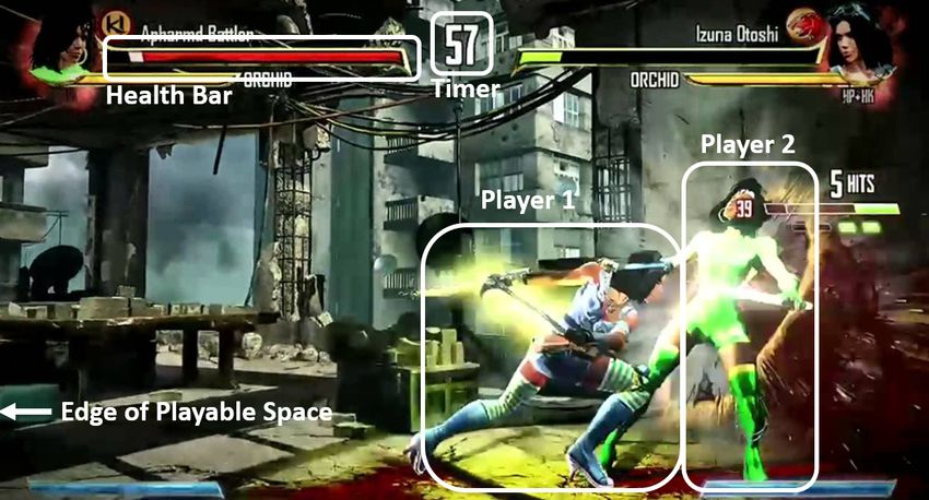
Application of Retrograde Analysis to Fighting Games

                      A Thesis

                    Presented to

    the Faculty of the Daniel Felix Ritchie School

       of Engineering and Computer Science

                University of Denver

                In Partial Fulfillment

         of the Requirements for the Degree

                  Master of Science

                         by

                     Kristen Yu

                      June 2019

            Advisor: Nathan Sturtevant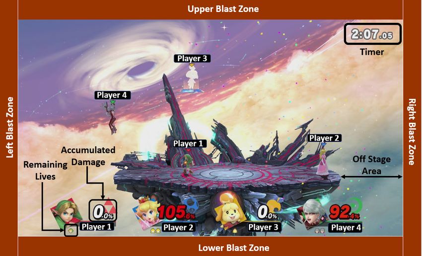
©Copyright by Kristen Yu 2019

     All Rights Reserved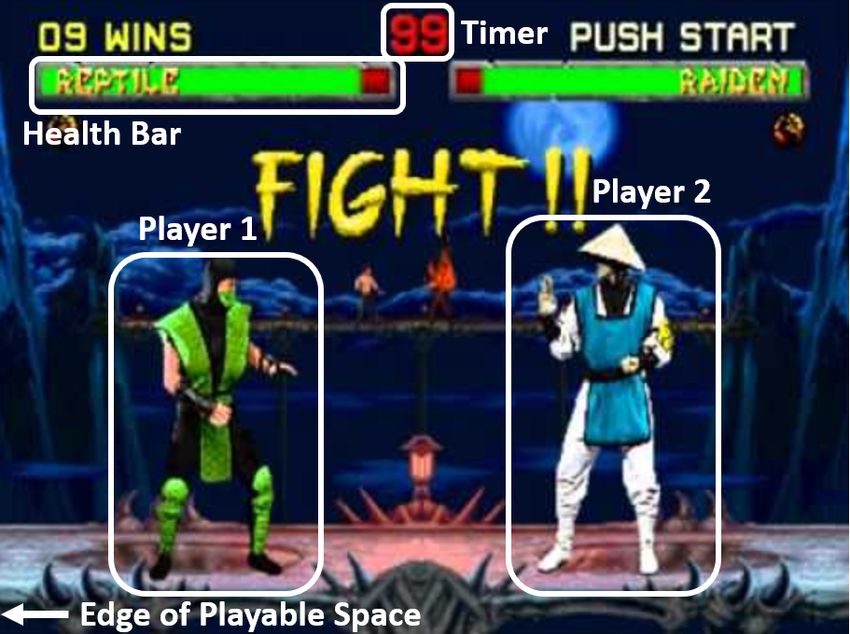
Author: Kristen Yu
Title: Application of Retrograde Analysis to Fighting Games
Advisor: Nathan Sturtevant
Degree Date: June 2019

                                      Abstract

    With the advent of the fighting game AI competition [34], there has been re-
cent interest in two-player fighting games. Monte-Carlo Tree-Search approaches
currently dominate the competition, but it is unclear if this is the best approach for
all fighting games. In this thesis we study the design of two-player fighting games
and the consequences of the game design on the types of AI that should be used
for playing the game, as well as formally define the state space that fighting games
are based on. Additionally, we also characterize how AI can solve the game given
a simultaneous action game model, to understand the characteristics of the solved
AI and the impact it has on game design.

                                          ii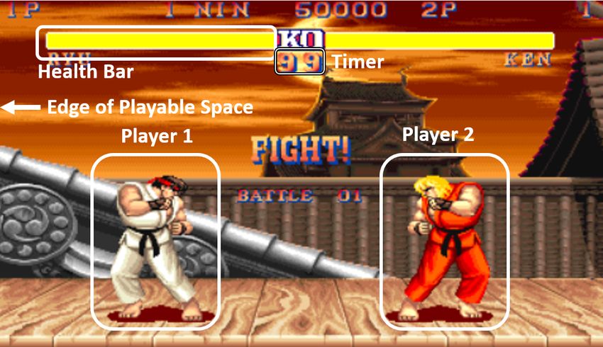
Acknowledgements

    First, I would like to thank Dr. Nathan Sturtevant, for his advice, guidance,
and for pushing me just enough so that this thesis would actually get done. Sec-
ond, I would like to thank Matt, Tram, and Chad for continuously supporting me
no matter how far I move away.

                                       iii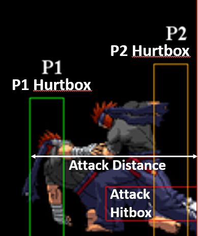
Table of Contents

1 Introduction                                                                                                                               1
  1.1 A History of Games and AI . . . . . .                           .   .   .   .   .   .   .   .   .   .   .   .   .   .   .   .   .   . 1
  1.2 Techniques for Fighting Games . . . .                           .   .   .   .   .   .   .   .   .   .   .   .   .   .   .   .   .   . 4
       1.2.1 Street Fighter 2: World Warrior                          .   .   .   .   .   .   .   .   .   .   .   .   .   .   .   .   .   . 5
       1.2.2 Mortal Kombat 2 . . . . . . . .                          .   .   .   .   .   .   .   .   .   .   .   .   .   .   .   .   .   . 7
       1.2.3 Skullgirls . . . . . . . . . . . . .                     .   .   .   .   .   .   .   .   .   .   .   .   .   .   .   .   .   . 8
       1.2.4 Super Smash Bros . . . . . . . .                         .   .   .   .   .   .   .   .   .   .   .   .   .   .   .   .   .   . 9
       1.2.5 Killer Instinct . . . . . . . . . .                      .   .   .   .   .   .   .   .   .   .   .   .   .   .   .   .   .   . 11
  1.3 Related Work . . . . . . . . . . . . . . .                      .   .   .   .   .   .   .   .   .   .   .   .   .   .   .   .   .   . 13
  1.4 Thesis Overview . . . . . . . . . . . . .                       .   .   .   .   .   .   .   .   .   .   .   .   .   .   .   .   .   . 15

2 Fighting Games                                                                                                                              16
  2.1 Fighting Game Design        .   .   .   .   .   .   .   .   .   .   .   .   .   .   .   .   .   .   .   .   .   .   .   .   .   .   .   16
  2.2 Game Play Mechanics .       .   .   .   .   .   .   .   .   .   .   .   .   .   .   .   .   .   .   .   .   .   .   .   .   .   .   .   17
  2.3 Game Play Dynamics .        .   .   .   .   .   .   .   .   .   .   .   .   .   .   .   .   .   .   .   .   .   .   .   .   .   .   .   19
  2.4 Game Balance . . . . .      .   .   .   .   .   .   .   .   .   .   .   .   .   .   .   .   .   .   .   .   .   .   .   .   .   .   .   24

3 Solving a Fighting Game                                                                                                                     26
  3.1 Solving a Fighting Game         .   .   .   .   .   .   .   .   .   .   .   .   .   .   .   .   .   .   .   .   .   .   .   .   .   .   26
       3.1.1 Rumble Fish . . .        .   .   .   .   .   .   .   .   .   .   .   .   .   .   .   .   .   .   .   .   .   .   .   .   .   .   27
  3.2 Retrograde Analysis . .         .   .   .   .   .   .   .   .   .   .   .   .   .   .   .   .   .   .   .   .   .   .   .   .   .   .   29
       3.2.1 Discounting . . .        .   .   .   .   .   .   .   .   .   .   .   .   .   .   .   .   .   .   .   .   .   .   .   .   .   .   31
       3.2.2 Epsilon Greedy .         .   .   .   .   .   .   .   .   .   .   .   .   .   .   .   .   .   .   .   .   .   .   .   .   .   .   33

4 Results and Discussion                                                             34
  4.1 Analysis of Strategies . . . . . . . . . . . . . . . . . . . . . . . . . . . . 38

5 Custom Fighting Game                                                                                                                        40
  5.1 Custom Game Design . . . . . . . . . . . .                              .   .   .   .   .   .   .   .   .   .   .   .   .   .   .   .   40
  5.2 Results of Custom Game . . . . . . . . . .                              .   .   .   .   .   .   .   .   .   .   .   .   .   .   .   .   42
  5.3 Modifications to the Custom Game . . . .                                .   .   .   .   .   .   .   .   .   .   .   .   .   .   .   .   45
  5.4 Results from the Modified Custom Game                                   .   .   .   .   .   .   .   .   .   .   .   .   .   .   .   .   46

6 Conclusion and Future Work                                                         48
  6.1 Conclusion . . . . . . . . . . . . . . . . . . . . . . . . . . . . . . . . . . 48
  6.2 Future Work . . . . . . . . . . . . . . . . . . . . . . . . . . . . . . . . . 48

                                                  iv
List of Figures
1 Introduction
1.1 Example of a Decision Tree for a Fighting game AI . . . . . . . . . . . 5
1.2 Screen Shot of Street Fighter 2: World Warrior . . . . . . . . . . . . . . 6
1.3 Screen Shot of Mortal Kombat 2 . . . . . . . . . . . . . . . . . . . . . . 8
1.4 Screen Shot of Skullgirls . . . . . . . . . . . . . . . . . . . . . . . . . . 9
1.5 Screen Shot Super Smash Bros Ultimate . . . . . . . . . . . . . . . . . 11
1.6 Screen Shot of Killer Instinct (2013) . . . . . . . . . . . . . . . . . . . . 12
2 Fighting Games
2.1 Illustration of the spacing distances for an attack . . . . . . . . . . . . 17
2.2 FSA that governs the players actions . . . . . . . . . . . . . . . . . . . 18
2.3 Information set created by the simultaneous move model . . . . . . . 20
2.4 Reward matrix for Player 1 in rock paper scissors . . . . . . . . . . . . 21
2.5 Effectiveness of moves A, B, and Block in relation to each other . . . . 22
2.6 Illustration of reward being propagated through time . . . . . . . . . 24
3 Solving a Fighting Game
3.1 Retrograde Analysis . . . . . . . . . . . . . . . . . . . . . . . . . . . . 31
4 Results and Discussion
4.1 Results from the Baseline Nash AI . . . . . . . . . . . . . . . . . . . . 35
4.2 Results from the Discount AI . . . . . . . . . . . . . . . . . . . . . . . 36
4.3 Results from the Epsilon AI . . . . . . . . . . . . . . . . . . . . . . . . 37
4.4 Percentage of mixed strategy moves . . . . . . . . . . . . . . . . . . . 38
5 Custom Fighting Game
5.1 Effectiveness wheels for close distance . . . . . . . . . . . . . . . . . . 42
5.2 Effectiveness wheels for far distance . . . . . . . . . . . . . . . . . . . 43
5.3 Results from the Custom Game . . . . . . . . . . . . . . . . . . . . . . 44
5.4 Updated Effectiveness wheel for the close distance . . . . . . . . . . . 46
5.5 Updated Effectiveness wheel for the far distance . . . . . . . . . . . . 46
5.6 Results from the Modified Custom Game . . . . . . . . . . . . . . . . 47
vAbbreviations
AI Artificial Intelligence
FSM Finite State Machine
RPS Rock Paper Scissors
vi1 Introduction
1.1 A History of Games and AI
This thesis studies the problem of fighting game AI. In this space there are a
few areas of interest that can be addressed, such as creating an AI that will beat
any human or computer opponent, creating an AI that is interesting for humans to
play against, and scaling the skill of an AI with the skill of a player. Recent work
in Fighting Game AI has focused on building strong AI players [1-12] which will
beat any opponent, and the current competition has a component which focuses on
how to beat opponents as quickly as possible [34]. This raises the question of what
it would mean to solve a fighting game, or to build a perfect fighting game AI. The
definition of a perfect player depends critically on the definition of the game being
played. However, current literature, to our knowledge, does not contain a precise
definition of a fighting game, meaning that the notion of building a perfect AI for
such games is ill-defined.
Thus, the focus of this thesis is threefold. First, the paper builds a broad defi-
nition of the state space of a fighting game based on the cross product of finite state
machines that determine the possible actions for each player at each stage of the
game. Because players have the potential to take actions simultaneously, there are
then information sets defined over these states. Next, the paper shows how a game
1can be solved via retrograde analysis and using Nash equilibria to determine op-
timal play over the information sets. Finally, the paper builds an optimal strategy
for a small fighting AI game and characterizes the solution to the game. Even in
a simple game the optimal strategy is complex enough to be non-trivial, such that
simple strategies will not perform well against the optimal AI. This work opens
the door for deeper study of both optimal and suboptimal play, as well as options
related to game design, where the impact of design choices in a game can be stud-
ied. We begin with a historical context of work in game AI as well as specific work
in fighting games.
Games have a long history of being used as a training ground for AI, either
as applications of new ideas or for the design of new algorithms. One of the first
games that was studied was chess. Alan Turing in 1948 wrote a program that could
play chess [42]. Bellman also did early work in AI and chess, designing algorithms
using dynamic programming in 1965 [32]. During the 1960’s work was also being
done with single player games such as sliding tile puzzle and towers of Hanoi be-
cause they were simpler problems to solve [43,44]. Agents that play these single
player games have unlimited time to make a decision, and can do preprocessing
in order to understand the entire state space that these puzzles have, while mul-
tiplayer games have to account for opponent decisions. Thus, these are entirely
different problems to solve and require different algorithms to solve. Chess and
checkers can be bench-marked against humans, which allows for the effectiveness
of the algorithms used to be measured. Some of these agents were able to become
better than human players, with IBM’s Deep Blue beating a chess grand master in
1997 [45], and Schaeffer’s Chinook officially solving checkers in 2007 by showing
that the game always results in a draw with perfect play [46].
2From there, AI research began to transition to playing more and more difficult
games. These games have state spaces that are exponentially large, so they cannot
be explored using traditional algorithms such as minimax or alpha-beta search.
Because of this, reinforcement learning or neural networks are often deployed to
solve these problems. In recent times IBM’s Watson was able to beat expert jeop-
ardy players in 2011 [47], and Google’s AlphaGo bested the world champion of Go
in 2017 [48]. Heads-up limit Texas Hold’em poker was solved by Bowling et al in
2015 [40], and the AI DeepStack designed by the same research group was able to
beat professional players in no-limit Texas Hold’em poker in 2017 [41].
Video games can also provide a variety interesting problems to solve due to
the complexity of their rules. In 2009, an A* agent designed by Baumgarten won a
competition for playing the longest level of infinite Mario, based off of Super Mario
World [50]. Google’s DeepMind bested the top Starcraft II players [51], which is a
complex real time strategy game with resource management and combat aspects,
and Elon Musk’s Open AI beat a team of esports champions at Dota 2, a multi-
player arena game in 2018 [52].
Fighting games are a genre of video games that has seen less research in the
academic community. A fighting game has 2 to 8 players fighting in a competitive
match where one player will become the victor. Fighting games differ from other
competitive multiplayer games such as first person shooters because their primary
game mechanic is centered around some form of martial arts, whether based on
a real fighting style or one created for the game. Fighting games as a genre are
popular in the esports arena, with the main interest in the game being competing
against other human players as opposed to the AI that exist within the game. This
3is due to a variety of problems, but is largely due to the fact that the AI are either
too easy or too hard.
The design of an AI then becomes a question of not only for the AI to play
the game but also of how difficult the AI is for a human player. The other aspect
of a fighting game AI would be whether the AI is interesting to play against for
a human - an AI that is hard to beat is not necessarily interesting to play against.
The challenge then becomes finding an AI that is balanced between difficulty and
interesting play, such that this will be true for any player skill level.
1.2 Techniques for Fighting Games
The Extra Credits Youtube channel, written by an industry veteran, states that
the main technique for building fighting game AI in industry is using decision
trees [49]. A decision tree consists of three types of nodes: decision nodes, chance
nodes, and leaf nodes. A decision node is a branch in the tree which represents
a specific choice that the AI can make. The children of this node are the possible
choices that the agent may select. Chance nodes represent the possible outcomes
of an event which the agent cannot choose, and all of the children of this node
represent the possible courses of action given this chance. A leaf node represents
a singular action that results from following any single path down the tree. Figure
1.1 shows an example of a simple decision tree that could be used for a fighting
game.
Each decision tree has to be specifically tailored to a character, and modified
for each difficulty available. This is extremely time and labor intensive, and even
4Is the opponent close?
Yes No
Is the opponent currently attacking? Did the opponent use a projectile?
Yes No Yes No
Chance node Strong attack Is the projectile close to me? Projectile
75% 25% Yes No
Counter attack Block Jump Move closer
F IGURE 1.1: Example of a Decision Tree for a Fighting game AI
models that seem simple take many resources to create. Despite these drawbacks
decision trees are still the dominant algorithm used to implement AI in fighting
games. The rest of this section will describe the AI used in various published
game.
1.2.1 Street Fighter 2: World Warrior
Street Fighter 2: World Warrior by Capcom was released in 1991 for arcade
cabinets. It is a classic fighting game, and is part of the franchise that initially
made this genre popular. In Figure 1.2, there is a screen shot of the game which
illustrates the important features of the game in white boxes, such as the player
health and the round timer. As with most classic fighting games, the goal is to
reduce the opponent’s health to zero before the time runs out. The AI used for
this game is a decision tree with small modifications. A fighting game enthusiast
deconstructed the compiled code to determine the decisions that some of the char-
acters use [35]. There are variables that determine which level the AI is playing at,
and other variables that directly influence the player actions. This decision tree has
5F IGURE 1.2: Screen Shot of Street Fighter 2: World Warrior
three main branches with which the AI can choose actions. The first is waiting for
an attack from the opponent, the second is actively attacking the opponent and the
third is reacting to an opponent attack. With these branches, the AI can choose be-
tween eight layers of possible options which are dependent on the amount of time
left in the round. This AI is allowed to execute moves differently than a human
player would have to, with the example of a charge attack. In Street Fighter, some
moves require that a certain button be pressed and held down for a small amount
of time in order for that move to be executed. The AI in this game can execute
these attacks without the required input time, which makes them react faster. This
AI also includes instructions such as “wait until I can attack”, which means that
the AI is able to execute frame-perfect moves. Frame-perfect refers to an action
that is executed at the optimal frame in time, in this case attacking immediately
as it is able to do so. If the game runs at 30 frames per second, then each frame
is 33ms. Since the AI has the ability to wait, then it can simply wait for a frame
where it registers that it is capable of attack, and then initiate that attack in that
same frame, or less than 33ms later.
61.2.2 Mortal Kombat 2
Mortal Kombat 2 was released in 1993 for arcade cabinets by the publisher
Midway. As shown in Figure 1.3, it is another example of a classic fighting game
that uses decision trees. This decision tree frequently uses the advantages that a
computer has over a human to win matches. The Youtube channel Unbreakable
was able to decode this decision tree by executing moves, and then record the
resulting AI behavior [36]. The main state of this AI is a react phase, where the AI
will simply choose the best counter to any move that its opponent inputs. Since the
AI has perfect knowledge of the game state, it knows the move that its opponent
chooses the frame that the move is executed, and then is able to respond in that
same frame. This kind of “super human” reaction speed is the main difficulty
adjustment for the AI in this game. These AI are also allowed to execute moves in
a sequence that human players cannot. Under normal circumstances, some moves
have a cool down period. A cool down period is a period time where a player
cannot execute any actions, regardless of whether a new action is input or not. For
the AI, this cool down period is eliminated, which allows it to cheat in the game
where a human player cannot. This AI also has a clear advantage over human
players in the effectiveness of their moves. If an opponent is crouching, a human
player cannot throw them. However, an AI is able to throw crouching opponents.
This is perhaps one of the most obvious way that the AI can cheat at any game.
7F IGURE 1.3: Screen Shot of Mortal Kombat 2
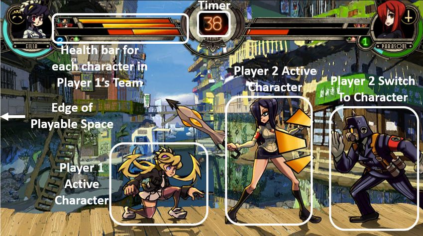
1.2.3 Skullgirls
Skullgirls, shown in Figure 1.4, was originally released in 2012 on PlayStation
Network, Xbox Live Arcade, and Steam and has since been expanded to several
other platforms, such as mobile. This game was developed by Reverge Labs and
published by Marvelous and Autumn Games. The lead programmer of this game
is a fighting game tournament veteran, and his main goal in creating this game
was to take the classing fighting game model and balance the game such that it is
suitable for esports level competition. In this game, a player is allowed to create a
team of characters and freely switch between those characters as long as they have
health, which helps combat character imbalances. Ian Cox, one of the developers
and the man in charge of AI design, wanted to create AI that is both satisfying to
play against and instructional for new players [38]. Their decision trees were de-
signed to incorporate particular strategies such as “anti-air”. These strategies are
8F IGURE 1.4: Screen Shot of Skullgirls
hand-crafted policies, which are intentionally predictable to allow for humans to
learn that particular strategy. In addition to difficulty variants, each AI is specif-
ically modified to play against every character in the game, in order to take ad-
vantage of each character’s strengths and weaknesses. This is done in an effort to
encourage the player to learn particular skills. For example, if the player chooses
a character whose best move is a throw, then the opponent will intentionally play
using a strategy that is vulnerable to throws. Skullgirls is one of the published
fighting games available that consciously chooses to have their AI be an integral
mechanic to learning how to play the game, instead of the goal of the AI to just be
to beat the opponent.
1.2.4 Super Smash Bros
Super Smash Bros Brawl and Super Smash Bros Ultimate are two games pub-
lished by Nintendo as part of their Super Smash Bros franchise. Brawl was released
9on the WiiU in 2014 and Ultimate was released on the Switch in 2018. These fight-
ing games are unique because they do not follow the classic fighting game model.
Instead of health, the fighters in the game have a percentage ranging from 0 to
999 that is representative of the amount of damage they have accumulated in the
game, and a finite amount of lives ranging from 1 to 99. The goal of the game
is to force the characters off the stage, and into areas called “blast zones”. These
blast zones are located on the upper, lower, right, and left hand side of the screen,
shown in Figure 1.5. When one player enters a blast zone, they lose a life. The
winner of the match is either the player with the most amount of lives when the
timer runs out, or the only remaining player with lives. There is a toy that can be
trained to play the game called an Amiibo, which implements some sort of learn-
ing algorithm based on observing human play. These Amiibo start at level 1, and
work their way to level 50, learning to play the game as their level progresses.
Unlike some other games, the hardware that powers these Amiibo has not been
cracked so there is no compiled code to dissect. However, there has been extensive
testing for the capabilities of the AI and there are some emerging theories on the
algorithms that are used in these Amiibo. According to discussions on reddit, the
Amiibo themselves have an underlying decision tree which governs specific be-
haviors that would want to be executed under all circumstances, and a learnable
section where the AI will learn to favor specific moves over other moves [37]. For
example, as shown in Figure 1.5, there is an offstage area where a character is in
danger of falling to its death. A dedicated behavior that would be necessary for
any AI would be for that AI to jump back to the stage to avoid dying. This has
been demonstrated with many tests to determine that this behavior is not affected
10F IGURE 1.5: Screen Shot Super Smash Bros Ultimate
by the training that each individual Amiibo receive. What does appear to be af-
fected is the frequency of the moves which are executed by that Amiibo. These
Amiibo will learn a distribution of moves to be executed, but none of these moves
can be learned such that a single move is never executed. These Amiibo AI also
cannot learn to execute moves in succession, which further supports the idea that
the learning part of their algorithm is simply adjusting the frequency with which
particular actions are chosen.
1.2.5 Killer Instinct
The Killer Instinct reboot in 2013 is also a conventional fighting game, as
shown in Figure 1.6, but they shipped it with two different kinds of AI. The first be-
ing decision based AI similar to ones that have previously been discussed, and the
second being “shadow AI”. These shadow AI are perhaps the most complicated
11attempt of creating an interesting agent for humans to play against, and are capa-
ble of being trained to play the game by replicating specific patterns that a player
would use. According to the Youtube Channel “AI and Games”, the AI records
all of the opponent play data, and then attempts to match the individual moves to
high level mechanics in order to learn complicated behavior such as combos [39].
The Shadow AI uses case-based reasoning to build models based off of the col-
lected data, which more closely mimics how humans base their strategy decisions
based off of previous experience [53]. This system is also unique due to its capac-
ity to learn weaknesses in specific characters. While the Nintendo Amiibo exhibits
more human-like behavior than purely decision based AI, it lacks the ability to
learn policies tailored to a specific character.
F IGURE 1.6: Screen Shot of Killer Instinct (2013)
There are also many AI and fighting game enthusiasts building toy AI for their
own personal projects. They are generally built using neural networks, likely due
to the high availability of packages such as PyTorch and Keras that facilitate the
creation and training of these AI. These kinds of AI are seeing some success when
12played in their respective games, but there is often little to no bench-marking so
the true capability of these AI is unknown.
1.3 Related Work
In academia, there are several algorithm classes that have been implemented
on fighting game platforms in order to design fighting game AI. At the Confer-
ence on Games, there is an annual competition hosted by Ritsumeikan University
using a platform called Fighting ICE [34]. In this competition, the AI is playing
a fast-paced game where it has a reaction speed of 15 frames at 60 frames per
second, and is playing other AI using different strategies to determine a winner
with a round-robin tournament. Early work attempted to improve on the existing
rule-based AI that are common in published games by implementing a prediction
algorithm, K-Nearest Neighbors [1,2,3,4]. These predictions assumed that there is
one dominant move at every state in the state space, and aim to predict that sin-
gle move. Hierarchical Task Networks were also added to the existing rule-based
AI as a way of implementing prediction, but was unable to plan effectively [25].
This work was abandoned in favor of Monte Carlo Tree Search (MCTS) algorithms
which have consistently placed in the top 3 for the competition [5,6,7,8,9,10]. As
such, there has been other research to improve this model by combining it with
existing algorithms. Genetic algorithms [11], Action tables [12], and Hierarchical
Reinforcement Learning [13] have all been combined with MCTS in attempts to
improve on the original algorithm. MCTS works by searching a tree for a set pe-
riod of time, and returning either the correct answer or the best answer found so
far. This algorithm has been validated experimentally to perform well through
13competing against other AI, but there has been no published work to understand
why this algorithm is effective. MCTS will continually reach its time limit without
finding a true optimal move, and is only finding locally optimal moves because
there is not enough time to search the state space. In this case, the locally optimal
move is usually some sort of kick, which means that the AI is usually choosing to
do damage in most states, and is therefore performing well within the competition.
Another type of algorithm that has been implemented is a multi-policy one,
where the rules of the agent are designed to be switched based off of the state pa-
rameters [16,17]. These types of algorithms rely on dynamic scripting [23,24] to
learn the optimal state with which to execute each individual policy. More compli-
cated algorithms such as genetic algorithms [19], neural networks [20,21,22], and
hierarchical reward architecture [26] have all been implemented on the fighting
ICE framework and have learned strategies that are stronger than the “default"
rule based AI.
Other research beyond the competition has been done using AI-TEM frame-
work, which is a Game Boy Emulator that can play a variety of games. The AI
reads the components of the chosen fighting game in order to make informed de-
cisions. An agent was trained by learning how a human would play a game [14],
in an attempt to learn a viable strategy. A neural network was also trained using
human play data [15] on a different game, or the human play data was used to
create a FSM that plays similar to a rule based AI.
141.4 Thesis Overview
In Chapter 2 we discuss the required features of fighting game design, and
analyze the mechanical impact of each design choice. The mechanics of the game
then can be evaluated based on a mechanics-dynamics-aesthetics approach. A
fighting game can be modeled as simultaneous move game, which can then be
interpreted as a matrix game. These games can be solved to create a Nash Equilib-
rium, which is an optimal policy to play the game.
In Chapter 3 we discuss the fighting game that will be solved, Rumble Fish,
and discuss the main algorithm that will be used to solve the fighting game: retro-
grade analysis. A few variations on this algorithm are also implemented to model
imperfect behavior and to encourage different play styles from the Nash Equilib-
rium player.
In Chapter 4 we solve the fighting game using retrograde analysis. This cre-
ates a Nash Equilibrium solution and that agent is evaluated against a few simple
strategies in order to characterize the solution.
In Chapter 5 we create a custom fighting game based on a new understanding
of the impact that game design has on the Nash Equilibrium solution. This custom
game is also solved using retrograde analysis, and the results evaluated against
simple strategies to characterize the Nash Equilibrium player.
Chapter 6 is the conclusion and future work for this research topic.
152 Fighting Games
2.1 Fighting Game Design
In its simplest form, all fighting games have these three basic design elements:
Timing, Spacing, and Effectiveness. Each of these design elements are parame-
terized to make up the overall design of the game.
• Timing is the duration attributed to the actions that can be executed in the
game. This is split into a few categories: lead time, attack duration, lag time,
and input time. The input time is the amount of time required for a player to
input a move, which is generally shorter than the other timings. Lead time is
the time before the attack is executed. The attack duration is the amount of
time that an attack has damaging potential. Lag time is the amount of time
after a move has been executed that a player is unable to input another move.
• Spacing is the distances that are important in the game. Both moves and
characters have spacing. Each character has two different dimensions that
are important: the hurtbox and the hitbox [54]. The hurtbox is the area that
the opponent can attack without taking damage, and the hit box is the area
during an attack that can inflict damage to the opponent, shown in Figure
2.1. Move spacing can be split into two categories: The distance in which
a particular action will hit an opposing character, and the area of its hitbox.
16F IGURE 2.1: Illustration of the spacing distances for an attack
Similarly, the character spacing can be split into the area of its hurtbox and
it’s individual x and y coordinates.
• Effectiveness is the performance of a given action. Usually this is the amount
of damage assigned to an action, but it can also be affected by its relation to
other moves. Suppose there is a block mechanic in the game. If player one
blocks and player two attacks, player two’s move can be partially or fully
blocked, which decreases the effectiveness of the move.
2.2 Game Play Mechanics
This paper will analyze the mechanics and dynamics from a Mechanics-
Dynamics-Aesthetics (MDA) perspective [31]. Any fighting Game can be mod-
eled by a Finite State Machine (FSM) which determines the outcomes of a players
controls for a given state. Each FSM f has a time t associated with it, and list of
available actions that the agent can take m1 ...mk , where k is finite. This FSM has a
17F IGURE 2.2: FSA that governs the players actions
starting state s0 where the player is idle, as shown in Figure 2.2. When a player se-
lects an action mi , i ∈ {1...k }, the state of the machine transitions to the start of the
chosen move, with a lead time of tlead , continues to the action which has an attack
duration of t a , and ends with lag time tlag before returning to idle. Because of how
the FSM transitions, once the player has chosen a move, that move typically must
be executed to completion before another move can be attempted.
Each player has an individual FSM that is controlling the state in which that
player exists. By combining the two FSM, we can reach a state s g ∈ FSMP1 ×
FSMP2 . For the full state of the game, s g also has attributes a1 ...an , n ∈ N, of the
current state such as the health and the spacing of the individual players. These
attributes provide information about how to transition to the next state, such as
indicating whether an action does damage, and how much damage is assigned to
a player. The state s g transitions to the next state s0g through both the action of
player one and the action of player 2. This transition is deterministic and results in
a unique time, location, and states for each attribute, which is determined by the
outcome of the interaction of the actions that each player used. If player one suc-
cessfully attacks player two while player two is not at an idle state, then the FSM
for player two will automatically either transition to idle or to lag time, preventing
it from executing the remaining part of the machine.
182.3 Game Play Dynamics
Assume both player one and player two have one attack, m1 , with lead time
tlead = k1 , and their spacing is such that if either player executes the move, they
will do damage to their opponent. If player one is in the idle state and player two
chooses to execute m1 , then the attack m1 will be successful and player one will
take damage. If both players are in idle, the player that executes m1 first will do
damage. In this situation, whichever player can execute the action first will win.
However, fighting games usually have more than one move, with a variety of
lead times. Assume that player one and player two both have action m1 , but now
also have action m2 with lead time tlead = k2 , where k1 < k2 . If player one were to
execute m2 , then there is a period of time, k2 − k1 , where player two can execute
m1 and counter m2 . Using this model, the agent would simply have to wait for the
opponent to select a move, and then respond accordingly.
To simplify the game dynamics, assume that the FSM has no lead or lag time,
so that there is a single state with which the FSM can transition to from idle. Ad-
ditionally, restrict the timing of the game such that each player has to execute the
game, so then it becomes purely a simultaneous move game. This can be modeled
as Rock Paper Scissors (RPS) because it shares the quality of what fighting game
expert David Sirlin calls "double-blind decisions" [28]. Double-blind decisions are
created in a situation where both players are making a decision at the same time,
and both of their decisions are revealed at the same time. Double-blind decisions,
19Sirlin argues, fully capture the essence of fighting games because at the moment a
player chooses a move, they do not know exactly what the opponent is doing due
to the fast-paced nature of the game. The opponent’s move can be modeled using
information sets. An information set is the set of all the states that cannot be dis-
tinguished by a player because the state of its opponent is unknown, and a player
must make the same action in every state in an information set. Figure 2.3 shows
a game play tree which creates an information set. The root is the state of player
one, and the edges are the different actions available to player one, punch, kick, or
idle, which can be taken from that state. Each of the children of the root represent
the state of player two, where player two can also execute actions punch, kick, or
idle at that state. Once both players have selected a move, a reward is assigned at
each leaf, and the reward is dependent on both the action from player one and the
action from player two. The information set is the set of all nodes at depth one,
and is outlined by the box in the figure.
F IGURE 2.3: Information set created by the simultaneous move model
Besides information sets in an extensive-form tree, a simultaneous move game
can also be modeled as a matrix game which maps the n actions { a1 , a2 , ..., an }
20of each individual players to their rewards ri . Each player has its own reward
matrix M = n × n, which gives the instantaneous reward rij of player one taking
action i and player two taking action j at Mij . The payoff of for a given player Rk ,
k ∈ {1, 2}, is the total instantaneous reward accumulated by playing strategy some
strategy. The optimal policy π1 of player one is a policy that maximizes the payoff
of player one given all possible player two strategies. However, player two also
has an optimal policy it is trying to execute, so player one wants to minimize the
reward that player two gains simultaneously. Thus the optimal policy for player
one can be defined as max R1 min R2 ∑ rij . RPS can be modeled as a matrix game
M1 by assigning values to the outcomes of player one, as show in Figure 3. If the
result of an action is a win, 1 is assigned. If the result of an action is a loss then -1 is
assigned. If the result of an action is a tie then 0 is assigned. If the reward assigned
for some set of actions ai and a j for player two is the negative value of the reward
of the reward assigned for the same set for player one, then it is a zero sum matrix
game. In that case, the reward matrix for player two is M2 = − M1 .
P2 P2 P2
Rock Paper Scissors
P1
0 -1 1
Rock
P1
1 0 -1
Paper
P1
-1 1 0
Scissors
F IGURE 2.4: Reward matrix for Player 1 in rock paper scissors
By replacing the moves of RPS with moves from a fighting game, a similar
reward matrix can be generated. Let move a and move b be attacking moves,
21F IGURE 2.5: Effectiveness of moves A, B, and Block in relation to each
other
which have different effectiveness based on the opponent’s move. Move a will
inflict damage against a block, but not against move b. Move b will not inflict
damage against a block, but will against move a. Figure 4 shows the relationship
between these moves, where the arrow pointing 2.5 to another move indicates that
the move will "win" and inflict damage against that move.
Consider a game in which each player only selects one action, and the out-
come of the game is determined by effectiveness of the chosen moves in relation
to each other. Then the factors that influence whether a player wins are the spac-
ing between the two players and the effectiveness of the move. If the spacing is
such that the two players are out of attack distance, then, the entire reward ma-
trix would be zero. However, if the spacing between the two players is such that
they are within attack distance of each other, then the moves have the possibility of
doing damage and generating an interesting reward matrix. The diagonal of this
matrix is zero because both players would successfully execute the move, in which
case the reward would be 1 + -1 = 0.
22A given payoff matrix can be solved using linear programming which finds
the policies π1 and π2 , for player one and player two respectively. These poli-
cies are the set of probabilities with which each move in the game should be used,
which forms the strategy for each player. An optimal strategy for a player is one
that maximizes its own payoff and minimizes its opponent payoff. In practice, this
means that the player cannot unilaterally change their policy to gain more reward,
provided that their opponent does not change their strategy. If both players are
playing with their optimal policies, it is a Nash Equilibrium. Using the rock paper
scissors analogy, if both players are attempting to play optimally, the optimal strat-
egy for player one is to use each move 1/3 of the time, and the optimal strategy for
player two is to use each move 1/3 of the time.
Timing still needs to be considered in the fighting game model. Time is not
infinite, because there is a time limit imposed on the game itself. Thus, there are
two ending conditions for a match, when the timer reaches zero or if one of the
player’s health becomes 0. If the player’s health becomes 0, we can introduce a
higher reward value for that move, which incentivizes the agent to win the game.
For every state s, each time step has its own reward matrix, and the individual
reward matrices for each state are linked through time. The time in which that
state has a higher reward has an effect on the future reward matrices, because that
high reward is propagated through all future times, as show in Figure 2.6. The
value in red at time 0 is the initially high reward, and gets propagated to time 1.
At the final reward matrix at time t, the final reward is still affected by the initial
high reward.The rewards in the matrix are then influenced both by the positions
of the players, and the rewards of the previous matrices.
23F IGURE 2.6: Illustration of reward being propagated through time
2.4 Game Balance
Balancing the game is adjusting the different game play mechanics such that
they interact in a way that produces the desired outcomes. For fighting games,
usually the goal is to prevent a dominant character or strategy from appearing. A
dominant strategy is a policy that wins against any other policy that its opponent
chooses. A dominant strategy can be difficult to prevent because there is an inher-
ent level of uncertainty integrated into the gameplay mechanics. While a player
is playing the game, they do not know which move the opponent will pick next,
which makes the player have to predict what the opponent’s move will be. Sirlin
describes the ability to predict the opponent’s next move as "Yomi" [28,29]. When
the opponent’s move is uncertain, the player engages in Yomi because they are
forced to make their best guess on what move the opponent will make, and then
respond appropriately given that prediction. Sirlin argues that using a rock paper
scissors like mechanic for the core of action resolution is the optimal way to bal-
ance fighting games, because it forces Yomi interactions and prevents any single
move from becoming dominant.
24Aside from properly balancing the individual game mechanics, fighting games
also need to balance the level of skill. Each move is assigned a certain number of
inputs that the player must make in the correct order in order to execute that move.
These can be simple - such as simply pressing the A button - to extremely complex
- such as quarter circle right, quarter circle right, A button, B button. This skill af-
fects the game play because a higher difficulty level would create a higher chance
of the human incorrectly inputting the move, which would trigger a random move
being executed. A computer has the ability to correctly input any move at any
state, while a human will always have some probability of incorrectly inputting
any move.
253 Solving a Fighting Game
3.1 Solving a Fighting Game
An analysis of how MCTS performs in RPS by Shafiei et al [33] demonstrated
that it produces suboptimal play because it cannot randomize correctly for a RPS
type of game play model. In a simultaneous move fighting game, the time limit
ending condition allows for retrograde analysis to be used to work backwards
from the end of the game to the start state. Bellman showed that this technique
can be applied to chess and checkers [32] using minimax trees where the max or
the min is taken at each state and propagated through the tree. With imperfect in-
formation at each state, we instead compute the Nash Equilibrium at each state and
propagate the expected value of the Nash Equilibrium. This approach is based on
work done by Littman and Hu, which applied reinforcement learning algorithms
to markov games to create a nash equillibrium [36,37].
Using retrograde analysis allows for a quick convergence of the state space.
In a fighting game, the end of the match is when when one player’s health reaches
zero, or when the timer runs out. Neither player can change the outcome of the
game by inputting new moves. Thus, the ending states of a fighting game are
always correct, so when the values are propagated backward it has a correct start-
ing point. If forward passes were used, incorrect values would have to be passed
26to the next iteration, until that system converges, which is more computationally
expensive.
The solution to the fighting game found using the retrograde analysis is the
optimal policy for each player to use at each state of the game. These information
sets that appear as matrix games for each state in the retrograde analysis can be
solved using linear programming to find the optimal policy and create a Nash
Equilibrium.
3.1.1 Rumble Fish
The fighting game chosen for the computational model is a game called Rum-
ble Fish. Rumble Fish is similar to Street Fighter, and is also the game that is used
in the Fighting ICE competition. It takes in eight directional inputs and two but-
tons, which can be executed in sequence to produce moves. These moves can then
be strung together into combos to deal more damage. While playing, the char-
acter can build up mana, which allows them to execute stronger moves such as
projectiles that cost mana.
We simplified the game in several ways to solve the game quickly and under-
stand the impact of the game and solver design on the optimal strategy. Only one
character was chosen, so that the same character would be playing against itself.
This was to eliminate differences between characters, where one character could
have actions that dominate other characters. This could always win the game. The
width of the game play screen was also reduced, and the jumping and mana me-
chanics were eliminated. Only five moves were chosen to begin with:
27• Move Forward: Move towards the other player by 25 pixels
• Move Backward: Move away from the other player by 120 pixels
• Punch: A short range attack with a damage of 5
• Kick: A long range attack with a damage of 10
• Block: A block will only affect the kick, which reduces the given damage to
0. The block is ineffective against punches and the player will still take 5
damage when punched
The block was further modified to introduce an RPS mechanic. Originally, the
block will block all moves in the game, resulting in the blocking player to take
only a fraction of the damage. This causes the kick to become the dominating
action because it has the longest reach and the highest damage. Instead, the block
is modified such that it is only effective against the kick, and a successful block
will reduce all damage to zero. The initial health was also set to be 20, and all
distances between 0 and 170 pixels were examined. The maximum distance of 170
was chosen because the kick has a range of 140 pixels. All distances larger than
170 are treated as the state 170 because if the players are out of attack distance and
moving forward does not bring you into attack range, it can be treated in the same
way. If a punch or a kick is successful, the opposing player will be pushed back.
However, if the opposing player was blocking then they will not move. The length
of the game was not fixed, but the retrograde procedure in the next section was
run backwards until the policy converged.
283.2 Retrograde Analysis
Retrograde analysis is more efficient than forward search for this state space.
Time starts at the end of the match, and then runs backwards to the start of the
match. The flow through for this algorithm is shown in Figure 3.1. Moves Forward
Walk, Back Step, Punch, Kick, and Block have been abbreviated "fw", "bs", "p", "k",
and "b" respectively. This figure shows the payoff matrix for any given state s,
where the values at each index i, j is the value of the state at the previous time
step when actions ai and a j are chosen. When the time is zero, the box on the left
indicates the the value of the state is the difference in health for player 1 and player
2. When the time is not zero, the value of the state is calculated differently. The first
down arrow shows that the policy for player one is determined, which is then used
to find the expected value of that state. This new state value then feeds back into
the payoff matrix for the next state. A more precise description of the approach is
described below.
Each time step t is one frame backwards in time and the analysis is run un-
til the beginning of the match is reached. At time t = 0, the value v0 (s) of each
state s ∈ S was initialized to be the difference in health from player one to player
two. Each possible health value for player one and player two were considered,
to account for the situation where time runs out. If the state s was a winning state
for player one, meaning that player two’s health is zero and player one’s health
is nonzero, then the value of the state was increased by 100 because those are the
most desirable states for player one to be in.
29The reward for losing is not decreased by 100, in order to encourage the agent
to continue attacking even if it is at low health.
To calculate the value of state s at time t > 0, a 5x5 reward matrix is created
where player one is represented by the rows and player two is represented by the
columns. All of the rewards assigned to each outcome is the reward for player
one. The rewards for player two are the negative value of each reward, which
can be calculated without creating another matrix. Given a set of five actions A =
{Forward Walk, Back Step, Punch, Kick, Block}, each row i and each column j is a
selection a ∈ A, where ai is the action for player one and a j is the action for player
two. The next state s0 is the state reached by executing actions ai and a j at state
s. The intersection i x j is the reward of the moves ai and a j that were chosen at
state s, which is the value of the state vt−1 (s0 ) . This matrix is then solved using
linear programming to produce π1 and π2 , which are the policies of player one
and player two. Each policy represents the probabilities that each action in a ∈ A
should be executed for state s at Nash Equilibrium. The value of state s is the
expected value of that state calculated as follows:
5 5
vt (s) = ∑ ∑ p a i p a j v t −1 ( s 0 ) (3.1)
i =1 j =1
This value vt (s) is stored for the time t. When two actions lead to s at time
t + 1, the value vt (s) is used as the reward for those actions. In this way, the
state values will propagate through the time steps to produce the final state. The
iteration process is monitored for convergence for all states s using a δ, where
δ = Vt (s) − Vt−1 (s). When δ < 0.01, the values are considered converged.
30F IGURE 3.1: Retrograde Analysis
The flow through for the modified retrograde analysis algorithm when applied to
fighting games
3.2.1 Discounting
The basic retrograde analysis has no preference for winning a game earlier or
later in a game, but discounting can be applied to the reward function in order to
encourage the agent to prefer winning earlier. This can be done by discounting the
future reward, so that the current or immediate reward Ri has a larger impact on
the overall value of the state. The value of a state is given as follows:
vt (s) = Ri + discount ∗ vt (s0 ) (3.2)
5 5
0
vt (s ) = ∑ ∑ pai paj vt−1 (s00 ) (3.3)
i =1 j =1
31where s0 is the next state and s00 is the state after the next state.
The immediate reward function was defined as followed:
• Move Forward: -1
• Move Backward: -2
• Punch: 5 if the attack was successful, 0 otherwise
• Kick: 10 if the attack was successful, 0 otherwise
• Block: 0
The terminal value of the states using this algorithm were changed to be
weighted towards the desired outcome, and are assigned as the reward values
of player one. The reward for player two in each of these situations is the negative
value of the following outcomes.
• Player 1 wins: 100
• Player 1 loses: -50
• Player 1 and Player 2 Tie: -100
• Everything else: 0
A tie was determined to be worse than simply losing, so it was weighted to be
twice as bad as just losing the game. Given these values, player two has incentive
for the game to end in a tie instead of causing player one to lose.
323.2.2 Epsilon Greedy
In practice, human players can make mistakes when executing actions. We can
model the same behavior by the AI with an epsilon-greedy strategy. This ensures
that non-dominated moves are also explored. An epsilon, e, is assigned to be the
probability of choosing a random action within the current state. To model this
in conjunction with retrograde analysis, the reward function is modified such that
each i x j is equal to the expected value of the next state s0 , given that there is
some epsilon that a player chooses a random move. When a player doesn’t choose
a random move, the policy is an optimal strategy π, which has a probability of
Pr [ N ] = 1 − e. The probability of the policy executing an incorrect move will be
called Pr [e]. The policy for each player is p = { Pr [ N ], Pr [e]}, where p1 is equal to
Pr [ N ] and p2 is equal to Pr [e]. Then the expected value of the next state is given by
2 2
vt (s) = ∑ ∑ p i p j v t −1 ( s 0 ) (3.4)
i =1 j =1
The performance of retrograde analysis and the variants were reasonable. All
of these algorithm variants converged in less than 100 time steps, which completed
in less than ten minutes. While we could solve larger games, this is a first step
towards understanding the game properties.
334 Results and Discussion
To understand the characteristics of the different Nash Equilibrium models, a
few simple rule-based AI were designed to play the game.
• Random: The agent will randomly select an action from the available move
set with equal probability
• Punch: The agent will always punch
• Kick: The agent will always kick
• Rules: The agent will punch when it is at a distance where a punch will cause
damage, kick when it is at a distance where the kick will cause damage, and
otherwise walk forward
The AI’s were then initialized to the starting conditions of the game. They
both have 20 health, and all starting distances 0 to 140 were examined, where the
starting distance is the initial spacing on the x-axis between the two players. The
maximum distance of 140 was chosen because that is the maximum range of the
kick attack, and at distances greater than 140, the equilibrium tends to choose not
to engage. Player one is always the Nash Player, which is the policy created by the
retrograde analysis and the variations as described in the previous section. There
are four possible outcomes: win, lose, tie, and run away. A win is if player one’s
health is non zero, and player two’s health is zero. A lose is if player one’s health
is zero and player two’s health is nonzero. A tie is if both player’s health is zero.
34Run away is the situation where both agents choose to move out of range of the
attacks, and will never move forward. Each of these scenarios were run in three
trials, to account for randomized play.
Baseline AI
120
Number of Matches
100
80
60
40
20
0
P1 Wins P1 Loses Ties Run Aways
Baseline Nash vs Baseline Nash Baseline Nash vs Random
Baseline Nash vs Punch Baseline Nash vs Kick
Baseline Nash vs Rules
F IGURE 4.1: Results from the Baseline Nash AI
Figure 4.1 shows the results of the Baseline Nash player, which is playing us-
ing the retrograde analysis without any modifications. None of the simple strate-
gies are able to beat the Baseline Nash player in any of the simulated situations.
The random player is the best strategy because it minimizes the amount of wins for
the Baseline Nash player. The Nash player is playing most similarly to the Rules
AI, because it results in the most number of ties. However, the Rules AI still loses
to the Baseline Nash 95 times, so the Nash player is still a better strategy.
35Discount AI
180
160
Number of Matches
140
120
100
80
60
40
20
0
P1 Wins P1 Loses Ties Run Aways
Discount Nash vs Discount Nash Discount Nash vs Random
Discount Nash vs Punch Discount Nash vs Kick
Discount Nash vs Rules
F IGURE 4.2: Results from the Discount AI
Figure 4.2 shows the results from introducing discounting into the retrograde
analysis. The discount was selected to be 0.85 to avoid it from being too simi-
lar to the baseline Nash Equilibrium. Again, the Random AI is the best strategy
against the Discount Nash player, because it minimizes the amount of wins that the
Nash agent receives.However, the random AI still loses roughly 46 matches, which
means that this Nash player is not playing a random strategy. If the Nash player
was playing using a random strategy, playing against the Random AI would result
in ties. This Nash player’s strategy is not similar to any of the simple AI strategies
that it played against, because it did not result in any ties. When one player is
playing using a Nash Equilibrium strategy, the other player can play any non-
dominated strategy which will result in mostly ties and the formation of a Nash
36Equilibrium. Since the results are not ties, the other strategies must be playing
dominated moves.
Epsilon AI
120
100
Number of Matches
80
60
40
20
0
P1 Wins P1 Loses Ties Run Aways
Epsilon Nash vs Epsilon Nash Epsilon Nash vs Random
Epsilon Nash vs Punch Epsilon Nash vs Kick
Epsilon Nash vs Rules
F IGURE 4.3: Results from the Epsilon AI
Figure 4.3 shows the results from the epsilon model integrated into retrograde
analysis. The epsilon was selected to be 0.10 to model a player that is able to exe-
cute moves most of the time. Similarly, Random AI plays the best against this Nash
player because it minimizes the number of wins. The Epsilon AI playing the Rules
AI results in many ties, which indicates for some set of states the policies form a
Nash Equilibrium. However, the Epsilon Nash player is still a better strategy than
the Rules AI because it is able to win 85 matches.
Overall, the modifications to the retrograde analysis does not produce drasti-
cally different results. The main difference lies in the Discount AI, which must be
37playing at a different strategy than the rules AI. This is to be expected because the
Discount AI is not playing a zero-sum game, where as the other two Nash agents
are.
4.1 Analysis of Strategies
Percentage of Mixed Strategy Moves
10
9
8
7
Percent
6
5
4
3
2
1
0
mixed moves
Baseline Nash Discount Nash Epsilon Nash
F IGURE 4.4: Percentage of moves that agent chose that were mixed
strategy out of total moves
The total number of moves selected by the Nash agent while playing these
matches was compared to the number of moves where it had a mixed strategy,
shown in Figure 4.4. This was done to determine if the Nash players used a deter-
ministic strategy or not. The total number of moves for every match and the total
number of moves where the Nash AI selected a mixed strategy was recorded. The
38percentage of mixed moves was then calculated as the number of mixed strategy
moves divided by the total number of moves for the match. The percentage of
moves where the Nash player was picking a mixed strategy is very low, with the
highest being the Discount Nash AI with 9.82%. This means that the Nash player
is playing a deterministic strategy in most of the states, even though the game was
designed to contain RPS mechanics and lead to mixed strategies. In the case of
RPS, if one player is playing at Nash Equilibrium, the other player can use any
strategy and still arrive at a Nash Equilibrium. In the fighting game, this is not the
case given the Nash player is able to win more than the other strategies.
In the fighting game, the Nash player rarely selects mixed moves. This means
that there is a dominating move at most states, which is making up the majority
of the strategy employed by the Nash player. When the Nash player has the same
or more health than player two and at distances 0 to 125 and 141 to 170, the Nash
player chooses to punch. At distances 126 to 140, the Nash player chooses to Kick.
Mixing occurs at states when the Nash player has less health than player two, and
at distances where the Nash player can back step into an area that is greater than
distance 140, which means it is out of range for all attacks. The Nash player could
do better if it decided to move forward at distances greater than 140. That way, it
could engage player two and then win the match, instead of ending in a run away
outcome.
39You can also read