A Critical Review: Exploring Optimization Strategies in Board Game Abalone for Alpha-Beta Search
←
→
Page content transcription
If your browser does not render page correctly, please read the page content below
Bachelor thesis
              Computing Science

                  Radboud University

 A Critical Review: Exploring
Optimization Strategies in Board
 Game Abalone for Alpha-Beta
            Search

Author:                           First supervisor/assessor:
Michiel Verloop                    dr. P.M. Achten (Peter)
s1009995                                p.achten@cs.ru.nl

                                         Second supervisor:
                              dr. P.W.M. Koopman (Pieter)
                                         pieter@cs.ru.nl

                      12th June 2021
Abstract

Over time, many heuristics have been proposed to improve the performance
of the alpha-Beta algorithm. Two of these heuristics are combined move or-
dering and non-linear aspiration windows, which are introduced in another
paper. This thesis places that paper under scrutiny and reimplements its
heuristics to verify their effectiveness. While the other paper often lacks
detail, its contributions are significant. Notably, combined move ordering
appears highly effective, although this cannot be stated going off our res-
ults because we used an incomplete evaluation function and/or a slow base
implementation. The description of non-linear aspiration windows lacked
details required to reimplement it and therefore was unable to be verified.
Contents
1 Introduction                                                                                                     3

2 Preliminaries                                                                                                    4
  2.1 Abalone . . . . . . . . . . . . . . . . . . . .                     .   .   .   .   .   .   .   .   .   .    4
       2.1.1 Rules . . . . . . . . . . . . . . . . .                      .   .   .   .   .   .   .   .   .   .    4
       2.1.2 Technical characteristics . . . . . . .                      .   .   .   .   .   .   .   .   .   .    6
       2.1.3 Known Abalone AI implementations                             .   .   .   .   .   .   .   .   .   .    6
  2.2 Minimax . . . . . . . . . . . . . . . . . . . .                     .   .   .   .   .   .   .   .   .   .    6
       2.2.1 Evaluation . . . . . . . . . . . . . .                       .   .   .   .   .   .   .   .   .   .    7
       2.2.2 Alpha-beta . . . . . . . . . . . . . .                       .   .   .   .   .   .   .   .   .   .    7
       2.2.3 Iterative deepening . . . . . . . . . .                      .   .   .   .   .   .   .   .   .   .    8
  2.3 Transposition table . . . . . . . . . . . . . .                     .   .   .   .   .   .   .   .   .   .    8
  2.4 Zobrist hashing . . . . . . . . . . . . . . . .                     .   .   .   .   .   .   .   .   .   .    9
  2.5 Heuristics . . . . . . . . . . . . . . . . . . .                    .   .   .   .   .   .   .   .   .   .    9
       2.5.1 Combined move ordering . . . . . .                           .   .   .   .   .   .   .   .   .   .    9
       2.5.2 Quiescence search . . . . . . . . . .                        .   .   .   .   .   .   .   .   .   .   12
       2.5.3 Aspiration windows . . . . . . . . .                         .   .   .   .   .   .   .   .   .   .   13

3 Methodology                                                                                                     14
  3.1 Approach . . . . . . . . . . . .        .   .   .   .   .   .   .   .   .   .   .   .   .   .   .   .   .   14
  3.2 Implementation considerations           .   .   .   .   .   .   .   .   .   .   .   .   .   .   .   .   .   14
  3.3 Identifying criticisms . . . . . .      .   .   .   .   .   .   .   .   .   .   .   .   .   .   .   .   .   15
  3.4 Addressing the criticisms . . . .       .   .   .   .   .   .   .   .   .   .   .   .   .   .   .   .   .   15
  3.5 Comparing heuristics . . . . . .        .   .   .   .   .   .   .   .   .   .   .   .   .   .   .   .   .   15

4 Critical review                                                                                                 17
  4.1 Training the evaluation function . .                . . . .         .   .   .   .   .   .   .   .   .   .   17
  4.2 Formation break calculation . . . . .               . . . .         .   .   .   .   .   .   .   .   .   .   17
  4.3 Marble capturing danger . . . . . . .               . . . .         .   .   .   .   .   .   .   .   .   .   17
  4.4 Non-linear aspiration windows . . . .               . . . .         .   .   .   .   .   .   .   .   .   .   19
  4.5 Two-step hashing . . . . . . . . . . .              . . . .         .   .   .   .   .   .   .   .   .   .   21
  4.6 Dealing with missing implementation                 details         .   .   .   .   .   .   .   .   .   .   22

5 Evaluation Function                                                                                             24
  5.1 Formation break calculation     .   .   .   .   .   .   .   .   .   .   .   .   .   .   .   .   .   .   .   24
  5.2 Marble capturing danger . .     .   .   .   .   .   .   .   .   .   .   .   .   .   .   .   .   .   .   .   25
  5.3 Coherence . . . . . . . . . .   .   .   .   .   .   .   .   .   .   .   .   .   .   .   .   .   .   .   .   26
  5.4 Distance to middle . . . . .    .   .   .   .   .   .   .   .   .   .   .   .   .   .   .   .   .   .   .   27

                                      1
6 Results                                                                                                29
  6.1 Internal consistency . . . . . . . . . . . . . . . . . . .                         .   .   .   .   29
  6.2 First-player bias . . . . . . . . . . . . . . . . . . . . .                        .   .   .   .   29
  6.3 Consider enemy position . . . . . . . . . . . . . . . . .                          .   .   .   .   30
  6.4 Speed comparisons . . . . . . . . . . . . . . . . . . . .                          .   .   .   .   31
      6.4.1 Transposition tables . . . . . . . . . . . . . . .                           .   .   .   .   33
      6.4.2 Iterative deepening and transposition combined                               .   .   .   .   33
      6.4.3 (Advanced) combined move ordering . . . . . .                                .   .   .   .   34
  6.5 Aba-Pro versus the source paper . . . . . . . . . . . .                            .   .   .   .   35

7 Conclusion                                                              36
  7.1 Verifying and reproducing the results from the source paper . 36
  7.2 Critical analysis of the source paper . . . . . . . . . . . . . . 36
  7.3 Evaluation function . . . . . . . . . . . . . . . . . . . . . . . . 36

8 Discussion                                                                                             37

9 References                                                                                             38

10 Acknowledgements                                                                                      40

A Emails                                                                                                 41
  A.1 Draw email . . . . . . . . . . . . .   .   .   .   .   .   .   .   .   .   .   .   .   .   .   .   41
      A.1.1 English version (translated)     .   .   .   .   .   .   .   .   .   .   .   .   .   .   .   41
      A.1.2 French version (original) . .    .   .   .   .   .   .   .   .   .   .   .   .   .   .   .   42
  A.2 Formation Break emails . . . . . .     .   .   .   .   .   .   .   .   .   .   .   .   .   .   .   43
      A.2.1 Mail 1 . . . . . . . . . . . .   .   .   .   .   .   .   .   .   .   .   .   .   .   .   .   43
      A.2.2 Mail 2 . . . . . . . . . . . .   .   .   .   .   .   .   .   .   .   .   .   .   .   .   .   44

B Graphs                                                                  45
  B.1 First-player bias . . . . . . . . . . . . . . . . . . . . . . . . . 45
  B.2 Speed . . . . . . . . . . . . . . . . . . . . . . . . . . . . . . . 47

                                     2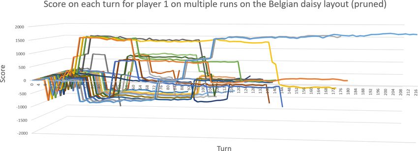
Chapter 1
Introduction
In the IEEE Conference on Computational Intelligence and Games, CIG
2012, Papadopoulos, Toumpas, Chrysopoulos et al. present a paper (from
hereon: source paper) on applying heuristics to an alpha-beta agent for the
game Abalone [1].
This thesis has two goals. The first goal is to verify and reproduce the results
of the source paper based on what was written about the implementation.
The second goal is to investigate the methods used and the decisions made
in the source paper.
Unfortunately, the source paper does not contain all the data to back up
their claims due to a reported page limit that the authors had to abide by.
As a result, many claims go unfounded, corners were cut in the method
descriptions and peculiar decisions were made that go unexplained.
This study aims to clarify the unfounded and unexplained parts of the source
paper and perform new measurements to see how they compare to the results
reported in the source paper. This should make it easier for future research
to build on the source paper as we will have filled the gaps that have been
left behind by the source paper.
To make measurements, we implement an Abalone alpha-beta game-playing
agent based on the source paper. In doing so, it becomes apparent which
aspects of the source paper are not backed up properly or explained poorly.
By running the game-playing agent with different settings, we can make the
necessary measurements to compare the performance of our implementation
with the claims from the source paper.
This thesis is structured as follows. In chapter 2 the required knowledge to
understand the rest of this material is explained. This is followed by the
methodology in chapter 3. Chapter 4 contains a critical review of the source
paper. Chapter 5 puts forward potential improvements to the evaluation
function metrics. In chapter 6 the obtained results are compared to the
results of the source paper. Next, the conclusions of this study are listed in
chapter 7. Finally, the discussion is held in chapter 8.

   The source code, release build, readme and raw results of the reimplementation of the
Abalone AI can be found at https://github.com/MichielVerloop/AbaloneAI.

                                           3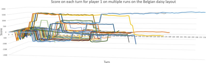
Chapter 2
Preliminaries
This chapter covers the required theory to understand the rest of this thesis.
It covers the goal and rules of Abalone, along with its technical characterist-
ics. In addition, the theory of minimax and alpha-beta is provided. Finally,
heuristics, extensions to the alpha-beta algorithm and other beneficial tech-
niques that are used are explained.

2.1     Abalone
Abalone is a 2-player strategy board game with perfect information and no
chance elements. Both players control 14 opposing black or white marbles
that are situated on a hexagonal board. The goal is to push six of the
opponent’s marbles off the edge of the board.

2.1.1    Rules
Starting positions
There are many starting positions that can be used, but only two of them are
relevant in this thesis: the default starting position and the Belgian Daisy
starting position. The default starting position has each player’s marbles
near the edge of the board, as shown in figure 2.1a. This starting position

 (a) The standard starting layout for       (b) The Belgian daisy starting layout.
 Abalone.

        Figure 2.1: The standard and Belgian daisy starting layout.

                                        4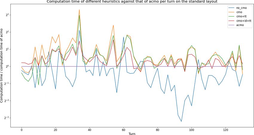
makes it easy to play very defensively, even allowing knowledgeable players
to force draws. This is an unfortunate oversight, which is accounted for in
the default starting position for tournaments: the Belgian Daisy starting
position.
In the Belgian Daisy starting position, half the marbles of each player are
isolated from their other half, as shown in figure 2.1b. This starting po-
sition creates more ‘interesting’ games: within a few turns, marbles can
be threatened and getting all of your marbles close to each other is more
difficult to achieve.

Moves
There are a few types of moves. The players take turn moving their marbles,
with black always making the first move.
First, the broadside move, which allows 2 or 3 marbles in a straight unbroken
line to move one space in a direction parallel to the axis of the line. This move
cannot push any marbles, so there cannot be any marbles at the destination.
Second, there is the inline move, which allows 2 or 3 marbles in a straight
unbroken line to move one space along the axis of the line. If there are
opponent marbles at the destination, then they can be pushed by the move,
provided the pushing marbles outnumber the opponent’s marbles and the
opponent’s marbles are not followed by another of your own marbles. The
opponent’s marbles can be pushed off the board by inline moves.
Moves can also consist of one marble, which can be moved one space in any
direction, thus treated as a combination of an inline and broadside move.
Because it can never outnumber any marbles, it can only move to empty
spaces.
Within this thesis, broadside moves are referred to as sidestep moves, inline
moves are referred to as sumito moves and moves consisting of a single
marble are also considered a sumito move. If a move pushes a marble off
the board, it is considered a capture move.

Game endings
The game is won by the first player that pushes six of their opponent’s
marbles off the board.
The game can also end in a draw, although the original rules that were
shipped with the physical Abalone game do not mention draws. There is
also no authority online that can be referred to for the rules, so instead,
we contacted the authors of the game, Michel Lalet and Laurent Levi, for a
clarification of the rules surrounding draws.
Together with the eight times Abalone world champion, Vincent Frochot,
they sent their response which can be found in the appendix A.1.
Essentially, a draw can occur after a sequence of eight moves. If both players

                                       5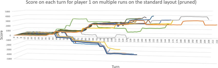
make and then undo their moves, they know that in response to each other’s
moves, they will undo their original moves, leading to the same game state
after four moves. If the players then repeat the same sequence of moves,
the game ends in a draw. If either player wishes to avoid a draw, they must
make at least one different move.

2.1.2    Technical characteristics
Abalone reportedly has a branching factor (number of possible moves per
game state) of 60 and an average game length of 87 moves [2, page 5], with
most games appearing to last anywhere between 50 and 200 moves [3].
For the implementation, there is a subtle but important difference between
game states, boards and moves. Game state refers to all information that is
known about a game of Abalone that is being played and includes the current
board. The board encompasses only the information that can be inferred
from looking at an Abalone board at a certain point in time. Notably, this
does not include information on whose turn it is.
A move consists of a set of coordinates and a direction, independent of
a board or game state. Notably, it does not consist of marbles which is
elaborated on in section 3.2. A move can be applied to a board or game
state if it is a legal move for that board or game state. Moves must be defined
in such a way such that the history heuristic can function, as explained on
page 10.

2.1.3    Known Abalone AI implementations
The most well-known and strongest Abalone AI implementation is Aba-Pro
from Aichholzer, Aurenhammer and Werner [4].
All other AIs that have been made for Abalone either have never been pub-
lished or are no longer publicly available. The AI created in the source paper
is among this group of ‘forgotten’ AIs. Despite publishing years after the re-
lease of Aba-Pro and referencing the Aba-Pro article on multiple occasions,
the source paper does not state that their AI played against Aba-Pro.

2.2     Minimax
For zero-sum games with perfect information, there are several different ways
to determine the best move in a given game state. The minimax algorithm
is one such approach to determine the best move. It works by exploring
all possible moves in a depth-bound depth-first search (DFS) manner. For
the final depth layer, all the game states (leaf nodes) are evaluated using
heuristics. The results propagate back to the moves at a depth of 1 where
the move that leads to the best game state is picked.

                                      6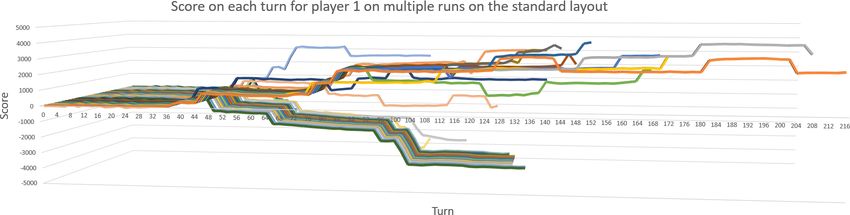
The propagation of moves is not completely straightforward as your oppon-
ent will be trying to maximize their score and work against you. Hence,
the algorithm assumes the worst-case scenario when predicting what the
opponent would do [5, ch. 10].

2.2.1   Evaluation
The previous paragraph briefly mentioned the evaluation of game states. We
seek to find a function which can approximate how advantageous a certain
game state is for the player. In essence, we want a method to quantify how
likely a player is to win in a certain game state. Such a function can then be
used by the minimax algorithm to determine what the ‘best move’ is when
looking ahead a certain depth.
For Abalone, the source paper differentiates between material and spatial
components in the evaluation function. The only material component is the
number of marbles captured by each player. The win condition is based
solely on this component, but that does not mean that the spatial com-
ponents can be ignored. Take the distance from center spatial component
for example. It describes how close the marbles are to the center of the
board. The closer marbles are to the center, the safer they are as it would
take many moves before such a marble could be captured. Hence, it feeds
into the material component: a low distance from the center leads to a low
likelihood of losing marbles soon thereafter.
The spatial components are not absolute indicators of how ‘good’ a game
state is, but they tend to approximate whether someone has an advantageous
board layout.

2.2.2   Alpha-beta
Alpha-beta is an adaptation to the minimax algorithm which filters out
moves that cannot lead to better moves than moves that have previously
been explored. It does so by saving the best values acquired at a given
sub-tree, then skipping branches that have a worse value.
To reason about the time save that alpha-beta pruning provides over mini-
max, we have to establish a few assumptions. We must assume a constant
branching factor b and a variable depth d.
The time save provided by alpha-beta pruning is dependent on the order
in which the nodes are discovered. In the worst-case scenario, the nodes
are discovered in order from worst to best meaning that no branches can
be pruned. The complexity that this yields, is the same time-complexity as
minimax: O(bd ). In the √
                        best-case scenario, most nodes are pruned, yielding
a time-complexity of O( bd ) [6, ch. 5].

                                      7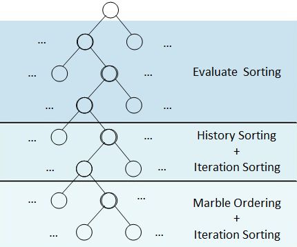
2.2.3   Iterative deepening
Iterative deepening is a search technique which searches the best move for
a given depth, then increases the depth limit and repeats this process until
either the final depth is reached or it exceeds the allocated amount of time.
Exploring the tree with iterative deepening will go more slowly than without
it as more work has to be performed, but due to the exponential nature of
minimax algorithms, it does not reduce the performance by an enormous
amount. The reduction in speed is bounded by a constant determined by
the branching factor. More specifically, the extra work has an upper bound
        1 −2
of 1 −        where b is the branching factor [7].
        b
Abalone has an average branching factor of 60 as noted in section 2.1.2.
When using the alpha-beta search, the effective branching factor lowers to
anywhere between 15 and 28. If additional pruning heuristics are applied,
the branching factor can further lower to anywhere between 5 and 8 [4].
This translates to a maximum of 56.3% ‘wasted’ work at a branching factor
of 5, and a maximum of 7.5% wasted work at a branching factor of 28.
The reason that iterative deepening is desirable despite slowing the calcula-
tions down is twofold. The option to cut off the search after a fixed duration
is highly desirable for practical applications. For example, this makes the
algorithm suitable for play against humans.
The second reason is that in practice, the results from shallower depths can
be used to speed up the exploration of subsequent depths and thereby mit-
igate how much longer iterative deepening DFS takes compared to DFS on
its own.

2.3     Transposition table
Evaluating a game state is a relatively expensive operation and only be-
comes more expensive as the evaluation function becomes more advanced.
A property of minimax algorithms is that the same game state is often vis-
ited repeatedly - after only two moves from each player, the same game state
can be reached using different moves. Hence, it becomes tempting to store
the outcome of the evaluation function on these game states in a technique
called memoization. With this technique, storage space and a bit of over-
head is traded for a significant reduction in the number of evaluation calls.
In addition to storing the rating of a game state, the result of evaluating
an entire branch can be stored. Storing branches yields even better time
saves as branches can be reused and need not be re-explored, making it as
effective as pruning branches.
To store this data efficiently, a hash table with a caching mechanism is
ideal as it provides a constant access time and bounded memory usage. The

                                      8
bounded memory is mandatory because the hash tables will easily exceed the
available memory if no measures are taken to restrict the memory usage. The
stored information can be accessed with a hash key obtained from Zobrist
Hashing.
2.4 Zobrist hashing
Zobrist hashing is a common hashing technique to create a hash for a game
state that can be applied to many board games. In constructing a Zobrist
hash, random values are assigned to specific combinations of material and
spatial components. Then, for all such components that exist in a certain
game state, the hashes are combined using bitwise XOR operation. The
result of this is the Zobrist hash of that game state [8].
Because XOR is self-inverse, the Zobrist hash of a game state resulting from
a move can be created by simply applying a bitwise XOR to the Zobrist
hash of the previous game state and the ‘Zobrist hash of the move’. The
Zobrist hash of the move is what you get if you only consider the values of
the combinations that change and XOR all of those.
All this gives Zobrist hashing two very desirable properties. First, it is very
cheap to generate a hash because it only costs a few XOR operations to do
so. Second, it allows the hash of a game state to be made before the game
state is visited, which can be useful in combination with hashing the game
results, evaluation sorting and history sorting.
In the context of Abalone, the combination of the color of a marble and its
position generate the random value. If later the same combination of marble
color and position occurs, the same value is returned as the first time.
2.5 Heuristics
For the scope of this thesis, we consider alpha-beta the ‘base algorithm’ on
top of which different heuristics are tested. These heuristics are presented
in this section.
2.5.1 Combined move ordering
Due to the nature of the alpha-beta algorithm, the order in which the moves
are supplied to the algorithm determines how quickly it terminates. The
practice of ordering the moves that alpha-beta agents take as an input is
called move ordering.
There is a balance to be struck between how computationally expensive the
move ordering heuristics are and how useful they are at a given depth. For
example, at the start of the tree, it is important to have the best ordering
possible because branches that are pruned early on prune more work than
9(a) Combined move ordering (b) Advanced combined move order-
ing
Figure 2.2: (Advanced) combined move ordering imagery taken from the
source paper. Both examples have evaluate sorting active on depths 1-3,
history sorting at depth 4-5 and marble ordering at depths 6-7. Advanced
combined move ordering additionally has iteration sorting active at depths
4-7.
branches at deeper depths. At the end of the tree, only one depth worth of
nodes can be pruned, meaning that it is more efficient to use less accurate,
yet cheaper sorting heuristics.
The source paper puts forward the technique of combined move ordering
which defines sections in the tree use distinct move ordering methods that
best suit that depth [1]. After introducing Iteration Sorting, they also put
forward the notion of advanced combined move ordering. Examples of the
different sections are shown in figure 2.2.
Evaluate sorting
Evaluate sorting is ordering the moves based on the evaluation of the game
state of the child nodes. Of all marble ordering techniques, this is by far the
most costly way to sort because it requires visiting and evaluating all child
nodes.
The accuracy of the evaluate sorting method scales with the accuracy of
the evaluation function, provided that game states that score high lead to
game states that are even better. Since we have no reason to believe this
requirement does not hold, we assume that it holds and treat the evaluation
function as the most accurate move ordering method.
History heuristic sorting
History heuristic sorting orders the moves based on the number of prunes
they caused. A move prunes branches when it leads to a branch with a good
enough alpha or beta score to cause other branches to not be evaluated.
10Filter
History Sorting Sort
Reorder front one-third and back one-sixth
Change relative position
Figure 2.3: Iteration sorting example taken from the source paper, altered
for increased clarity. First, a move ordering heuristic (here: history sorting)
is applied based on its metrics (here: kills/prunes). Afterwards, the moves
with known scores are filtered and sorted. This is used to reorder the front
one-third and back one-sixth of the moves, after which the relative position
of the remaining moves with known scores are sorted.
This heuristic is based on the assumption that a move that is good in one
board state is also good in similar board states [9].
This sorting method is cheaper than evaluate sorting as child nodes do not
have to be visited nor evaluated. Instead, the hash of a child node can be
created by combining the hash of the current game state and the hash of
the move that leads to the child node, as explained in section 2.4. This
hash is then used to look up the number of pruned branches it caused. The
moves are then sorted from high to low based on the number of branches
they pruned.
Marble ordering
This heuristic is specific to Abalone and was originally introduced in the
source paper [1]. This heuristic sorts moves by their types, sumito and
broadside moves, and on how many marbles are involved in the move.
The intuition behind the heuristic is that moves that involve more marbles
are more likely to impact the game in a significant manner as the turn is
utilized to a greater extent.
The heuristic is the cheapest of the move ordering heuristics as the sorting
process is very cheap. The moves can be sorted in linear time using a
counting sort or otherwise generated by type in linear time.
Iteration sorting
The authors of the source paper also put forward Iteration sorting [1], which
combines a cheaper version of the evaluation sort with the other sorting
11methods. This sorting method consists of two parts.
The first part consists of copying the list of legal moves and sorting both
lists using two separate sorting mechanisms. The first list is sorted based on
the hashed results from previous evaluation calls. The moves that haven’t
yet been hashed are ignored, thus reducing the size of the sorted list.
The second list is sorted using either history heuristic sorting or marble or-
dering.
The second part is to take the two sorted lists and combine them. Combin-
ing these lists is done by taking the best one-third and the worst one-sixth
moves from the first list. All moves in these parts of the list are removed
from the second list, after which the best one-third and the worst one-sixth
moves are added to the front and back of the second list, respectively.
An example of the combination of the history heuristic and iteration sorting
can be found in figure 2.3
The authors chose to move the worst one-sixth to the back because “in case
one of [the moves] turns out to be the only good one, being at the absolute
back will slow down [the] algorithm significantly”. No reason was provided
for why the first one-third specifically is moved to the front.
To work at all, iteration sorting has to make use of hashing. To make
it faster, it can be combined with iterative deepening. Doing so pays off
because interesting branches from lower depths get a more appropriate or-
dering, which leads to a lower branching factor, which improves the overall
speed.
All in all, iteration sorting allows you to reap the benefits from evaluation
sort, namely that it is the most accurate sorting method at our disposal,
without having to deal with its downside, which is that it is the most ex-
pensive of the sorting methods.
2.5.2 Quiescence search
Quiescence search is an extension to the alpha-beta search that, unlike most
heuristics, does not provide a speed-up to the search, but rather improves
the quality of the search. It does so by locally increasing the depth for leaf
nodes that have an ‘unstable’ score assigned to them, which causes the score
assigned to that node to be refined.
In the context of Abalone, a leaf node is considered to be quiet (stable) if no
marble captures occurred in the move leading up to it and it is considered
to be not quiet (unstable) when a marble capture did occur in the move
leading up to it.
The intuition behind quiescence search is that it alleviates the problems
caused by the horizon problem (also known as the horizon effect). This is
an issue that can occur due to the limited depth that the algorithm evalu-
ates. A game state can appear to be good in the leaf node, but might lead
to the loss of a marble in the next (few) moves.
122.5.3 Aspiration windows
Aspiration windows is a heuristic that provides the largest speed-up of all
the mentioned heuristics, at the cost of move quality. It works by pruning
all remaining branches when a move has been found that is considered ‘good
enough’.
The lower the threshold for ‘good enough’, the worse the move will be, but
the faster that move will be found. Conversely, if the standards for a good
enough move are very high, the move will be better but take longer to be
found. If the threshold is too high, no move will be found and a re-search
at a lower threshold has to be made.
Note that this differs from what the source paper considers to be aspiration
windows. The reason for this discrepancy is explained in section 4.4.
13Chapter 3
Methodology
In this chapter, we discuss our approach in critically analyzing and trying
to reproduce the results from the source paper.
3.1 Approach
To achieve the first goal of this thesis, verifying and reproducing the results
from the source paper, an implementation of the Abalone AI described in
the source paper had to be made. This implementation should allow for
different heuristics to be fairly compared against each other. An in-depth
view of how this is achieved is given in section 3.5.
The second goal of this thesis, to critically analyze the paper is aided by the
fact that the implementation was made without any help from the authors
of the source paper. This ensures that the contents of the paper are evalu-
ated without any external biases, making it easier to critically analyze the
contents of the paper.
3.2 Implementation considerations
There are some strict requirements for the Abalone implementation.
First of all, it must be possible to abort the computation of a move for
time-based Iterative Deepening to function.
In general, the representation of a move should be unambiguous. If there
are two move representations that describe the same move, the branching
factor will be unnecessarily increased, which leads to exponential perform-
ance losses.
For the History Heuristic, it is also important that a move is represented
independently from the board state, otherwise the History Heuristic cannot
function.
The move representation must also allow for Zobrist hashing. Zobrist hash-
ing requires that when the hash of a board state and the hash of a move are
combined using the XOR operation, the result should equal the hash of the
move applied to the board state.
For performance considerations, it is mandatory to make it possible to undo
a move. If no undo functionality is present, a copy of the entire game state
would have to be made for almost every move that is made during the search
which would be incredibly expensive.
14Next to the requirements, there are some decisions that should be made.
The first decision is which language and programming paradigm to use. In
this thesis, Java was chosen as the programming language because of the
author’s experience and affinity with that programming language.
Next, a trade-off has to be made between performance and code maintainab-
ility. The more primitive and efficient the board and legal move generation
are, the faster the AI will run as most of the computation time is spent gen-
erating all legal moves for board states. The downside is that implementing
other features may prove more difficult. In our implementation, the decision
was made to go for a less efficient but more easily modifiable program struc-
ture. This negatively impacts the absolute timing performance results, but
we hypothesize that the relative timing performance results will be similar
to that reported in the source paper.
3.3 Identifying criticisms
To identify weak points in the source paper, the question ‘why’ was asked for
every claim. If neither the context nor common (domain-specific) knowledge
could answer the question, it was added to the list of criticisms.
Criticisms were also identified during the implementation process as lacking
implementation details become especially apparent during that step.
3.4 Addressing the criticisms
After identifying the criticisms, the next step is to find out to which extent
they can be addressed. For some of the criticisms it makes more sense than
others to extensively address them. In this thesis, we only comprehensively
addressed the evaluation function as the source paper outlined that for future
research.
3.5 Comparing heuristics
There are several different ways in which to compare heuristics. One can
compare quality, speed, and the combination of these: performance.
To compare the quality of a heuristic, two identical agents repeatedly play
against each other, except one uses the heuristic that is to be tested, while
the other does not. There will not be a source of nondeterminism for this
measurement, so only 4 unique games can be created: two for each layout,
with both agents playing as the first player once. Because of this small
sample size, the results should be taken with a grain of salt.
To test speed, two agents, again with one differing heuristic will generate
15valid moves on a set of predetermined game states. Since both agents oper-
ate on identical game states, the comparison is not affected by the quality
of moves.
To test performance, the different agents repeatedly play against each other
on a time limit. As a result, during one execution the agent may return
the move computed at a depth of 3, whereas during another execution it
returns the move that was computed at a depth of 4. This leads to different
moves being used, and thereby branching of the games. This branching is
desirable as it allows more games to be evaluated than just the 4 in the case
of quality measurements.
Naturally, the win/loss ratio achieved by the quality and performance meas-
urements is used to determine the effectiveness of the heuristics used in these
measurements.
16Chapter 4
Critical review
This chapter delves into the decisions and claims made in the source paper
that are not self-evident or lack proper argumentation.
4.1 Training the evaluation function
The evaluation function as introduced by the source paper has 6 metrics
that determine the score of game states. These metrics should be assigned
weights to dictate their importance in the final score, else the evaluation
function would be a poor estimation of how valuable a game state is. The
source paper makes no mention of these weights or how they identify the
optimal values for these weights.
4.2 Formation break calculation
The source paper states the following on the formation break metric:
“Placing your marble among the opponent’s marbles has many
advantages. Not only your marble cannot be attacked, but also
the formation of your opponent’s marbles gets split in half. Thus,
they are less capable of attacking and become much more vulner-
able to being captured. This parameter is calculated as the num-
ber of marbles that have opponent marble in opposite sides.”
(Source paper, page 2)
In figure 4.1 there are three examples where the black marble is in formation
break, in line with the given definition. The above definition considers all
of these formation breaks equal. It does not consider multi-axis formation
breaks better or worse. In section 5.1, we investigate whether it is worth dif-
ferentiating between single- and multi-axis formation breaks and we discover
numerous other factors to consider.
4.3 Marble capturing danger
The source paper introduces single marble capturing danger as follows:
“When one of the player’s marbles touches the edge of the board,
while having neighboring opponent marbles, there is a possibility
17Figure 4.1: Three examples where the black marble in formation break.
From left to right, the formation break occurs on one, two and three axes.
of being captured. If there is only one, the reduction is minor. If
there are more than one opponent marbles the danger is immin-
ent and the reduction in the evaluation is high.”
(Source paper, page 2)
The source paper introduces double marble capturing danger as follows:
“The same goes when two of the player’s marbles touch the edge
of the board and have more than one opponent marbles on the
opposite side. This time the evaluation reduction is even higher
than before, because there are more than one marbles in danger.”
(Source paper, page 2)
From these definitions we can derive that the goal of the single and double
marble capturing danger metrics is to judge whether there is a high possib-
ility of one or multiple marbles being captured.
The problem with this metric is that it does not seem to reliably achieve
this goal. The metric creates a lot of false positives and false negatives
alike. One can devise many situations where the metric backfires and gives
the opposite score of what one would want. Two examples of this are given
in figure 4.2. Furthermore, the definition from the source paper does not
appear to differentiate between 2, 3 or 4 adjacent opponent marbles. In
figure 4.2a, the situation would be a lot worse for white if the white marble
in the top row were to be threatened by two additional marbles. The extra
marbles would mean that the white marble is trapped, allowing it to be
captured within two moves.
There is also no consideration for whether the marble that is in danger can
be pushed off in one move.
18(a) White would count three single (b) White would count zero marble
marble capturing dangers and one capturing dangers, while clearly be-
double marble capturing danger, des- ing at risk of losing a marble if it is
pite being in a position where they the black player’s turn.
can push off an opponent marble and
are not in danger if it is the white
player’s turn.
Figure 4.2: Two example situations where the marble capturing danger
metrics fail to evaluate the situation well.
The description of how the marble capturing danger metrics are implemen-
ted is also lacking. There is no information on how the two interact nor on
which numbers should be assigned to ‘minor’ and ‘high’ score reductions.
Finally, the single and double marble capturing danger metrics seem very
similar, which makes it an odd choice to create two metrics that are this
similar rather than to create one ‘danger’ metric.
To address these concerns, we put forward an alternative to these metrics
in section 5.2.
4.4 Non-linear aspiration windows
As was mentioned in the preliminaries, section 2.5.3, there is a difference
between the described aspiration windows and the aspiration windows that
were implemented by the source paper.
The approach taken by the source paper does not appear to align with what
is generally considered to be aspiration windows. While there is no clear,
concise and complete definition that we could find on aspiration windows,
the following seems to be a common pattern among various sources [9]–[12]:
The aspiration windows set a demand for how much better moves have to
be than the root node at a given depth. Iterative Deepening can be used
to better estimate the optimal value for this demand: the estimation of the
19best score at a given depth can be based on the best score at the previous
depth.
To reduce the branching factor, moves have to be significantly better than
the current best move as determined by alpha and beta. This reduces the
quality but saves a lot of time. To still provide quality guarantees, a move
is only used if it can guarantee a score equal to or better than the demand
that was set for the current maximum depth. If no such move is found, the
search is repeated with lower requirements until such a move is found or the
requirements cannot further be relaxed. This is called re-searching. If in
the end no move was found that can match the demand, the best move in
the last re-search is used.
All this vastly differs from what is described in the source paper. No men-
tion is made of either iterative deepening or re-searches in the context of
aspiration windows. The source paper only seems to implement or mention
the “moves have to be significantly better than the current best move as
determined by alpha and beta” aspect. They implement this by exploiting
“the use of the Alpha-Beta pruning, amplifying the window “cuts” with the
alpha-beta “cuts”. Thus, a and b can be derived as follows:”
estimation = evaluate(game)
a = max(a, estimation − windowsize)
b = min(b, estimation + windowsize)
The issue is that they never mention re-searches nor do they mention iter-
ative deepening in the context of aspiration windows, despite that being the
standard way to implement aspiration windows, to the best of the author’s
knowledge. Deviating from the standard is not necessarily bad. However,
given that non-linear aspiration windows are introduced as a novel concept,
the description and implementation of this should be clear and unambiguous.
Differences between the standard and new approach should be outlined, and
the differences in performance should be compared. Else, those that come
across the paper cannot make an informed decision between the standard
or altered approach to aspiration windows.
Another peculiar thing is that the speed-up claims differ each time perform-
ance comes up. In the section on non-linear aspiration windows, they state
that
“The performance increases up to tenfold compared to a simple
search in the same depth, sacrificing only a reasonable amount
of the quality of the result.” (Source paper, page 4)
However, in the experimental results section, they state
“Our player becomes almost twenty times faster, while losing
some of its quality due to the “guessing” procedure mentioned
20in III. [...] With this kind of “node economy”, you can search at
least two levels deeper in the same time, and thus increase the
quality again to a greater proportion.”
(Source paper, page 7)
This raises the question, which of these statements are correct?
Now let’s consider Aichholzer, Aurenhammer and Werner [4] and their im-
plementation of ‘linear aspiration windows’, which they refer to as ‘heuristic
alpha-beta’. They use a non-standard approach to aspiration windows, on
which the source paper seems to have based their approach. In table 1 of
that paper, the claim is made that it reduces the branching factor from 13
to 5 in the opening positions and from 13 to 8 in the ending positions. In
figure 5 of that paper, we can see that this corresponds to evaluating depth
9 with heuristic alpha-beta faster than depth 6 without.
The speed increase is far superior to that of the source paper’s approach
to aspiration windows, despite both implementations being trained to have
an agent with aspiration windows at a depth of d + 1 ‘marginally’ beat an
agent without aspiration windows at a depth of d.
Given that the source paper allegedly built on [4], it is the author’s opinion
that the source paper should have compared the results.
Finally, the source paper does not provide adequate information on how to
train the aspiration windows. Below is the only statement on the training
of aspiration windows:
“The most commonly used procedure for the determination of the
windows’ width is their gradual narrowing up to the point that
the Aspiration algorithm can marginally beat a one-level deeper
Min-Max Search. This way, the low degradation of the quality of
the player is guaranteed.” (Source paper, page 3)
Note that nothing was cited to back this up or provide further instructions
and that the word ‘marginally’ says very little in this context. It could
mean that the aspiration agent can beat the one-level deeper alpha-beta
agent only rarely, a little over 50% of the time, or almost always, where in
most matches it can barely manage to win.
4.5 Two-step hashing
In their section on transposition tables in the source paper, the authors
state the following about a flag to indicate whether a variable has been used
before:
“Every entry of the table can have a third variable, which will
act as a flag, indicating that the value has been used at least once
21before. This way, when a second-level hashing collision occurs,
the stored value is replaced with a new one, accordingly. The
purpose of this technique is to keep in store the more frequent
moves and replace the ones that have never been used.”
(Source paper, page 4)
Their replacement scheme is uncommon and not as practical as some of the
other choices [13]. If they clear their transposition table after each turn,
they are unable to benefit from previously explored turns. If instead they
keep their transposition table between turns, then getting to a game state
twice sets the flag and will prevent all future game states with the same
22-bit key from being stored, even if the original game state later becomes
infeasible or even impossible to reach.
Several of the replacement schemes outlined by Breuker, Uiterwijk and Herik
in [13] already solve the issue of keeping in store more frequent moves,
although they each come with their own disadvantages compared to the
replacement scheme of the source paper. For example, the replacement
scheme deep solves the above issue at the cost of storing a number instead of
a boolean. It is odd that the choice of replacement scheme goes unexplained
in the source paper.
4.6 Dealing with missing implementation details
In this chapter, we showed for several cases that there are lacking imple-
mentation details. In this section, we describe how the lack of information
is dealt with in the implementation.
The weights of the evaluation are untrained. The values assigned to it are
solely an estimate on the author’s part of what might be reasonable weights.
It would have been preferable to properly train these weights, but that has
been considered out of scope.
For marble capturing danger, we cannot derive an unambiguous implement-
ation, so we implement two versions. One which we believe is the closest to
what the authors describe, simply referred to as single- and double marble
capturing danger. One which we believe best achieves the goal of the de-
scribed heuristic, introduced in section 5.2 and referred to as immediate
marble capturing danger.
Non-linear aspiration windows are more difficult to get right. Because the
source paper does not go into how the non-linear aspiration windows or the
evaluation function were trained, and because the description of aspiration
windows lacks too many details, the decision was made to not implement
aspiration windows. Any implementation based on the description from the
source paper is unlikely to be similar to the implementation of the source
paper.
22For two-step hashing, we decided to go with the ‘new’ replacement scheme
for the sake of simplicity.
23Chapter 5
Evaluation Function
This chapter puts forward potential improvements to the metrics of the
evaluation function as per the criticisms presented in chapter 4.
The contributions of this chapter are purely theoretical. Whether the met-
rics provide the hypothesized effects and whether they actually improve
performance is left as future work.
5.1 Formation break calculation
As explained in section 4.2, the number of axes in which a formation break
occurs is not considered in the implementation of the source paper.
To judge whether it would be better to consider the number of axes when
computing formation break, we contacted Vincent Frochot, who won the
Abalone World Championship 8 times as of 2020. Frochot was kind enough
to reply and grant permission to attach his reply in the appendix, section
A.2.
Frochot states that (paraphrasing) a formation break on multiple axes can
be beneficial because it forces the opponent into a line of play if they want
to take control of the position that the marble in formation break occupies.
This grants the player that owns the marble in formation break a time
advantage, expressed in moves, which allows them to improve their position.
In his reply, Frochot also mentions another metric which he calls triangula-
tion. This metric is closely related to the formation break metric.
Triangulation occurs when three marbles form the corners of a triangle,
with one possibly empty field between each pair of marbles, as illustrated
in figure 5.1a. Such a position protects the marbles from 2 directions each
because it is not possible to fit 2 or more of the opponent’s marbles between
the marbles. With an extra marble, two triangulations can be formed to
protect the existing marbles from another direction, while the extra marble
would enjoy the protection of the existing marbles in these same directions.
When this idea is taken to the extreme, the result is a perfect triangulation,
as illustrated in figure 5.1b. In this situation, no white marbles can ever be
pushed.
Note that if a black marble were placed in between the marbles of a white tri-
angulation, the evaluation function will consider the triangulation of white a
good thing, while also considering the formation break of black to be good.
The explanation for this is simple: both a formation break and triangu-
24(a) An example of three marbles (b) One of the three perfect triangu-
forming a single triangulation. Note lations that are possible in Abalone.
that the marbles on the edge of the Regardless of where one can place
board can only be captured from one black marbles, white marbles are un-
direction. able to be pushed.
Figure 5.1: Examples of triangulation.
lation make it expensive (in terms of moves) to take over the location of
the marbles that form a formation break or triangulation. If there is no
desire from the opponent to take over the position, then the marbles met-
rics achieve nothing and may even be counterproductive by restricting the
movement of your own marbles.
We conclude that it is better to replace the question “Should a formation
break on multiple axes be considered better than a formation break on
one axis?” with “When is an opponent likely to want to take control of a
position?”. This leads to a notion of desired positions which could refine the
formation break and triangulation metrics.
5.2 Marble capturing danger
The issue with the marble capturing danger metric used by the source paper
is that it is prone to false positives and false negatives, as explained in section
4.3.
We have addressed this by putting forward our own version of the metric
that we call immediate marble capturing danger.
Immediate marble capturing danger is triggered if and only if a marble can
be pushed off within one move by the opponent.
By definition, there will be no false positives or false negatives for this metric.
This does not mean, however, that it is objectively better than single and
double marble capturing danger. These metrics are less accurate but apply
to far more situations. As a result, they may be indicative of a future
25Figure 5.2: Five example situations in which white marbles can be captured,
regardless of the actions white performs.
‘immediate marble capturing danger’ and steer the AI into a more aggressive
sequence of moves that allows it to capture the opponent’s marble.
Marble capturing danger can further be improved upon with another metric.
If a marble is immediately threatened, it can be checked whether that marble
can escape. If it cannot escape, you can assign most of the points that you
normally get for capturing the marble to the rating of the game state. This
then allows you to improve your position elsewhere on the board and only
decide to capture the marble if there is no better move. A few example
situations in which a marble cannot escape are given in figure 5.2.
5.3 Coherence
Our implementation of the coherence metric and the definition of the metric
differ as the definition was misinterpreted early on. The difference was not
caught until after generating the results, which is too expensive to redo.
Consider the definition of the coherence metric from the source paper:
“[Coherence] is calculated as the number of neighbors each marble
has, giving also an extra bonus in three marbles in-line forma-
tions.” (Source paper, page 2)
Compare this to the way the metric was implemented:
The coherence score of a marble is the number of allied marbles
surrounding it in a star pattern (figure 5.3a), where the outer
marbles only count if there is an allied marble between it and
the original marble.
The key difference between the two is that our implementation overly re-
wards long lines. The marble in the center of the star pattern is given the
26(a) The middle marble improves its (b) A typical formation that can be
coherence score for all of the other observed when our AI (white) plays
marbles on the board, for a total score against a stronger opponent. Because
of 12. of the coherence metric, it forms lines
that cannot influence the board in a
meaningful way.
Figure 5.3: Problems with our implementation of the coherence metric.
maximum score, while in reality it is often not a good use of marbles to cre-
ate such formations. After analyzing the games played by our AI, we found
that stronger opponents often amass a ‘powerful triangle’, next to which our
AI would form lines of marbles as illustrated in figure 5.3b. These lines are
vulnerable to being broken up by the powerful triangle without being able
to break up the powerful triangle itself.
To avoid overly rewarding long lines, we propose the following definition:
For each axis, for each marble, assign a score of 0 if it forms no
line, a score of 2 if it forms a line of length 2, and a score of 3
if it forms a line of length 3 or more. The coherence score of a
marble is the sum of the scores of all its axes.
No bonus has to be awarded for reaching a length of 3 as this is inherently
taken care of. Because each marble in the line contributes to the score, there
is a large reward for creating a line of 3 marbles. When a fourth marble is
added, however, it no longer improves the score of all the previous marbles,
making it less valuable. If the marble is instead placed adjacent to two of
the other marbles, the score increases.
5.4 Distance to middle
The distance to middle metric is as simple as it can get: sum up the Man-
hattan distance to the middle for each marble. The intuition being that the
middle gives versatility and safety. From the middle, marbles can quickly
27deploy to attack the opponent on any side without being in immediate risk
of being captured.
An alternative to distance to middle has been put forward by Aichholzer,
Aurenhammer and Werner [4] which they used as the sole metric for the
evaluation function of their Abalone game-playing agent, Aba-Pro. Instead
of computing the distance to the middle, this metric computes the distance
to the weighted average of the middle and the centers of mass of the black
and white marbles, respectively. The intuition is that “a strong player will
keep the balls in a compact shape and at a board-centered position.”
Vincent Frochot suggested pathfinding distance to middle as another po-
tential alternative. Such a metric would reward and punish based on the
freedom of movement of a marble in addition to staying safe. However, the
metric could be too expensive to be worth using.
Combining the two alternatives results in a weighted pathfinding distance
to middle metric which encourages a player’s marbles to stick together, be
close to the middle and close to the opponent’s marbles, while additionally
taking into account freedom of movement.
28Chapter 6
Results
We compare our performance results with the results of the source paper.
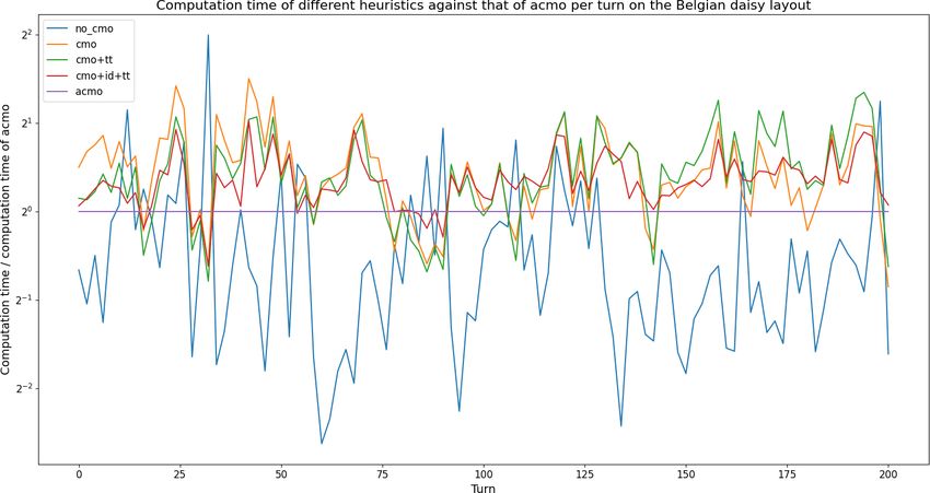
6.1 Internal consistency
Before we can produce results of any value, we must show that our method
to generate the data is not flawed. As explained in the methodology, in-
ternal consistency for timing is guarded by a consistent background load
for the computer1 and multiple executions of the same game. All runs that
measured performance, including the runs for other sections, were given an
arbitrarily chosen time limit of 15 seconds.
We observed that even after rerunning the same game 30 times, the min-
imum time spent computing a turn is around 4% slower with a background
load active. The minimum time spent computing the same turn is used
instead of the average as this better reflects the best possible performance
on the used hardware. Any results slower than the minimum time spent
computing are caused by small background processes that are infeasible to
eliminate. Even though we are mainly interested in the minimum time spent,
it is worth noting how much the runs improve when there is no background
load, as depicted in figure 6.1.
6.2 First-player bias
When putting two identical agents at odds against each other using iterative
deepening depth-first search to get nondeterministic executions, we observed
that the first player won 6 and 12 out 30 games on the Belgian daisy and
standard layout, respectively. Many of these games are barely different
from each other, to the point where (nearly) all moves are identical and the
games even end on the same turn. Such duplicate games are not interesting
in determining whether there is a bias, so we filter the runs to only leave
in a single of such duplicate runs. In this scenario, the first player wins 5
out of 15 games on the Belgian daisy layout and 11 out of 19 games on the
standard layout.
1
All results were generated on a Windows 10 system with an Intel Core i5-4590 cpu
with a clock speed of 3.3GHz running Java through AdoptOpenJDK JRE with Hotspot
11.0.9.11 (x64) which was given 4 GB of RAM.
29Figure 6.1: Internal consistency runs for Belgian daisy. In both graphs, the
computation times for 30 runs are plotted against the minimum computation
time for each turn. The difference between the graphs clearly show that a
background load has major influence on the computation times.
An odd pattern is that while games appear to be decided earlier, they are
also more diverse in the standard layout. We reason that the games are
decided earlier in the standard layout because both players want to take
the same positions, yet only one of them succeeds and gets the advantage.
In Belgian daisy, the AI finds multiple desired positions as there are two
clusters of marbles.
We suspect that the games are more diverse in the standard layout because
there are more turns where nothing game-deciding happens. The small
variations create disjoint games before the game it branches from is decided.
Additionally, for Belgian daisy we see (in appendix B.1) that the agents
always trade a marble at the start, which means that there are less marbles
to play with, leading to more similar games.
All in all, we conclude that there is a bias in the second player’s favor. To
mitigate this, we will be running all quality and performance measurements
twice as often so both players get to be the first and second player equally
often. For brevity’s sake, this will not be mentioned for each of the results.
6.3 Consider enemy position
A feature that was not considered in the source paper but which we imple-
mented is to toggle the computations of metrics for the opponent’s marbles.
We consider two agents: ‘consider self’, which only considers its own marbles
when rating the game states, and ‘consider enemy’ which considers both its
own marbles and that of the enemy when rating the game states. As ex-
pected, the quality is much worse for consider self than consider enemy: on
30Figure 6.2: The branching factor at depths 1-6 on both starting layouts, for
the AI that only considers its own marbles and for the AI that considers
both marbles. n refers to sample size; the number of turns where this depth
was reached.
both the Belgian daisy and the standard layout, consider enemy wins 4/4
times.
The performance, on the other hand, is far superior for consider self on the
Belgian daisy layout as it wins 20 out of 20 games. For the standard layout,
however, both agents are similar in strength: 9 out of 20 games are won by
consider self.
We reason that consider self is weaker on the standard layout due to both
AIs trying to get the same position (the middle), while only one of them can
attain this position. The AI that controls the middle generally wins.
The success of consider self on the Belgian daisy layout is explained by the
decrease in computation time. This decrease is a consequence of only having
to compute the metrics for half the marbles, and of a branching factor that
is, on average, lower than that of consider enemy, as can be seen in figure 6.2.
The lower average branching factor is presumably caused by the fact that if
there are less marbles to consider, the scores are more likely to overlap, and
therefore get pruned. In a way, this makes it similar to aspiration windows:
quality is sacrificed for speed to increase the overall performance.
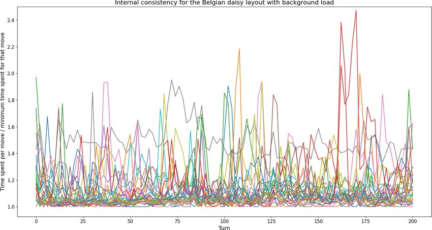
6.4 Speed comparisons
To verify the claims made by the source paper we compare the speed of
different heuristics as described in the methodology. In figure 6.3, the com-
putation times of the heuristics that each ran at a depth of 4 are plotted
against each other on a logarithmic scale for the standard layout. Because
the graph for the Belgian daisy loadout has a similar pattern to the standard
layout, it is included in the appendix instead of this section.
31You can also read