The Diablo 3 Economy: An Agent Based Approach
←
→
Page content transcription
If your browser does not render page correctly, please read the page content below
Noname manuscript No.
(will be inserted by the editor)

The Diablo 3 Economy: An Agent Based Approach

Makram El-Shagi · Gregor von Schweinitz

This version: May 6, 2014

Abstract Designers of MMOs such as Diablo 3 face economic problems much like policy makers in the real
world, e.g. inflation and distributional issues. Solving economic problems through regular updates (patches)
became as important to those games as traditional gameplay issues. In this paper we provide an agent
framework inspired by the economic features of Diablo 3 and analyze the effect of monetary policy in the
game. Our model reproduces a number of features known from the Diablo 3 economy such as a heterogeneous
price development, driven almost exclusively by goods of high quality, a highly unequal wealth distribution
and strongly decreasing economic mobility. The basic framework presented in this paper is meant as a
stepping stone to further research, where our evidence is used to deepen our understanding of the real-world
counterparts of such problems. The advantage of our model is that it combines simplicity that is inherent
to model economies with a similarly simple observable counterpart (namely the game environment where
real agents interact). By matching the dynamics of the game economy we can thus easily verify that our
behavioral assumptions are good approximations to reality.
Keywords Agent based models · economic mobility · heterogeneous price development

JEL-Classification: E31; D31; C63

Makram El-Shagi
California State University at Long Beach, Department of Economics, E-mail: makram.elshagi@csulb.edu
Makram El-Shagi · Gregor von Schweinitz
Halle Institute for Economic Research (IWH), Department of Macroeconomics, E-mail: gregorvon.schweinitz@iwh-halle.de
Gregor von Schweinitz
Martin-Luther-University Halle-Wittenberg, Chair of Macroeconomics
2                                                                                     Makram El-Shagi, Gregor von Schweinitz

1 Introduction

Over the past decade virtual gaming worlds – so called massive multiplayer online games (MMO) – gained
immense popularity. The more successful games such as World of Warcraft and Diablo 3 attracted more than
10 million players. However, what makes those games so interesting from the perspective of an economist, is
not (only) the commercial success, but that these game environments host complete virtual economies. These
economies face problems very similar to those encountered in the real world such as inflation, distributional
issues etc.1 The similarity between specific aspects of the real world and the virtual realities of MMOs
generated a new branch of literature, that essentially exploits MMOs as natural experiments (see e.g. Szell
and Thurner 2010). Several MMOs were sufficiently successful to generate quite vivid real-world markets
(mostly through ebay) for the in-game commodities and – more importantly – in-game money.2
    Economic aspects became so important in those games that updates (so called patches) often primarily
tackle economic issues, such as inflation. Essentially these patches can be interpreted as monetary policy.3
    The similarity of policy relevant economic issues in the real world and MMO economies inspired us to
develop a multi-agent model, reproducing economic features of one of the most successful current MMOs,
Diablo 3. In economic terms, we analyze an economy with heterogeneous commodities that are produced
and traded by heterogeneously endowed agents.
    Heterogeneous agent models have long been used to model price movements on a variety of markets
including commodity markets (see e.g. Kirman and Vriend 2001), financial markets (Palmer et al 1994;
de Long et al 1990) and monetary policy (Raberto et al 2008). What distinguishes our model from most
agent based models is first that we do not consider an economy fluctuating around a constant equilibrium but
a rapidly growing economy (with stochastic growth). Second, our model considers commodities where the
consumer’s choice is not about setting the quantity of the commodity he or she consumes, but consumers can
choose between different quality levels for similar products. Many existing commodities such as automobiles
share this feature. Rather than buying several cars, the typical consumer who wishes to spend more for
transportation would go for a better car. The same holds true (to a certain extent) for other commodities, such
as real estate and food, that represent a substantial part of spending. However, maximization of commodity
quality is rarely included in macroeconomic models.
    In this paper we focus on reproducing and analyzing some stylized facts of the Diablo 3 economy:
First, high quality commodities exhibit strongly increasing prices (that are often perceived as an expression
of a general inflation).4 . Second, goods of heterogeneous quality show a highly different price development,
something we call heterogeneous price development. Third, although the average quality of newly found items
remains constant, the average quality of traded items increases over time. Fourth, the price for each given
quality level of commodities follows a hump-shaped curve, where the price decline starts once better items
become widely available through trading. Fifth, we find that heterogeneous price development as observed
in Diablo 3 causes a highly unequal wealth distribution with very low economic mobility. And finally, we
find that loose monetary policy can cause a breakdown of the quantity relation.
    This paper is meant as a stepping stone to further research where our evidence is used to deepen our
understanding of the real world counterparts of economic problems we discuss. The advantage of our model
is that it combines the simplicity that is inherent to model economies with an observable but similarly
simple counterpart. By matching the dynamics of the game economy – where real agents interact – we can
thus easily verify that our behavioral assumptions are good approximations to reality. The remainder of the
paper is structured as follows. Section 2 motivates the relevance of our model. Section 3 explains our model
economy. Section 4 presents our results on price developments, as well as the wealth and income distribution.

    1The economic complexity of MMOs and their economic implications inspired Barnett and Archambault (2010) to analyze
the impact of MMOs on economic education.
  2 In the case of Diablo 3, our main example, there even existed a real money auction house within the game.
  3 Blizzard Entertainment (the publisher of Diablo 3) does not make actual game data available. However, ebay prices for gold

as reported in 1, designer interviews and the discussions in the Diablo 3 forums reveal the key features of price movements in
the game. A selection of quotes from game designers on the relevance of monetary policy, specifically targeting a recent patch,
is found in section 2.
  4 The problem of inflation in online gaming has plagued virtual economies from their very beginning. This even led to the term

mudflation, composed from inflation and MUD (multi user dungeon, i.e. the genre of the earliest multiplayer online roleplaying
games). For a literature review see e.g. Lehdonvirta (2005)
The Diablo 3 Economy: An Agent Based Approach 3
It also contains results from a monetary policy experiment and robustness checks for all important elements
of the model. Section 5 concludes.
2 Stylized Facts
2.1 Diablo 3
2.1.1 The game
Diablo 3 is an action roleplaying game (Action-RPG) that has been published by Blizzard Entertainment
in 2012. In Action-RPGs players control a character in a fictional setting, where they strive to fullfil game
objectives and defeat virtual enemies. During the game they improve the capabilities of their character both
by unlocking new abilities in the game and acquiring (”looting“) better equipment (”items“) that is left behind
(”dropped“) by defeated enemies. While most roleplaying games focus on telling a story (”campaign“) that
comes to an end once the player has played the entire game, Diablo 3 (like some other modern Action-RPG
titles) allows to repeat the campaign or parts thereof with a fully developed character at a higher difficulty
setting. At some point, when all abilities available for the character in the game are unlocked, the players
mostly attempt to improve their capabilities by aquiring better items to equip their character. Typically,
this part of the game, often referred to as end game, accounts for far more gaming time than the actual story
mode. Our simulation essentially aims to capture this end game.
In Diablo 3, a character can wield up to 15 different items (one headgear, one body armor, one pair of
boots, one set of shoulder protection, one set of gloves, one belt, one pair of trousers, two weapons, two
rings, and one necklace. All but four of those items can be further improved by using so called jewels. The
number of jewels per item is limited to one, except for the pair of trousers (with two slots) and the body
armor (with three). Items of all quality levels, gold – i.e. the in-game currency – and low level jewels are
dropped by enemies during the game. Better jewels, which are typically what matters in the end game, have
to be purchased at an in-game vendor at a cost that increases exponentially with jewel quality.
A special feature of Diablo 3 was the auction house. Although the game is played alone or in small groups
of at most four people, the auction house allowed all players on one continent to interact on a single market
to sell and buy items, greatly reducing transaction costs. Given the number of active players – 15 million
copies of the game have been sold, and in 2013 there were still 1 million active players a day – the auction
house was one of the most active markets in a virtual world.
The auction house gave players the opportunity to use (in-game and real world) money as a substitute for
playing time. which in the end game consists of tediously repeating similar tasks. Despite – or rather because
– it was heavily used, it was strongly criticized. A frequent criticism was, that it encouraged players to spend
too much time trading rather than playing. Improving the economics of the game became one of the primary
objectives of game development (rather than improving the game mechanics itself). Keeping casual gamers
motivated to actually play the game became increasingly difficult due to two reasons. First, the availability
of high quality items in the auction house made drops from enemies increasingly inattractive. Second, the
auction house increased transparency on the availability of high quality items, allowing inferences on the
income and wealth of few hardcore gamers.5 Moreover, the in-game currency was no longer primarily used
to trade with in-game vendors, which have fixed prices. Price stability (or rather the lack thereof) suddenly
became a problem in the virtual world as much as in reality.
Eventually the critique became so severe, that the auction house was closed in March 2014. However,
although Blizzard does not reveal data on the in-game economy, this two year experiment gave a lot of
opportunity to observe the development of an economy, where actual people interact, in fast motion.
2.1.2 Economics and economic policy in the game
As mentioned before, rising prices of items of high quality quickly became one of the key issues of the game.
The exchange rate between Diablo 3 gold and the Euro fell by 75% in merely three month between October
5 The negative effect of the auction house on the incentives of players to actually play the game is described in a newspaper
article “Why Diablo’s Auction House Went Straight to Hell”, Wired Magazine, 20. September 2013 (see http://www.wired.com/
2013/09/diablo-auction-house).4 Makram El-Shagi, Gregor von Schweinitz
2012 and January 2013. Figure 1 shows the price of gold pieces (gp) for European Diablo 3 servers on ebay
since October 2012. The ”exchange rate“ depreciates strongly over time, reflecting similarly high in-game
inflation.
Fig. 1 Price of gold pieces (gp) in Diablo 3 on Ebay
Note: The different markers indicate different stack sizes offered on ebay. We exclude smaller stack sizes due to large transaction
costs included in the prices (stack sizes of 5 mill. gp are traded at roughly 10ct. / mill. gp more than the displayed stacks). All
prices are obtained from one large scale trader on ebay.
While the Diablo 3 gold price might seem low, and does indeed reflect strong inflation, it has to be
considered that at the time when this data was collected, many items were sold for several 100 mill. gp in
the in-game auction house. Success or failure thus had significant economic implications at least for some
players.
This is one of the reasons why economic policy, in particular concerning inflation and income distribution,
quickly became a key issue in the regular updates of the game. The following quotes from senior game
designers of Diablo 3 have all been drawn from the Q&A concerning patch 1.0.7, see https://eu.battle.
net/d3/en/forum/topic/6609341108.
At this time a key issue in the game was the creation of ”gold sinks“, i.e. opportunities in the game to
spend gold at in-game vendors, thereby removing it permanently from the economy and thus reduce money
supply.
(1) Andrew Chambers (Senior Game Designer) on inflation problems:
We also need more end game item and gold sinks.The Diablo 3 Economy: An Agent Based Approach 5
(2) Andrew Chambers on monetary policy aspects of patch 1.0.7:
The Marquise gems are gold and item sinks (which is something we feel the economy can really benefit
from right now), and very attractive ones at that.
An important goal with the new Marquise gems is to act as a gold and Radiant Star gem sink. Cur-
rently, there’s nothing in the game that actually pulls those gems out of the economy, but to keep their
value up, that’s important.
(3) Wyatt Cheng (Senior Technical Game Designer) on price dispersion:
Anybody who has spent time looking at high-end items knows that the value of items at the best items
increases at an incredible rate. The difference between a 98th percentile and 99th percentile item can
increase the value by tenfold or more.
Besides the general problem of inflation, the game designer’s discussion reveals the increasing price spread
between the majority of items and a few high quality items, which are typically only marginally better.
That is, items display a different price development for different qualities, which we call heterogeneous price
development.
This is mostly due to the fact that items in the Diablo 3 economy are commodities with a supply that is
inelastic in the short run, and buyers decide on the quality of the commodity to purchase, rather than the
quantity. Since players can only use one item of a specific type, rather than having an array of good items
of the same type, it is more efficient to have a single excellent item of this type.
This is one of the key features of the Diablo 3 economy that our model replicates and that distinguishes
our approach from most macro models that use homogeneous goods, where increasing consumption of the
representative consumer reflects increasing quantities.
2.2 The real world: Why it matters
At a first glance it might seem, as if the afore mentioned focus on goods where consumers choose the quality
rather than the quantity to consume is a very restrictive assumption in the real world. However, a closer look
reveals that those goods are highly important. Individuals with higher income and wealth do not eat more,
they eat and drink better; they do not demand more transportation but choose a more convenient mode of
transportation such as a more luxurious car. And while they can afford bigger houses, the key choices are
about amenities and location.
For many of those products the supply is inelastic in the short run at least in the high quality segment;
e.g. the truly expensive wines are specific vintages from selected vinyards, and cannot be easily reproduced.
For other markets a much broader segment of the market shares this feature of price inelasticity of sup-
ply in the short run. Changing the supply of housing or cars might actually take years. As a consequence,
the observations on heterogeneous price development and price dispersion that hold for Diablo 3 also ap-
ply to these goods, as for example documented for real house prices in the U.S. between 1975 and 2005
(Van Nieuwerburgh and Weill 2010).
Additionally, these kind of goods account for a large share of spending. The expenses for rent or the
owners equivalent rent accounted for 31.6% of consumption expenditure (as defined in the CPI) in the US
in 2007. ”Motor vehicles“ (including purchase and maintenance, but excluding fuel, insurance etc.) account
for roughly 8% more. That is, at the very least almost 40% of spending decisions are actually concerning
commodities where the choice is about quality rather than quantity and where supply is inelastic in the short
run.
For commodities sharing those features where more disaggregated price data is easily available, we see
substantial differences in the price development over different quality segments. Figure 2 compares the US
CPI to two art prices indices describing the price development in the market for painting by the Dutch
Masters. The ”Top 10“ line, representing the top decile of the quality distribution, outperforms the CPI
by far, tripling the price relative to CPI commodities in merely 23 years. This is not all due to a generally
increased demand for art. While the ”Central 80“, i.e. the prices in the eight central deciles of the distribution
do outperform CPI on average, the difference is far less pronounced.6 Makram El-Shagi, Gregor von Schweinitz
900
Central 80
Top 10
US CPI
800
700
600
Price Index
500
400
300
200
100
0
1975 1980 1985 1990 1995 2000
Year
Fig. 2 US CPI and two art price indices covering paitings by Dutch Masters.
Note: data on the art price indices are drawn from http://www.artmarketresearch.com/graphs/sample_fr.html.
Commodities are not the only examples showing such a behavior. It also resembles two observations
from the economics of superstars. First, earnings are highly unequally distributed between few very talented
individuals and the rest of the population. Second, payments of superstars increases with the size of their
“benchmark” market. That is, the average level of CEO payment (in large firms) is linked to market capital-
ization (of large firms) (Gabaix and Landier 2008). In our model, increasing money supply will affect prices
of the best items over-proportionally, leading to a highly unequal wealth distribution among players.
3 The model
Despite the empirical importance of commodities with heterogeneous quality and inelastic supply, most
established macro models use the assumption of homogeneous goods. Our agent based model, inspired by
the Diablo game, fills that gap, establishing a simple agent based macro framework, that focuses on the type
of commodity described in this chapter.
3.1 Basic setup
Our model world consists of N heterogeneously endowed, myopic agents – labeled players – who aim to
maximize their utility using simple heuristics. For simplicity, we assume that utility is monotonically related
to the “power” ψ of a player that determines a players chances to produce more gold and find new items.
While our agents are identical in terms of preferences, they differ in their endowment with production factors
in each but the first period.
Production of power is using two production factors: items that can be found by the player and jewels
that have to be purchased from in-game vendors using gold (money) g that – as items – is found by the
player. Both jewels and items come in a range of qualities, jewel quality j is discrete, while item quality i
is continuous with good items being scarcer. Each player can only use one item and one jewel. That is, the
production of power depends on the quality of a players best item (and jewel) rather than the aggregate
quality of all items (jewels) he or she holds. The chances to find items and gold depend on the players power.The Diablo 3 Economy: An Agent Based Approach 7
Thus, the power of a player ψ can be considered as an intermediate good for the production of gold and
items.
Production – i.e. gaming – happens in turns where players act independent of each other. The only
interaction between players occurs in between the turns, when items are traded for gold in an auction house.
There is a proportional fee f for any transaction in the auction house that depends on the price of the traded
item.
This fee and the jewel cost are essentially used to withdraw gold (i.e., money) from the model world.6
Together with the gold production function these two are the main instruments of monetary policy.
3.2 Production and playing phase
Production function: In each turn t ∈ {1, . . . , T } each player n ∈ {1, . . . , N } produces power ψ using a
standard Cobb-Douglas type production function:
β
ψ(it,n , jt,n ) := ψt,n = iα
t,n jt,n , (1)
where it,n and jt,n are the item and jewel (quality) used for production by player n at time t. Every
player n has identical initial endowments i0,n = 0.5, j0,n = 1.7 Depending on the intermediate good ψt,n the
player is rewarded with both gold and the chance to draw d items, where
E(dt,n ) = ψt,n , (2)
i.e. on average player n gains a number of items dt,n equal to his power in round t. For this simulation
we induce uncertainty through the quality of items rather than the quantity. Thus, we keep the variance in
the number of draws conditional on ψ as low as possible, by assigning one item per full point of power and
one additional item with a probability corresponding to the fractional digits (a Bernoulli distribution), i.e.:
dt,n = bψt,n c + B(ψt,n − bψt,n c), (3)
where prob(B(x) = 1) = x and prob(B(x) = 0) = 1 − x for x ∈ [0, 1].
The quality of each item is drawn from a χ2 distribution with one degree of freedom. In subsection
4.3, we also present results for other distributions of item quality. They all share the characteristics that
item qualities are strictly positive and unbounded. Positivity is required for the Cobb-Douglas-production
function. The unboundedness ensures that it is always possible (although increasingly unlikely) to find a
better item.
With g denoting the quantity of gold held by a player, we assume that a scaling factor A determines the
earned amount of gold ∆g:
∆gt,n = Aψt,n . (4)
Heuristics for looting and selling: After production (but before the auction) each player decides which item
to keep, which items to sell to the in-game vendor at a price equal to their quality, and which items to put
on for sale in the auction house.
We assume that each player always keeps his best item. That is, whenever an item is found that is better
than the currently equipped item, the new item is used by the player himself and swapped for the original
item. Therefore, the player does not consider the possibility to improve himself by selling his best item and
using the return to purchase jewels.
The players form simple expectations about the chance to actually sell an item in the auction house.
Since items can be sold to the in-game vendor and players prefer to have a high budget for buying items in
the auction, they sell items below a certain quality threshold to the in-game vendor (assuming that these
items could not be traded in the auction house). This threshold is set to θ = q min(iAH AH
t−1 ), where it−1 is the
6 The necessity of “gold sinks” is highlighted in designer quote (1) in Section 2.
7 The initial item endowment is chosen to be smaller than the expected value of newly found items, ensuring that the initial
endowment is obsolete after very few rounds for all players. Therefore, adding heterogeneous starting endowment of agents does
not affect results.8 Makram El-Shagi, Gregor von Schweinitz
vector of item qualities that have been successfully sold in the auction house in t − 1, and 0 < q < 1 is a
discount factor. Items above that threshold are offered in the auction house. This heuristic item placement,
and especially the level of q does not affect the results (if it is not set too high), but limits computer runtime.
3.3 The auction and jewel buying
Each item put up for sale through the auction house enters with a minimum price that guarantees, that the
return after paying the transaction fee is at least as high as the quality of the item, i.e. the prices that would
be paid by the in-game vendor.
Each player aims to buy the item that maximizes his production in the next turn, taking into account
the jewels that can be bought (at a known price) after the item auction. That is, players are myopic since
they do not consider the possibility to save for a better item in the far future, but are rational as far as short
run optimization is concerned.
We use a simultaneous ascending auction (Milgrom 2000; Cramton 1998). That is, all items are sold at
the same time, the players know the current bid for all items, and bidding continues until no player is willing
to place another bid. The price paid for an item is just exceeding the second highest price that any player
would have been willing to pay.
Our reason for using a simultaneous ascending auction rather than a sequence of English auctions or
Vickrey auctions, is that the price a player is willing to pay for a specific item depends on the price of all
other items. This is mostly due to the fact that the marginal productivity of an item depends on the potential
jewel endowment and thus implicitly on the remaining budget. To compare items it is thus necessary to know
both their quality and their (current) price. The simultaneous generation of prices in our type of auction
accounts for this aspect.
Our auction is closely related to the dynamic auction for heterogeneous goods proposed by Ausubel
(2006). We impose two restrictions. First, the quantity of each heterogeneous good in the auction is one.
Second, agents will only purchase at most one item from the auction. That is, goods are strict substitutes
in the sense that an additional good (of a worse quality) provides no additional utility.
After the auction, players buy the best jewel that is available for their remaining budget. The price for
a jewel is denoted by P (j). We require the players to buy jewels sequentially. For convenience we define the
necessary payment for a jewel of quality j for player n already possessing jewel jt,n :
j
X
P̃ (j, jt,n ) = P (ι). (5)
ι=jt,n +1
Details on the computational implementation of the auction house and its translation into the framework
of Ausubel (2006) are given in the Appendix.
4 Results
4.1 General findings
To evaluate the general behavior of our model, we simulate it using the parameters given in Table 1.
The number of players N is chosen to guarantee enough “activity” in the game. That is, items over a
broad range of qualities are available at any time in the game. Frictions, such as the lack of availability of
adequate items, are only relevant to the best few players. The number of periods T covered by the simulation
is set high enough to make sure that we can shock the system at a point in time where initial conditions
(such as the initial endowment) no longer matter and we still have sufficient periods to observe the entire
impact of a shock to the system. We use a standard Cobb-Douglas production function with item elasticity
α and and jewel elasticity β. The technology of gold production is a scaling factor A. The auction house
threshold q is set to a level, where the probability that a player would buy an item excluded from the auction
house is close to zero. The auction house fee f is set according to Diablo 3.The Diablo 3 Economy: An Agent Based Approach 9
Parameter Specification
N 1000
T 1000
α 0.5
β 0.5
A 10
P (j) 2j
q 0.7
f 0.15
item draw function χ21
Table 1 Parameter specifications
Note: General parameters are the number of players N and the number of turns T ; production parameters are the elasticities
α and β and the technology of gold production A; auction relevant parameters are jewel prices P (j), the scaling parameter q
for the auction house quality threshold θ and auction fee f .
Experiments with other parameter values for the production function show, that our results are fairly
robust with respect to the production function, as long as the jewel pricing function fulfills two weak assump-
tions: Pricing remains restrictive for players who are already well equipped, but the price for low quality jewels
is not prohibitively high for poor players. These and other robustness checks are presented in Subsection 4.3.
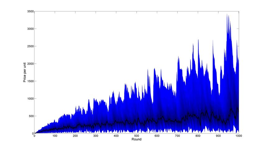
Prices: The results on price development are mixed. The median price per quality unit is increasing strongly
over time. The median of prices per quality unit and their density (obtained from a typical simulation) are
given in Figure 3.
However, increasing prices per quality unit are not necessarily a sign of inflation in the usual sense, as
they do not account for increasing quality. The increasing price per quality unit is mostly driven by an
increasing share of high quality items which yield a higher price per quality unit over the entire simulation.
Therefore, Figure 4 shows the median price per quality unit along with a Fisher price index, that accounts
for price changes of items of different qualities weighted by their expenditure share.8 While the median price
per quality unit is slowly increasing (0.64% per round), the Fisher price index decreases steadily after the
first few rounds at a rate of roughly 1.7%. Yet, the increasing cost for small improvements of a character’s
equipment when having to replace items by successively better items might contribute to perceived inflation
(see e.g. Jonung and Laidler 1988), as it is apparently prevailing in the actual Diablo 3 economy.
Moreover, a more disaggregated look into price movements reveals some substantial differences across
the different quality levels that might augment this perception. The observed deflation is clearly driven by
the bulk of low to medium quality items that rapidly loose value. But although there is no inflation on
average when accounting for quality differences of items, the prices of the best items currently available on
the market are usually strongly increasing.
Especially in the later game, when everybody is well equipped and only exceptionally rare items are
traded at all, the items available in the auction house are fairly homogeneous. From the 50th round on, the
contribution of the best decile of traded items to the total quality of traded items is usually between 10%
and 12%. That is, the best traded items are only marginally better than the average traded item. At the
same time the contribution of the price of those items to the total price of traded items usually is between
25% and 40%. The inflation rate for the best decile is on average 1% higher. A look at the data generated
in the early phase of the simulation suggests that this margin is increasing when looking at more narrow
definitions of the high quality segment. However, due to the decreasing number of items that is traded over
time, it is impossible to track those quantiles (in a meaningful way) in a simulation with a number of agents
that still is computationally feasible.
Figure 5 shows the price development by quality range. For each individual quality range, prices initially
– that is, when this quality level becomes first available in the auction house – increase. Once the quality
8 The Fisher price index (or Fisher’s ideal index) is the same index number that is used by the Federal reserve to compute
the PCE (personal consumption expenditure) price index, i.e. the Fed’s main price index. We use the usual auction setup to
calculate virtual prices in round k + 1 for items that were traded in round k (and vice versa). The index is normalized to 100
in period 1.10 Makram El-Shagi, Gregor von Schweinitz
Fig. 3 Empirical price level density over time
Note: Only items that are actually sold through the auction house are considered. The median price in each period is given by
the black line.
1000 400
Median price per unit (left axis)
Fisher price index (right axis)
Median price per unit
500 200 Fisher price index
0 0
0 100 200 300 400 500 600 700 800 900 1000
Round
Fig. 4 Median price per quality unit and harmonized price index over time
Note: Only items that are actually sold through the auction house are considered. The median price in each period is given by
the black line.
level becomes available to a broader range of players, prices start to decline until the item is traded no longer
(due to lacking demand).The Diablo 3 Economy: An Agent Based Approach 11
1400
Quality Range: 7 to 8
Quality Range: 9 to 10
Quality Range: 11 to 11.5
Quality Range: 12.5 to 13
1200 Quality Range: 13.5 to 14
Quality Range: 15 to 15.5
Quality Range: 15.5 to 16
1000
Price per quality unit
800
600
400
200
0
0 100 200 300 400 500 600 700 800 900 1000
Round
Fig. 5 Price development by quality range
The extremely high prices of top level items lead to the strong positive skew of the price distribution
that can also be seen in Figure 3. This fits anecdotal evidence, see designer quote (3) in Section 2.
It could be that price development is purely driven by supply and demand instead of the amount of money
in the system. Let us assume for a moment, that our model featured a continuum of heterogeneously endowed,
myopic players instead of a fixed number. Then, supply of every possible quality would be continuously
increasing (as overall production increases), while demand for every quality would be decreasing (as more
and more players are equipped with better items). Therefore, price development for any quality range should
be monotonically decreasing. If price development was solely driven by supply and demand, such decreasing
prices for every quality range should also be visible in our model with a limited number of players. The
increasing prices for scarce goods of comparably high quality in Figure 5 point to increasing prices for these
type of goods. That is, there is evidence for a monetary component in the price changes. Yet, the price spread
is of course strongly driven by demand side aspects, as the demand for items of comparably low quality is
rapidly falling as the market reaches saturation.
This heterogeneous price development has some substantial implications for the distribution of wealth and
social mobility in our Diablo 3 economy. First, the extreme spread between high end items and marginally
worse substitutes will lead to a strong overestimation of inequality when computing the wealth of play-
ers based on market prices (compared to inequality based on production, i.e., income). Secondly, strongly
increasing prices of top level items make it more difficult to bridge this gap for previously less successful
players. This can (and in our case does) give rise to increasing social immobility. Both of these issues are
discussed in detail in the following subsection.
Production and distribution: Total production of the intermediate good increases steadily.9 However, the
increase in production (and thus the number of found items) does not compensate the decreasing probability
to find an item needed to improve a player. Due to the exponentially increasing prices of jewels, they cannot
serve as a substitute for items, either. Thus, the growth rate of production decreases over time.
9 We consider the intermediate good ψ instead of final goods (items i and gold g) since this allows to reduce production
to a single indicator. For any utility function, all information about expected utility is contained in the production of the
intermediate good. Due to the random nature of item quality this does not hold for actual utility.12 Makram El-Shagi, Gregor von Schweinitz
4
10
3
10
Wealth Coefficient
2
10
1
10
90% over 10%
95% over 5%
0
99% over 1%
10
0 100 200 300 400 500 600 700 800 900 1000
Round
Fig. 6 Wealth of highest and lowest quantiles.
Note: A log scale is used to allow a representation of all three wealth coefficient series in one figure.
This is also reflected in the income distribution, where income is measured by productivity. While income
becomes more and more equally distributed (as item and jewel quality of players converge), small income
differences become more and more persistent, as players can only improve their position in the income
distribution by finding a better item.
Since the production of a player is monotonically related to his jewels and items that represent the major
part (around 80%) of his capital, the ranking of players in terms of production is almost identical to the
ranking of players in terms of capital endowment (the rank correlation coefficient is above 0.98 for all but the
first 50 periods).10 However, we find (nominal) wealth to be distributed quite unequally. The huge difference
between income (production) distribution and wealth distribution reflects one of our findings from the price
analysis: items that are only marginally better yield much higher prices in the upper part of the quality
distribution.
Figure 6 shows the total wealth of the upper 10% (5% / 1%) percentile over the total wealth of the lower
10% (5% / 1%) percentile. Starting from perfect equality, inequality quickly increases for about 15 rounds
and then continues to grow at a low pace.11
While the original seed of inequality in our simulation is the randomness of the quality of found items,
it soon becomes self enforcing. Players who are initially lucky find more items and more gold, allowing
them to buy better items in the auction house. This is augmented by two facts. First, over time less items
are found that can improve any player due to the decreasing growth rate of production. In the later part
of the game most items traded in the auction house are not newly found, but are passed on from the
previous users. Second, increasing prices for items of high quality make these items unaffordable for poor
players. Therefore, economic mobility in the society decreases. As seen in Figure 7, moving between deciles
of the wealth distribution becomes more unlikely over time, shown by the increasing concentration of players
10 Wealth is calculated by the sum of available money, value of the jewel and estimated value of the carried item. The value
of an item is estimated by REML-optimization of penalized splines (Ruppert et al 2003). Price per quality is regressed on a
constant, round and quality, using 3rd -degree polynomials, ten knots for the rounds and 15 knots for quality (knots distributed
equally over quantiles). Round and quality are interacted. This semi-parametric method is chosen due to the highly complex
function explaining the price, that can already be seen from Figure 5.
11 In the log form growth after period 15 seems very low, but there still is a clearly significant trend.The Diablo 3 Economy: An Agent Based Approach 13
90
10 10
80
9 9
70
8 8
7 60 7
Decile in period 100
Decile in period 900
6 50 6
5 40 5
4 4
30
3 3
20
2 2
10
1 1
0
1 2 3 4 5 6 7 8 9 10 1 2 3 4 5 6 7 8 9 10
Decile in period 200 Decile in period 1000
Bartholomew’s immobility index: 0.1633 Bartholomew’s immobility index: 0.04578
Fig. 7 Economic mobility.
Note: This figure illustrates economic mobility by showing the movement between deciles of the wealth distribution over a time
of 100 periods. The origin of players is given on the y axis, the density over destination deciles is indicated by the colorbar. For
the income distribution, the figure would be virtually identical.
on the diagonal, where they move neither up nor down the social ladder, and Bartholomew’s immobility
index12 that goes to zero. At any point in time, downward movements (left of the diagonal) are usually
small but comparably frequent. Except for minor adjustments through changing prices of equipped items,
those movements do not occur due to losses in wealth. Instead, players are overtaken by more lucky players.
Upward movements (right of the diagonal) usually happen through finding an exceptional item. Therefore,
they can be much larger but occur less frequent. Since these findings are based on the ranking of wealth
(rather than absolute values), they similarly hold for the income distribution.
4.2 Monetary policy shock
As a monetary policy instrument we analyze the introduction of new expensive jewel levels to an economy
that is mostly saturated with the current top level jewel. This serves to remove gold from the economy and
reduce prices. Adding new jewels – with this very purpose – has for example been done in patch 1.0.7 (see
designer quote (2) in Section 2).
For our simulation we introduce a top jewel level of 13 in the first rounds of the game. This level is
reached by the median player roughly in round 250. Once 80% of the players possess a level 13 jewel, we
remove the restriction on jewel levels.
Unsurprisingly, the development in this policy scenario is almost identical to the baseline scenario in the
first rounds of the game, until the first players are actually restricted by the newly introduced quality cap for
jewels. From this point on, gold is accumulated much faster due to the missing “gold sink”, reaching a level
almost twice as high as in the benchmark scenario directly before the policy shock. Yet, despite this massive
increase in money supply, only partly transmits to item prices. The price level per quality unit is merely
20% above the level in the benchmark scenario. The Fisher index is only marginally above the benchmark
level. Apparently, a huge part of gold is hoarded rather than being spent, since players who are not able to
12 For an overview over social mobility measures including this one see Dardanoni (1993).14 Makram El-Shagi, Gregor von Schweinitz
2
Price per quality unit
Gold
CPI
1.8
1.6
Average policy / average without policy
1.4
1.2
1
0.8
0.6
0.4
0.2
0
T−600 T−500 T−400 T−300 T−200 T−100 T T+100 T+200
Round relative to policy shock S
Fig. 8 Relation of prices and gold between baseline and policy setting
Note: The results reported are calculated as the average of 100 simulations of the respective models.
purchase an item to improve their character have no alternative way to spend their money. Essentially, this
leads to a collapse of the quantity relationship, or – more precisely – the relation between prices and money
due to a strong reduction in velocity.
Directly after the shock, i.e. the introduction of new jewels, both the amount of gold and the two price
indices drop below the levels of the benchmark model more or less reestablishing the original relationship of
prices and money. The prices then approach benchmark levels slowly until the end of the game simulation,see
Figure 8.
Partly, this is linked to the distributional issues discussed above. The additional money is predominantly
earned by the rich who hit the jewel threshold much earlier, i.e. they have both higher income and more time
to save. Since the rich to not compete with the poor for the low quality items, the increasing money supply
does not translate to higher prices for those items. Since the purchasing options for the rich are limited,
money starts being hoarded. This highlights the importance of micro level analyses of the transmission
mechanism. Depending on how and where money enters the economy, the implications of increasing money
supply for price changes might differ strongly.
Although in our model inflation is a purely monetary phenomenon, the quantity relation does not hold in
the model with a jewel quality cap of 13. A substantial part of money is hoarded rather than spent because
neither a better jewel nor an appropriate item are available. That is why the ratio of gold between models
drastically exceeds the ratio of prices between models prior to the policy shock.
4.3 Robustness checks
We perform several robustness checks with different parameter combinations, item production functions and
jewel costs. In general, we find a very similar development of prices per quality unit as shown in figure 5 for
the baseline scenario. Our main results hold true: the heterogeneity of items found in the first periods leads
to an unequal distribution of production and income. While equality of production increases in the course
of the game, the differences become more and more persistent.The Diablo 3 Economy: An Agent Based Approach 15
500
Quality Range: 7 to 8
Quality Range: 9 to 10
Quality Range: 11 to 11.5
450
Quality Range: 12.5 to 13
Quality Range: 13.5 to 14
Quality Range: 15 to 15.5
400 Quality Range: 15.5 to 16
350
Price per quality unit
300
250
200
150
100
50
0
0 100 200 300 400 500 600 700 800 900 1000
Round
Fig. 9 Price development by quality range for quadratic function P (j).
Changing parameters: In a first set of robustness checks, we vary the number of players and turns, N and
T , the parameters of the Cobb-Douglas function, α and β, and the auction house fee f .
Changing the number of players or the number of rounds does not affect the results beyond the impact of
the random draw function. In a setup with a low number of players, prices per quality unit or more volatile,
and are strongly affected, if an exceptional item is found by chance in one of the first rounds.
Modifying the production parameters (keeping the sum equal to 1) effectively shifts the focus of players
between the purchase of items and jewels. That is, for higher α (and lower β), the contribution of jewels to
production decreases, and they become less attractive. Therefore, players are willing to pay slightly more for
good items. Correspondingly, the price development for every quality range becomes steeper, peaks earlier
and drops to unity faster. However, the development of prices is very close to the baseline scenario.
Increasing the auction fee f implies a tighter monetary policy, withdrawing a higher share of money in
every transaction and leading to lower item prices. As higher fees imply a smaller stock of money, better
jewels can only be bought a little bit later than in the benchmark scenario. However, the difference is so small
that total production is nearly unaffected. Therefore, the point in time when demand for certain items has
fallen to zero remains unaffected as well. Overall, prices are slightly lower for higher auction fees, reaching
their maximum level earlier and decreasing less fast afterwards.
Changing jewel costs: In a second set of robustness checks, we test if exponentially increasing prices for jewel
improvements are necessary to achieve our results. High prices for better jewels and scarceness of high-quality
items imply few investment opportunities and therefore a certain degree of money hoarding. If jewel costs
do not increase as fast as in the baseline scenario, there are more investment opportunities, reducing the
money stock and therefore also item prices. We test this theoretical result with two alternative specifications
of P (j): a quadratic function (P (j) = 10j 2 ) and a linear function (P (j) = 100j − 90). All other parameters
are kept at the baseline scenario levels. The factors (and the constant in the linear case) are introduced in
order to impose certain costs for higher-level jewels while keeping low-level jewels at moderate prices.
The results of these two experiments can be seen in figures 9 and 10. In both cases, the availability
of better jewels at lower prices implies increased production. Therefore, for the broad mass of players, all
item classes are faster available compared with the baseline scenario. Similarly, they become unattractive at
earlier points in time. As expected, prices per quality unit are also significantly lower than in the baseline16 Makram El-Shagi, Gregor von Schweinitz
300
Quality Range: 7 to 8
Quality Range: 9 to 10
Quality Range: 11 to 11.5
Quality Range: 12.5 to 13
Quality Range: 13.5 to 14
250 Quality Range: 15 to 15.5
Quality Range: 15.5 to 16
200
Price per quality unit
150
100
50
0
0 100 200 300 400 500 600 700 800 900 1000
Round
Fig. 10 Price development by quality range for linear function P (j).
scenario. Moreover, they decrease faster after their peak if jewel prices increases are less steep. However, the
main story of the development of prices per quality remains unaffected.
Changing item draw function: In a last set of robustness checks, we test the dependence of our results on
the type of item draw function. As the finding of a high-quality item in an early round translates into higher
gold and item production for every player, the tail size of the probability function describing item quality
might severely affect our results. To test that, we employ three additional distributions: An exponential
distribution, a lognormal distribution and a generalized pareto distribution. The baselines distribution, a
χ2 -distribution with one degree of freedom, has a heavier tail than the exponential distribution, but less
heavy than the two other ones (with the generalized pareto distribution having the heaviest tail). To be able
to compare the results with the baseline results, we calibrate the distributions to have a mean of 1 and (for
the lognormal and the generalized pareto distribution) a variance of 2.
The price development per quality unit is given in figure 11 for the exponential, 12 for the lognormal
and 13 for the generalized pareto item quality function. Heavier distribution tails translate into higher
probabilities for items of high quality. Therefore, it is sensible to use different quality ranges for every
distribution. The threshold for items in the auction house gives a good impressions of the strong influence of
quality distribution on the endowment of players. It is 13.95 in the baseline scenario in the final round, it is
8.1 for the exponential distribution, 31.7 for the lognormal and 30.8 for the generalized pareto distribution.
The availability of high-quality items also affects their prices relative to jewel prices (which are kept fixed).
Fatter distribution tails lead to lower prices per quality unit compared to the baseline scenario, although the
overall amount of money in the economy increases strongly. However, as in all other robustness checks, the
general development of prices per quality unit remain unaffected.
5 Conclusions and future research
Designers of MMOs such as Diablo 3 face economic problems much like policy makers in the real world.
However, opposed to the real world, economic aspects of the game as well as different monetary policies areThe Diablo 3 Economy: An Agent Based Approach 17
1800
Quality Range: 1 to 2
Quality Range: 3 to 4
Quality Range: 5 to 6
1600 Quality Range: 6.5 to 7
Quality Range: 7.5 to 8
Quality Range: 8.5 to 9
Quality Range: 9 to 9.5
1400
1200
Price per quality unit
1000
800
600
400
200
0
0 100 200 300 400 500 600 700 800 900 1000
Round
Fig. 11 Price development by quality range for exponential item production function with mean 1.
900
Quality Range: 5 to 8
Quality Range: 11 to 14
Quality Range: 17 to 20
800 Quality Range: 22 to 24
Quality Range: 26 to 28
Quality Range: 28 to 30
Quality Range: 30 to 32
700
600
Price per quality unit
500
400
300
200
100
0
0 100 200 300 400 500 600 700 800 900 1000
Round
Fig. 12 Price development by quality range for lognormal item production function with mean 1 and variance 2.18 Makram El-Shagi, Gregor von Schweinitz
700
Quality Range: 5 to 8
Quality Range: 11 to 14
Quality Range: 17 to 20
Quality Range: 22 to 24
600 Quality Range: 26 to 28
Quality Range: 28 to 30
Quality Range: 30 to 32
500
Price per quality unit
400
300
200
100
0
0 100 200 300 400 500 600 700 800 900 1000
Round
Fig. 13 Price development by quality range for generalized pareto item production function with mean 1 and variance 2.
comparably easy to model. Therefore, such a controlled game environment offers a fascinating opportunity
to study the effect of policies on monetary transmission, income and wealth distribution, etc.
Using an agent simulation framework, we find a heterogeneous price development for different goods,
where particularly strong price increases can be observed for goods of outstanding quality, while those of
average quality feature deflationary tendencies. The strong price dispersion causes strong differences in the
distribution of wealth. Although almost all “wealth” is productive in our setting, we find very small differ-
ences in income that decrease further over time, while wealth is distributed highly unequal with inequality
increasing over time as the price spread becomes larger. Social mobility starts out high, but diminishes very
quickly over time. All those findings mirror the corresponding anecdotal evidence.
When considering a world with artificial restrictions in the monetary policy section we can show some
more interesting features of our model world. Although there is no motive for holding money (in the sense
that it does not enter the objective function that players maximize when buying) and since there is not
even a motive for saving in our model, there can be situations when money is hoarded, that is, monetary
transmission is hampered and the quantity theory does not hold any longer.
In the current setup the players feature simple heuristics instead of forward looking behavior. Therefore,
in a next step the behavior shall be augmented by the formation of expectations that are considered when
making a decision to trade. The strong price fluctuations found in our model suggest that a certain level
of rigidities that would possibly result from the inclusion of expectations might be welfare enhancing when
considering risk averse agents. However, rejecting trades that are substantially worse than what has been
expected, causes rigidities that can in turn cause price development that reinforce themselves, essentially
creating bubbles in real assets. This gives rise to the question whether there is a socially and individually
optimal level of price rigidities. An augmented framework would thereby help to bridge the gap between
agent models on commodity trade and financial market agent models where expectations traditionally play
a stronger role.
An extension of our model, to account for population dynamics, would allow the analysis of economic
mobility with inter-generational aspects. The dynamics introduced by new players would stabilize prices for
items of lower quality (i.e. basic goods), while the exit of old players could reduce the price dynamics for
top-level items. While overall economic mobility might increase, it is unclear whether new players have a
realistic chance to catch up to the old “aristocracy” of the game.The Diablo 3 Economy: An Agent Based Approach 19
References
Ausubel LM (2006) An Efficient Dynamic Auction for Heterogeneous Commodities. American Economic Review 96(3):602–629
Barnett JH, Archambault L (2010) How Massive Multiplayer Online Games Incorporate Principles of Economics. TechTrends
54(6):29
Cramton P (1998) Ascending Auctions. European Economic Review 42(3-5):745–756
Dardanoni V (1993) Measuring Social Mobility. Journal of Economic Theory 61(2):372–394
Gabaix X, Landier A (2008) Why Has CEO Pay Increased So Much? Quarterly Journal of Economics 123(1):49–100
Jonung L, Laidler D (1988) Are Perceptions of Inflation Rational? Some Evidence for Sweden. American Economic Review pp
1080–1087
Kirman AP, Vriend NJ (2001) Evolving Market Structure: An ACE Model of Price Dispersion and Loyalty. Journal of Economic
Dynamics and Control 25(3):459–502
Lehdonvirta V (2005) Virtual Economics: Applying Economics to the Study of Game Worlds. In: Proceedings of the 2005
Conference on Future Play
de Long JB, Shleifer A, Summers LH, Waldmann RJ (1990) Positive Feedback Investment Strategies and Destabilizing Rational
Speculation. Journal of Finance 45(2):379–395
Milgrom P (2000) Putting Auction Theory to Work: The Simulteneous Ascending Auction. Journal of Political Economy
108(2):245–272
Palmer R, Arthur WB, Holland JH, LeBaron B, Tayler P (1994) Artificial Economic Life: a Simple Model of a Stockmarket.
Physica D: Nonlinear Phenomena 75(1):264–274
Raberto M, Teglio A, Cincotti S (2008) Integrating Real and Financial Markets in an Agent-Based Economic Model: an
Application to Monetary Policy Design. Computational Economics 32(1):147–162
Ruppert D, Wand MP, Carroll RJ (2003) Semiparametric Regression, vol 12. Cambridge Univ Pr
Szell M, Thurner S (2010) Measuring Social Dynamics in a Massive Multiplayer Online Game. Social Networks 32(4):313–329
Van Nieuwerburgh S, Weill PO (2010) Why Has House Price Dispersion Gone Up? Review of Economic Studies 77(4):1567–1606
Appendix: The auction
Implementation: Although our model players are virtual agents themselves, they make use of bidding agents
for computational reasons outlined below.
The bidding takes place in rounds, giving the players the chance to sequentially place their bids. In
detail, a bidding round looks as follows. The sequence of players in a round only matters if players have
identical willingness to pay and produces an outcome equivalent to truly simultaneous auctions otherwise.
Since gold endowment is continuous, the probability of two players having precisely the same willingness to
pay is zero.13
At the start of each bidding round τ of the auction, we check whether there is any player who cannot
afford any item increasing his power, or for whom buying jewels only is the optimum choice given current
prices. Since bids do not decline during an auction, any player meeting one of those criteria at any time in
the auction, also meets those criteria for the remainder of the auction. Therefore, all those players leave the
current auction permanently.
Because each player can only use one item, players who are currently highest bidders are not considered
in the current round of bidding.
A player n who is willing to bid first identifies the item that yields the highest power level considering
the maximum jewel level that he or she can purchase from the remaining budget. Labeling the current bid
for item m in bidding round τ with bτ,m , and j ∗ (gt,n − bτ,m ) being the maximum jewel level available for his
remaining gt,n − bτ,m gold, the objective of the player n thus is:
ψ(i∗t,τ,n , jt,τ,n
∗
) = max ψ(im , j ∗ (gt,n − bτ,m )). (6)
m
The player can then compute a maximum bid b̄t,τ,n that does not change his original considerations, i.e.
the bid for i∗ where he or she can still afford j ∗ :
∗
b̄t,τ,n = gt,n − P̃ (jt,τ,n , jt,n ). (7)
13 In real world applications (such as the sale of licenses to use bands of radio spectrum), collusion, risk aversion, and the
deterrence of bidders who expect to be outbid cause different outcomes between sealed bids and sequential bids where the
bids are immediately revealed (Cramton 1998). Since none of these problems apply in our (simulated) environment, we can
immediately reveal bids for computational simplicity.You can also read