Supports the Omnigenic Theory - bioRxiv
←
→
Page content transcription
If your browser does not render page correctly, please read the page content below
bioRxiv preprint first posted online Jan. 17, 2019; doi: http://dx.doi.org/10.1101/523365. The copyright holder for this preprint
 (which was not peer-reviewed) is the author/funder, who has granted bioRxiv a license to display the preprint in perpetuity.
                                  It is made available under a CC-BY 4.0 International license.

   Gene Expression Predictions and
   Networks    in  Natural   Populations
   Supports the Omnigenic Theory
   Aurélien Chateigner1*; Marie-Claude Lesage-Descauses1; Odile Rogier1; Véronique Jorge1; Jean-Charles
   Leplé2; Véronique Brunaud3,4 ; Christine Paysant-Le Roux3,4 ; Ludivine Soubigou-Taconnat3,4 ; Marie-
   Laure Martin-Magniette3,4,5 ; Leopoldo Sanchez1*; Vincent Segura1*
   1
    BioForA, INRA, ONF, Orléans, France
   2
    BIOGECO, INRA, Univ. Bordeaux, Cestas, France
   3
    Institute of Plant Sciences Paris-Saclay (IPS2), CNRS, INRA, Université Paris-Sud, Université d'Evry,
   Université Paris-Saclay, Bâtiment 630, Plateau de Moulon, Gif sur Yvette, France
   4
    Institute of Plant Sciences Paris-Saclay (IPS2), CNRS, INRA Université Paris-Diderot, Sorbonne Paris-
   Cité, Bâtiment 630, Plateau de Moulon, Gif sur Yvette, France
   5
    MIA-Paris, AgroParisTech, INRA, Paris, France
   * Equal contribution

   Abstract
   The recently proposed omnigenic model makes use of network theory to distinguish central (or core) from
   peripheral genes underlying phenotypes. Core genes are typically few, they marginally contribute highly
   but altogether explain only a small part of trait heritability, while peripheral genes, each of small influence,
   are so numerous that they finally lead risk. In order to test this model, we collected and sequenced RNA
   from 459 European black poplars. We built the coexpression networks to define core and peripheral
   genes as the most and least connected ones. We computed the role of each of these gene sets in the
   prediction of phenotypes, with a linear additive model and an interactive neural network model. These
   analyses showed that core genes act directly and contribute additively to phenotypes, consistent with a
   downstream position in a biological cascade. Oppositely, peripheral genes interact to influence
   phenotypes, consistent with an upstream position. Overall, our work is the first empirical proof that
   omnigenic holds in trees, providing one step further towards the universalization of this model.

                                                                                                                                    1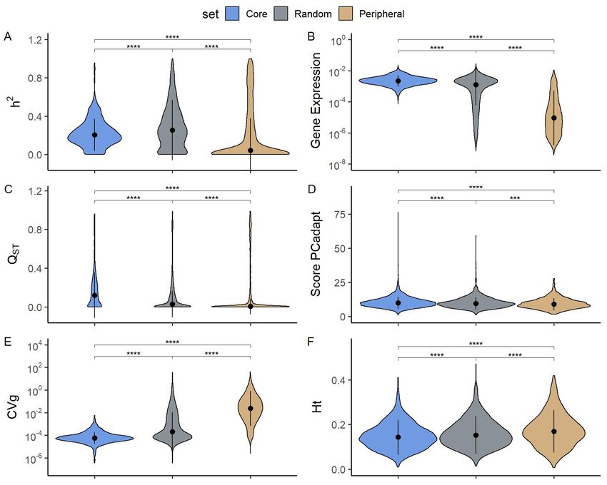
bioRxiv preprint first posted online Jan. 17, 2019; doi: http://dx.doi.org/10.1101/523365. The copyright holder for this preprint
 (which was not peer-reviewed) is the author/funder, who has granted bioRxiv a license to display the preprint in perpetuity.
                                  It is made available under a CC-BY 4.0 International license.

   Introduction
   In a recent study, Boyle, Li, and Pritchard1 proposed the omnigenic theory, as an extension of
   the classic polygenic view for the genetic architecture of complex traits. They provide a clear but
   human-centered definition of their new paradigm explaining that numerous genes that are
   peripheral in a regulatory network are sufficiently connected to genes directly involved in a
   disease to modulate their effect and recover most of the missing heritability of the disease risk2.
   They conclude by inviting the community to test this hypothesis with empirical data. For that
   matter, the most obvious approach would be to infer gene networks and study the role of
   modules of different topologies in the definition of phenotypes. In the present study, we are not
   only going to test this theory with real empirical data, demonstrating the importance of centrality
   in the prediction of phenotypes but also extending the range of application to another kingdom:
   plants.
   Two studies published just before Boyle’s were already framing the subject within the plant
   kingdom. Josephs et al.3 studied the link between previously published concepts related to gene
   expression4, gene connectivity5, divergence6 and traces of natural selection4,7. They showed
   that both connectivity and proximity on the genome are important factors, while not being able to
   disentangle which of them is directly responsible for patterns of selection between genes. A
   week after, Mahler et al.8 recalled the importance of studying the general features of biological
   networks in natural populations. With a genome-wide association study (GWAS) study on
   expression data from RNA sequencing (RNAseq), they suggested that purifying selection is the
   main mechanism maintaining the connectivity of core genes in a network and that this
   connectivity is inversely related to eQTLs effect size. These studies start to outline the first
   elements of the omnigenic theory, stating that core genes, which are highly connected, are each
   of high importance, and thus highly constrained by selection. On the opposite side of the
   network, there are peripheral, less connected genes, never far from a core hub, and each of low
   importance. These peripheral genes are less constrained genes and consequently, they harbor
   larger amounts of variation at population levels, concording with the omnigenic theory.
   Classic studies of molecular evolution in biological pathways showed that selection pressure is
   correlated to the gene position within the pathway, either positively9–14 or negatively14–17,
   depending on the pathway. Jovelin & Phillips17 showed that selective constraints are positively
   correlated to expression level, confirming previous studies18–20. Montanucci el al.21 showed a
   positive correlation between selective constraints and connectivity, although such possibility
   remained contentious in previous works22,23. While Josephs’ and Mahler’s studies framed the
   general view behind Boyle’s theory, based on topological features described in studies on
   molecular evolution of biological pathway, the respective roles of core and peripheral genes in
   the definition of a phenotype remain unclear. A more direct demonstration of those respective
   roles would be to predict phenotypes with different datasets representing the differences in the
   topology of the gene network. Even if predictions are still one step before in vivo experiments,
   they already represent a landmark that is not only correlative but also closer to causation,
   depending on the modeling strategy.
   Our present study aims at exploring gene ability to predict traits, with datasets representing core
   genes and peripheral genes. We are using two methods to predict these phenotypes, a classic

                                                                                                                                    2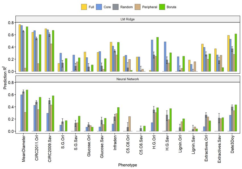
bioRxiv preprint first posted online Jan. 17, 2019; doi: http://dx.doi.org/10.1101/523365. The copyright holder for this preprint
 (which was not peer-reviewed) is the author/funder, who has granted bioRxiv a license to display the preprint in perpetuity.
                                  It is made available under a CC-BY 4.0 International license.

   additive linear model, and a more complex and interactive neural network model in order to
   reflect the mode of action of each type of genes. On one hand, genes that are better predictors
   with an additive model are supposed to have an additive, direct mode of action representing a
   gene that would be downstream in a biological pathway. We expect core genes to display such
   additive behavior, with a high but selectively constrained expression level17,21. On the other
   hand, genes being better predictors with an interactive model are expected to be upstream in
   pathways. We expect peripheral genes to behave interactively, with a lower but relatively more
   variable expression level. With a lower variation, we also expect the core genes to be worse
   predictors for traits than peripheral genes unless larger effects can compensate it but a question
   remains whether it is a matter of trait category or whether the variation is anyway low.
   To answer to these questions and thus empirically test the omnigenic theory, we have
   sequenced the RNA of 459 samples of black poplar (Populus nigra), corresponding to 241
   genotypes, from 11 populations representing the natural distribution of the species across
   Western Europe. We also have for each of these trees phenotypic records for 17 traits, covering
   growth, phenology, physical and chemical properties of wood. They cover two different
   environments where the trees were grown in common gardens, in central France and northern
   Italy. By predicting these traits from our gene expression data, from different gene sets, selected
   based on their topology in networks, we are going to uncover the importance of genes of
   varying centrality in order to test the omnigenic theory.

   Results

   Wood samples, phenotypes, and transcriptomes
   Wood collection and phenotypic data (Table S1) have been previously described24. Further
   details are provided in the methods section. Briefly, we are focusing on 241 genotypes planted
   in 2 common gardens, in Orléans (central France) and Savigliano (northern Italy), and for which
   phenotypic data have been collected. In Orléans, we used 2 clonal trees per genotype to
   sample xylem and cambium during the 2015 growing season for RNA sequencing. We mapped
   the sequencing reads on the Populus trichocarpa transcriptome (v3.0) to obtain gene
   expression data.
   Data collection extended on a 2 weeks period, with varying weather along the days, and
   different operators involved. We did PCA analyses on the cofactors that were presumably
   involved in the experience, to look whether any confounding effect could be identified (Figure
   S1). No clear segregation was found for any of these, except for the ones associated with
   weather. To verify this observation, we used mixed-models to correct effects of all these
   cofactors, with the breedR R package25, and while it properly corrected the environmental
   effects, it also removed information from the data, making prediction quality much poorer than
   without cofactor correction for most of the traits (Figure S2). Since phenotype is a mixture
   between genotype and environment, we supposed that correcting the environment also
   removed natural variation. Further analyses with complex neural network models, expected to
   account more efficiently for interactions with hidden theoretical states, did not show better
   results than additive models. We thus did not favor one particular type of model with

                                                                                                                                    3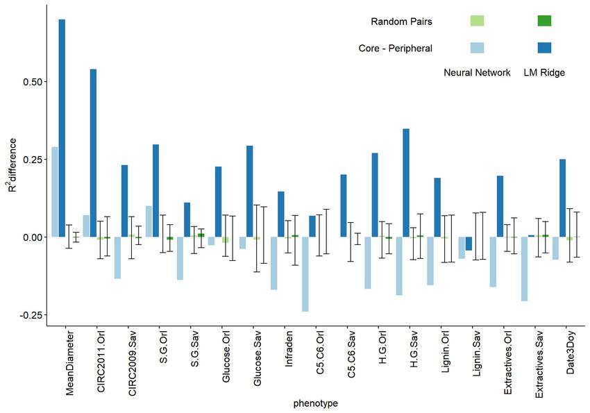
bioRxiv preprint first posted online Jan. 17, 2019; doi: http://dx.doi.org/10.1101/523365. The copyright holder for this preprint
 (which was not peer-reviewed) is the author/funder, who has granted bioRxiv a license to display the preprint in perpetuity.
                                  It is made available under a CC-BY 4.0 International license.

   uncorrected data. Moreover, we did not aim at interpreting the effect of each variable in this
   study but rather at inferring mechanisms from the prediction quality of the different models,
   which might be less prone to confounding effects.
   From the 41,335 transcripts obtained from the mapping, we removed the 1,653 without reads,
   we normalized the read counts, stabilized their variance and transformed the counts of the
   39,682 remaining transcripts to counts per million. Further details are provided in the methods
   section. Hereafter, we refer to this set of 39,682 transcripts as the full gene set (96% of
   annotated transcripts).

   Clustering and network construction
   The classical approach to build a signed scale-free gene expression network is to use the
   weighted correlation network analysis (implemented in WGCNA R package5), using a power
   function on correlations between gene expressions. We chose to use Spearman’s rank
   correlation to avoid any assumption on the linearity of relationships. The scale-free topology
   fitting index (R2) reached a maximum of 0.85 for a soft threshold of 15, yielding a mean
   connectivity of 22.9 (Figure 1A). We detected 25 gene expression modules (Table S2) with
   automatic detection (merging threshold: 0.25, minimum module size: 30, Figure 1B). Spearman
   correlations between 17 traits values and expression, presented in the lower panel of the Figure
   1B below the module membership of each gene, display a structuration when ordered following
   the gene expression tree. The traits themselves are line ordered according to clustering on their
   scaled values to represent their relationships (Figure S3). Interestingly, some patterns in the
   correlation between expression and traits do not follow what we would expect from the similarity
   between traits (3 traits out of 7 with data in both sites). For instance, in the group composed of
   S/G ratios and glucose composition, the patterns were more similar between sites across traits
   than between traits across sites (Figure 1B and S3). Complex shared regulations mediated by
   the environment seem to be in control of these phenotypes, suggesting site-specific genetic
   control. Otherwise, glucose composition in Savigliano, infra-density, and extractives in Orléans
   presented similar patterns, contrarily to what would be expected from the correlations between
   these traits. These results suggest that the comparative analysis of correlations between gene
   expression and between traits allow unraveling underlying links between traits that are not
   obvious from factual phenotypic and genetic correlations between traits.
   To get further insight into the relationships between module composition and traits, we looked at
   the strongest correlations between the best theoretical representative of a gene expression
   module (eigengene) and each trait, in order to identify genes in relevant modules with an
   influence on the trait (Figure 1C). Following a Bonferroni correction of the p-values provided by
   WGCNA, only 72 correlations remained significant (p ≤ 0.05) out of the initial 425 traits by
   modules combinations, and 5 modules were defined as composed of genes not involved in any
   of the traits studied (salmon, greenyellow, brown, lightgreen and darkgrey, Figure S4). In
   significantly correlated modules, gene expression correlation with trait was also significantly
   correlated with centrality in the module (represented by the kME, the correlation with the module
   eigengene), while no correlation was found in poorly correlated modules (Figure 1D, Figure S5).
   In other words, there is a three-way correlation. The genes with the highest kME in a given
   module are the most correlated to the eigengene and, consequently, are also the most

                                                                                                                                    4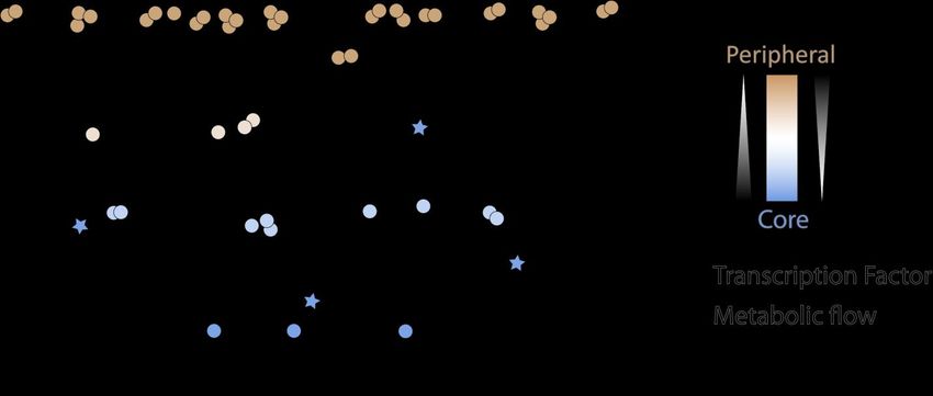
bioRxiv preprint first posted online Jan. 17, 2019; doi: http://dx.doi.org/10.1101/523365. The copyright holder for this preprint
 (which was not peer-reviewed) is the author/funder, who has granted bioRxiv a license to display the preprint in perpetuity.
                                  It is made available under a CC-BY 4.0 International license.

   correlated to those traits with the largest correlation with the module eigengene. Although this is
   somehow expected, it underlines the usefulness of kME as a centrality score to further
   characterize the genes within each module. We thus used this centrality score to define further
   the topological position of our gene expressions in networks. In order to avoid bias in gene
   selection by large groups, we selected the 10% of genes with the highest global absolute scores
   to define the “core genes” group, and the 10% with the lowest global absolute scores to define
   the “peripheral genes” group. Finally, we selected 100 samples of 3968 “random genes” as
   control groups (Figure S6).
   One particular module in the resulting clustering is the grey module. This module typically
   gathers genes with poor membership to any other module. In our case, it is the largest module,
   with 15214 genes (38% of the full set), it gathers the vast majority of genes with very low kME
   (Figure S6) and 99% of the peripheral genes set (Table S4). While it is typically discarded in
   classic clustering studies, its eigengene displays the highest number of significant correlations
   with traits suggesting non-negligible biological roles (Figure 1C, Figure S4). It thus appears
   interesting to use it as a contrasting set for the remaining of the study in the light of the
   omnigenic theory.
   To assess the robustness of WGCNA analysis results, we compared it to a k-means clustering
   (R package coseq25) of the gene expressions (Figure S7A). The distribution of WGCNA and k-
   means’ clusters showed a correlation of 0.42 (Figure S7B). K-means clustering forces groups
   of comparable size, which does not seem biologically credible. Furthermore, the correlations
   between the k-mean modules eigengenes and traits were lower than with WGCNA’s, with a
   poor repartition of the different modules on the first 2 principal component analysis space
   (Figure S7C). We thus preferred WGCNA clustering to k-means clustering for this analysis and
   were quite confident about its robustness given its overall concordance with k-means clustering.

   Boruta gene expression selection
   In addition to previous gene sets building (full, core, random, peripheral), we wanted to have a
   set of genes being relevant for their predictability of the phenotype. Our hypothesis here would
   be that this set is the one that enables the best prediction of a given trait with a limited gene
   number that would be comparable to the other subsets of genes selected on their
   characteristics within the networks. For that purpose, we performed a Boruta (Boruta R
   package26) analysis on the full genes set. This algorithm performs several random forests to
   analyze which gene expression profile is important to predict a phenotype. In the end, a pool of
   637 unique gene expressions was found to be important to predict our phenotypes (Figure S8).
   Traits with the highest number of important genes are related to growth. For the other traits, we
   always have more genes selected when the trait is measured in Orléans compared to
   Savigliano (respective medians of 29 and 17.5). We hypothesize that this is due to the fact that
   RNA extraction was performed on trees in Orléans. One exception to this pattern is the Lignin
   content, that we suspect to be due to a methodological difference between assessments, as
   previously discussed24. On average, genes that were specific to single traits represented 62% of
   selected genes, genes shared across sites for a given trait were 4%, genes shared by trait
   category (growth, phenology, physical, chemical) were 18%, and genes shared among all traits
   were 16%.

                                                                                                                                    5
bioRxiv preprint first posted online Jan. 17, 2019; doi: http://dx.doi.org/10.1101/523365. The copyright holder for this preprint
(which was not peer-reviewed) is the author/funder, who has granted bioRxiv a license to display the preprint in perpetuity.
It is made available under a CC-BY 4.0 International license.
Phenotype prediction with gene expression
For our 5 genes sets (full, core, random, peripheral and Boruta), we trained two classes of
models to predict the phenotypes: an additive linear model (ridge regression) and an interactive
neural networks model. For the former, we used ridge regression to avoid overfitting problems.
For the latter, we chose neural networks as a contemporary machine-learning method, which is
not subjected to dimensionality problems27 and is able to capture interactions without a priori
explicitation between the entries, here gene expressions. Figure 2 and S9 show that for linear
modeling with ridge regression, the best genes set to predict phenotypes was the core gene set,
followed by the full, Boruta, random and peripheral sets (respective median prediction R² over
all traits of 0.33, 0.31, 0.25, 0.18 and 0.16). On the contrary, for neural network modeling, core
genes constituted the worst set by far, followed by a cluster of similarly performing peripheral,
random and Boruta sets (respective median prediction R² over all traits of 0.07, 0.21, 0.22, 0.22).
We have not been able to compute neural network models with the full set as the number of
predictors remains too large to be fitted within a reasonable time on computing clusters. Across
phenotypes (Figure S9), predictions were generally less variable under neural network than
under the ridge regression counterpart (interquartile range mean division by 1.48).
To further investigate the behavior of genes with different positions in networks with respect to
the prediction model used, we computed differences between prediction scores for core and
peripheral gene sets for additive (ridge regression) and interactive (neural network) algorithms
(Figure 3). As a null reference for inference, a randomization strategy involving 100 random
sets of genes was used to infer differences in prediction scores between models due to random
sampling. For this, we computed a total of 4950 differences corresponding to all pairwise
differences, excluding reciprocals and self-comparisons. A positive difference indicates an
advantage of core genes sets over peripherals and, conversely, a negative difference indicates
an advantage of peripheral genes. Except for 4 out of 17 cases, most traits showed a
contrasting behavior of the two alternative algorithms. While most additive ridge regression
models yielded positive scores across traits, the neural network counterpart showed negative
scores. This hints at the fact of different gene actions in the two sets of genes. Indeed, the
former ridge regression models capture mostly additive gene actions, which appeared to be
prominent for core genes. Contrarily, neural network modeling is better suited for revealing gene
interactions, which seem to be inherently associated with peripheral gene functioning. On
average, the neural network has a mean difference of -0.08, showing that they are mainly in
favor of the peripheral genes set. On the opposite, ridge regression models have mean
differences of 0.24, showing that they are predicting a lot better with core genes set. It should be
noted that concording behavior may come from the almost complete inability to predict the
phenotype for a particular trait (a score close to 0 in Figure 2). In most of the cases, the
contrasty pattern between core and peripherals with the two algorithms could not be drawn
exclusively by chance as indicated by the distribution of randomized sets which clearly appears
to be centered on zero (mean differences of -0.002 and 0.0002 for neural network and ridge
regression models respectively).
6bioRxiv preprint first posted online Jan. 17, 2019; doi: http://dx.doi.org/10.1101/523365. The copyright holder for this preprint
(which was not peer-reviewed) is the author/funder, who has granted bioRxiv a license to display the preprint in perpetuity.
It is made available under a CC-BY 4.0 International license.
Heritability and population differentiation of modules
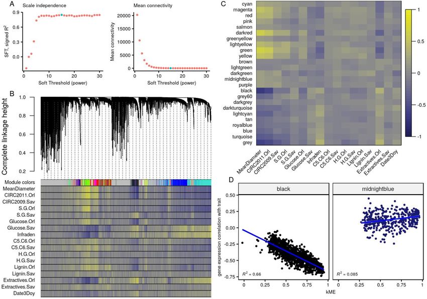
To understand the biological role of core and peripheral genes at population levels, we
computed gene expression level (Figure 4B), several classical population statistics (Figure 4A,
4C, 4E, and 4F) and a contemporaneous equivalent to FST for genome scans (Figure 4D).
Gene expression level, heritability, Qst and coefficient of genetic variation were computed from
gene expression data, while gene diversity and PCadapt scores28 were computed from
polymorphism data (SNP), for more details see the method section.
The extent of heritability for gene expression was higher for random the set than for core and
peripheral genes, the latter having extremely low median heritability (0.04) (Figure 4A). Gene
expression level (Figure 4B) and the extent of population differentiation from expression data
(Figure 4C) tended to be higher in core set than in the other sets, with intermediate levels in the
random set and the lowest levels in the peripheral set. According to PCadapt score (Figure 4D),
core genes showed more evidence of population-specific selection patterns than the other two
sets, with random genes having intermediate levels. Concerning the coefficient of genetic
variation (Figure 4E), there was a clear difference between sets, with core genes displaying a
very low variation, peripheral genes a very high, and random genes intermediate levels. Finally,
there was a small difference in overall gene diversity (Figure 4F) that confirms the differences
observed for CVG computed on gene expression level, peripheral genes being more diverse
than random, and random more diverse than core genes.
Altogether, these statistics showed clear differences between core and peripheral genes: core
genes are highly expressed (Figure 4B), highly differentiated between populations (Figure 4C),
with generally low levels of genetic variation (Figure 4D, 4E, 4F); while peripheral genes are
poorly expressed, poorly differentiated between populations, with generally higher genetic
variations.
Discussion
Omnigenic theory1 states that in gene regulatory networks, highly connected core genes are of
high importance individually but altogether explain only a small part of heritable phenotypic
variation, while peripheral genes, each of low importance and connectivity, altogether explain
the majority of phenotypic variation. This theory, enunciated with human diseases in mind,
needed to be tested with empirical data and broadened to other kingdoms of life.
In order to contribute to the empirical support of the omnigenic theory, we studied in Populus
nigra the role and predictive ability of 2 gene sets, on opposite sides of a gene coexpression
network. We defined core and peripheral genes as the 10% most central and most peripheral
genes respectively according to the outputs of WGCNA analysis. We are aware that this is
somehow an oversimplification, an extreme contrast of an otherwise continuous phenomenon.
Moreover, according to the omnigenic theory, core genes are only a “modest number” and
peripheral genes are the remaining majority of expressed genes. While the choice of the
arbitrary threshold of 10% is based on the Mahler’s definition of core genes8, the fact of
equaling both samples responded to the need for statistical comparativeness between
equivalent samples. Moreover, such contrasting samples represented two conspicuous features
of the distribution of kME (Figure S6), with a thick tail of well-connected genes and a high mass
7bioRxiv preprint first posted online Jan. 17, 2019; doi: http://dx.doi.org/10.1101/523365. The copyright holder for this preprint
(which was not peer-reviewed) is the author/funder, who has granted bioRxiv a license to display the preprint in perpetuity.
It is made available under a CC-BY 4.0 International license.
of poorly connected genes. The outputs of WGCNA analysis on which our gene discrimination is
based provided better results than k-means clustering. It has to be noted that k-means forces
clusters to be of equal size, which could restrain concordance and ultimately does not reflect
biological reality. In addition, we selected these modules on normalized gene counts for which
we only stabilized the variance. No further correction of data could be done without reducing the
prediction signal, thus we have to consider that environmental conditions while showing a low
impact, are not corrected for the present analysis. Despite this environmentally uncorrected data,
clusterings with two methods remain concordant, somehow pinpointing the robustness of the
outcome in gene classification.
On average, core genes were the ones predicting the most efficiently a phenotype, for any trait
category, with an additive model, even if the full set still reaches the highest global prediction R²
(0.77 for the mean sample diameter). This might be expected from the positive and highly
significant relationship observed between gene significance and connectivity within WGCNA
modules displaying a significant correlation with traits. On the other side of networks, peripheral
genes predict better with an interactive model than with an additive one and provide over both
types of models the most stable predictions (interquartile ranges of 0.19 for peripheral, 0.27 for
random, 0.34 for core and Boruta and 0.35 for full set). The information necessary to predict a
phenotype does not seem to be particularly concentrated at any side of the network, but rather
spread over it, as highlighted by the performance of random gene sets. They capitalize enough
information to perform predictions more accurately than an equal number of peripheral genes.
Moreover, prediction with larger peripheral sets (20% and 30% of genes) confirmed that
peripheral genes need to be in a high number to reach high prediction R², as the median
doubled between 10% and 30% sets, but not necessarily with more central genes in the network
as it tended to drop with 40% of genes (Figure S10, median R² of 0.15, 0.23, 0.33 and 0.29
respectively for 10%, 20%, 30% and 40% peripheral gene sets). In that sense, Boruta seems to
be extremely useful to focus on the information that is relevant for prediction. From the 637
genes selected by Boruta, 95 and 22 were core and peripheral genes, respectively. If the
number of core genes within the Boruta set is greater than expected by chance (Fisher’s exact
test p-value < 0.0001), a large majority of Boruta genes still do not belong to this category nor to
the peripheral gene set. Boruta selection proved to be able to select a small number of genes
for all of our phenotypes, allowing for a faster and more precise prediction, with less than one-
sixth of genes compared to the core or peripheral sets, and only 1.6% of the full set, with
predictions being almost as accurate. This makes Boruta an advantageous alternative in
genomic evaluation for breeding to more classic methods (based on the imposition of a priori
constraints for shrinkage or variable selection29) like ridge regression.
Tracking back predictabilities down to particular gene sets is an essential step before being able
to understand the roles of interactivity and connectivity in a gene network underlying the
phenotype. In that sense, the high levels of connectivity shown by core genes do not appear to
be a prerequisite for prediction quality, while these particular genes find better fits in additive
models. Contrarily, peripheral genes, while being poorly connected, display prediction quality
equivalent to random or Boruta sets in interactive models. This pinpoints to an a priori
paradoxical situation in which connectivity and interaction are not necessarily found in the same
gene sets. Here, connectivity refers to the degree of membership of a given gene within a
coexpression network and one should note that this was defined independently from the
8bioRxiv preprint first posted online Jan. 17, 2019; doi: http://dx.doi.org/10.1101/523365. The copyright holder for this preprint
(which was not peer-reviewed) is the author/funder, who has granted bioRxiv a license to display the preprint in perpetuity.
It is made available under a CC-BY 4.0 International license.
phenotype. Interactivity, on the other hand, refers to the way the expression profile of a given
gene is mediated before affecting the phenotype. Such interactivity between gene expressions
is quite different from what is usually referred to as epistasis in the genetics literature, the
interaction effect between alleles from different loci on a given phenotype30, because here the
input is gene expressions instead of allelic polymorphisms. Weather connectivity or interactivity
relates to epistasis is beyond the scope of current work, but clearly deserves further
investigation. In order to clarify this apparent paradox, one hypothetical scenario could be
proposed, following the model schematized in Figure 5. Basically, in this model, a peripheral
gene is located upstream within biological pathways and it produces an essential brick which
can be further modified or complemented by the bricks of subsequent genes downstream. The
peripheral genes that produce essential bricks do it with a low connection to other genes. As we
progress downstream within the pathways, the bricks from peripheral genes suffer a chain of
subsequent modifications due to or controlled by other genes, resulting in an impact on the final
phenotype that can be highly mediated by many intermediaries, appearing as interactors, that
somehow blur the brick’s contribution to the ultimate phenotype. This could explain the
interactive behavior of peripheral genes, as sitting far away from the final phenotype, while
being poorly connected. Core genes, on our schematic model, receive upstream bricks from
many peripheral genes, and their output directly impacts or influence the phenotype. This may
be a reason why core genes while being highly connected, behave additively, as they almost
directly appear to contribute to the phenotype. We have further looked for enrichment in
transcription factors (TFs) within the core and peripheral gene sets and found that TFs were
overrepresented within the core gene set (Fisher’s exact test p-value < 1.10-14), while they were
underrepresented within the peripheral gene set (Fisher’s exact test p-value < 1.10-7). This
leads us to believe that core genes consist in fact of a mixture of highly connected regulators
and genes downstream within biological pathways, which altogether contribute to the metabolic
flow towards phenotypes. Consequently, they would behave additively when predicting a trait,
they could contribute individually to a large proportion of phenotypic variation, and they could,
therefore, suffer “first hand” the selection pressure. Core genes variation levels are low by
comparison to their expression level and they might display distinct optima according to
population structure, as underlined by their higher Qst and PCadapt scores in our data. As they
depend much on other bricks, they have less room for variation, and are somehow “canalized”.
Peripheral genes, on the other hand, are highly variable with lower expression levels. They are
thus the ones by which variations come to the network and propagate downstream. These
observations are consistent with molecular evolution studies, as Jovelin et al.17 showed a
positive correlation between selective constraints and expression level and Fraser & Hirsh23
showed that core genes are more expressed, but less variant compared to their expression.
Finally, Montanucci et al.21 showed a positive correlation between selective constraints and
connectivity, which also echoes in our measures and models.
Our results have brought to the omnigenic theory new insights into the function and behavior of
genes with respect to their position in the network, by an integrative approach combining
predictive and explanatory functions. We also showed that the omnigenic theory holds within
our Poplar dataset, leading us to think that this theory may be more ubiquitous than originally
described. We believe that there is no apparent reason why it would not apply to the entire plant
kingdom and everything that lays in-between humans and poplars on the tree of life. We are
9bioRxiv preprint first posted online Jan. 17, 2019; doi: http://dx.doi.org/10.1101/523365. The copyright holder for this preprint
(which was not peer-reviewed) is the author/funder, who has granted bioRxiv a license to display the preprint in perpetuity.
It is made available under a CC-BY 4.0 International license.
thus making a point here enlarging the omnigenic theory to not only humans as it was first
described but to any living being complex enough to have gene networks.
Methods
Samples collection
As described in previous works24,31, we established in 2008 a partially replicated experiment
with 1160 cloned genotypes, in two contrasting sites in central France (Orléans, ORL) and
northern Italy (Savigliano, SAV). At ORL, the total number of genotypes was of 1,098 while at
SAV there were 815 genotypes. In both sites, the genotypes were replicated 6 times in a
randomized complete block design. At SAV, the trees were pruned at the base after one year of
growth (winter 2008-2009) to remove a potential cutting effect and were subsequently evaluated
for their growth and wood properties during the winter 2010-2011. At ORL, the trees had the
same pruning treatment after two years of growth (winter 2009-2010), and were also
subsequently evaluated for growth and wood properties after two years (winter 2011-2012).
After evaluation, they were pruned again for a new growth cycle. At their fourth year of growth
(2015), 241 genotypes present in two blocks of the French site were selected to perform
sampling for RNA sequencing. In the end, we obtained transcriptomic data from 459 samples.
These 241 genotypes were representative of the natural west European range of P. nigra
through 11 river catchments in 4 countries (Table S3).
We described 14 of the 17 phenotypic traits in a previous work24. Briefly, these traits can be
divided into two categories, growth traits and biochemical traits which were all evaluated on up
to 6 clonal replicates by genotype at each site after two years of growth. The first set is
composed by the circumference of the tree at 1-meter height measured in Savigliano at the end
of 2009 (CIRC2009.Sav) and in Orléans at the end of 2011 (CIRC2011.Orl). The second set is
composed, each time at both sites, of measures of ratios between the different components of
the lignin, p-hydroxyphenyl (H), guaiacyl (G) and syringyl (S) (H.G.Orl, H.G.Sav, S.G.Orl and
S.G.Sav), measures of the total lignin content (Lignin.Orl : measure of the lignin in Orléans,
Lignin.Sav: measure of the lignin in Savigliano), measure of the total glucose (Glucose.Orl and
Glucose.Sav), measure of ratio between 5 and 6 carbon sugars (C5.C6.Orl and C5.C6.Sav) and
measure of the extractives (Extractives.Orl and Extractives.Sav). For each of these traits, we
computed mean values per genotype previously adjusted for microenvironmental effects (block
or spatial position in the field).
The 3 remaining traits were measured in 2015 on the trees harvested for the RNA sequencing
experiment (2 replicates per genotype). They include the mean diameter of the stem section
harvested for RNA sequencing (MeanDiameter), the date of bud flush of the tree in 2015
(Date3Doy) and the basic density of the wood (Infraden). Date of bud flush consisted in a
prediction of the day of the year at which the apical bud of the tree was in stage 3 according to
the scale defined in Dillen et al.32. Predictions were done with a lowess regression from discrete
scores recorded at consecutive dates in the spring of 2015. Wood basic density was measured
on a piece of wood from the stem section harvested for RNA sequencing following the Technical
10bioRxiv preprint first posted online Jan. 17, 2019; doi: http://dx.doi.org/10.1101/523365. The copyright holder for this preprint
(which was not peer-reviewed) is the author/funder, who has granted bioRxiv a license to display the preprint in perpetuity.
It is made available under a CC-BY 4.0 International license.
Association of Pulp and Paper Industry (TAPPI) standard test method T 258 “Basic density and
moisture content of pulpwood”.
Transcriptome data generation
We sampled stem sections of approximately 80 cm long starting at 20 cm above ground and up
to 1 meter in June 2015. The bark was detached from the trunk in order to scratch young
differentiating xylem and cambium tissues using a scalpel. The tissues were immediately
immersed in liquid nitrogen and crudely ground before storage at -80°C pending milling and
RNA extraction. Prior to RNA extraction, the samples were finely milled with a swing mill
(Retsch, Germany) and tungsten beads under cryogenic conditions with liquid nitrogen during
25 seconds (frequency 25 cps/sec). About 100 mg of milled tissue was used to isolate
separately total RNA from xylem and cambium of each tree with RNeasy Plant kit (Qiagen,
France), according to manufacturer’s recommendations. Treatment with DNase I (Qiagen,
France) to ensure elimination of genomic DNA was made during this purification step. RNA was
eluted in RNAse-DNAse free water and quantified with a Nanodrop spectrophotometer. RNA
from xylem and cambium of the same tree were pooled in an equimolar extract (250 ng/µl)
before sending to the sequencing platform.
RNAseq experiment was carried out at the platform POPS (transcriptOmic Platform of Institute
of Plant Sciences - Paris-Saclay) thanks to IG-CNS Illumina Hiseq2000. RNAseq libraries were
constructed using TruSeq_Stranded_mRNA_SamplePrep_Guide_15031047_D protocol
(Illumina®, California, U.S.A.). The RNAseq samples have been sequenced in single-end reads
(SR) with an insert library size of 260 bp and a read length of 100 bases. Images from the
instruments were processed using the manufacturer’s pipeline software to generate FASTQ
sequence files. Ten samples by lane of Hiseq2000 using individually barcoded adapters gave
approximately 20 millions of PE reads per sample. We mapped the reads on the Populus
trichocarpa v3.0 transcriptome with bowtie233, and obtained the read counts for each of the
41,335 transcripts by homemade scripts. Initially, we considered using the genotype mean to
reduce our data volume. However, differences between replicates were not normally distributed,
because of variation in gene expression due to plasticity. We thus could not summarize our data
with their mean, as it would have removed this information and finally we chose to keep
replicates as separate data samples.
Filtering the non-expressed genes, normalization and variance
stabilization
As the sampling ran along 2 weeks, we expected environmental variables to blur the signal. To
understand how our data were impacted, we ran the first analysis, containing a step identifying
the impact of each cofactor and a step correcting confounding effects, with mixed linear models
implemented in the R package breedR25. However, while it was properly correcting the
covariables that seemed to impact our data (environmental effects) when controlling on PCA
spaces, it was also erasing useful information from the data, yielding less accurate prediction
models than without any correction. We thus chose not to perform this correction, and use raw
uncorrected data.
11bioRxiv preprint first posted online Jan. 17, 2019; doi: http://dx.doi.org/10.1101/523365. The copyright holder for this preprint
(which was not peer-reviewed) is the author/funder, who has granted bioRxiv a license to display the preprint in perpetuity.
It is made available under a CC-BY 4.0 International license.
We started cleaning our raw counts data by removing the transcripts with 0 counts for all
individuals. From the original 41,335 genes, 1,653 were thus removed, leaving 39,682 genes
with at least 1 count in at least 1 individual.
After this first filtration, we normalized the raw counts data by Trimmed Mean of M-values (TMM,
edgeR34). As most features are not differentially expressed, this method takes into account the
fact that the total number of reads can be strongly influenced by a low number of features. Then,
we calculated the counts per millions (CPM35).
To stabilize the variance of the CPM data, we computed a log2(n+1) instead of a log2(n+0.5)36
used in a voom analysis35. The reason is that the former avoids negative values, which are
problematic for the rest of the analysis. The resulting data set is called “Full”, these counts are
also shown in Figure 4B.
Hierarchical and k-means clustering
We performed a weighted correlation network analysis with the R package WGCNA5 on our full
RNA sequencing gene set. We followed the classic approach, except that we first ranked our
expression data, to work subsequently with Spearman’s non-parametric correlations and avoid
problems due to linear modeling assumptions. We first chose the soft threshold with the highest
scale-free topology fitting index (R² = 0.85), which is for a power of 15 (connectivity: mean =
22.90, median = 8.94, max = 329, Figure 1A). Then, we used the automatic module detection
(blockwiseModules function) via dynamic tree cutting with a merging threshold of 0.25, a
minimum module size of 30 and bidweight midcorrelations (Figure 1B). All other options were
left to default. This also computes module eigengenes. To order the traits, we clustered their
scaled values with the pvclust R packages37, the Ward agglomerative method (“Ward.D2”) on
correlations (Figure 1B and C, Figure S3). The clustering on euclidian distance results in the
exact same hierarchical tree. Correlations between traits and gene expression or module
eigengenes were computed as Spearman’s rank correlations (Figure 1B lower panel and 1C).
We also performed a k-means clustering with the R package coseq38: considering 10 initial runs,
1000 iterations, without any other data transformation, and for a number of clusters (K) between
2 and 20. At first, it identified a K without strong agreement between the two evaluation
algorithms included in coseq. We computed additional rounds of k-means clustering, between
K-5 and K+5, with 100 initial runs and 10000 iterations, until both evaluation algorithms agreed.
Machine learning
Boruta gene expression selection
In addition to the inconvenience of working with a large number of features (time and power
consumption), most machine learning algorithms perform better when the number of predicting
variables used is kept as low as the optimal set39. We thus performed an all relevant variable
selection40 with the Boruta function26 from the eponym R package, with a 5% p-value threshold,
on the full gene expression set, for each phenotype independently. Then, features that were not
rejected by the algorithm were pooled together, so that all the important genes were in the
selected gene pool.
12bioRxiv preprint first posted online Jan. 17, 2019; doi: http://dx.doi.org/10.1101/523365. The copyright holder for this preprint
(which was not peer-reviewed) is the author/funder, who has granted bioRxiv a license to display the preprint in perpetuity.
It is made available under a CC-BY 4.0 International license.
Models
Both additive linear model (ridge regression) and interactive neural networks models were
computed by the R package h2o41. They both used the gene expression sets as predictors and
one phenotypic trait at a time as a response. Gene sets were split by the function
h2o.splitFrame in 3 sets, a training set, a validation set and a test set, with the respective
proportions of 60%, 20%, 20%. Consequently, to evaluate model quality we used prediction
accuracies reported as R² between observed and predicted values within the test set and using
the function R2 of the R package compositions42.
For linear models, we used the function h2o.glm with default parameters, except 2-folds cross-
validation and alpha set at zero to perform a ridge regression.
Neural networks have the reputation to be able to predict any problem, based on the Universal
approximation theorem43,44. However, this capacity comes at the cost of a very large number of
neurons in one layer, or a reasonable number of neurons per layer in a high number of layers.
Both settings lead to difficult interpretation when very many gene expressions are involved. In
that sense, we chose to keep our models simple, with two layers of a reasonable number of
neurons (see models architectures in Methods). This obviously comes at the price of lower
prediction power. However, we believe that these topologies give us the power to model 2 levels
of interactions between genes (1 level per layer). Furthermore, since both methods yielded
comparable prediction R² (median ridge regression R² = 0.27, mean neural network R² = 0.22),
this complexity seemed appropriate. To find the best models for neural networks, we computed
a random grid for each response. We tested the following hyperparameters: (i) “Rectifier”,
“Tanh”, “RectifierWithDropout” and “TanhWithDropout” activation. (ii) the network structure is
based on the number of genes used as predictors (h). The first layer is composed of h, ⅔h or
⅓h neurons. The second layer has a number of nodes equal or lower to the first one and is also
composed of h, ⅔h or ⅓h neurons. This represents 6 different structures. (iii) Input layer
dropout ratio is 0 or 0.2. (iv) L1 and L2 regularization are comprised between 0 and 1x10⁻⁴, with
steps of 5x10⁻⁶. We performed a random discrete strategy to find the best search criteria,
computing a maximum of 100 models, with a stopping tolerance of 1x10⁻³ and 10 stopping
rounds. Finally, h2o.grid parameters are the following: the algorithm is “deeplearning”, with 10
epochs, 2 fold cross-validation, maximum duty cycle fraction for scoring is 0.025 constraint for a
squared sum of incoming weights per unit is 10. All other parameters have default values. The
best model is selected from the lowest RMSE score within the validation set.
Heritability and Qst Models
A 12k bead chip45 provided 7,896 SNPs in our population. A genomic relationship matrix
between genotypes has been computed with these SNPs by LDAK46, and further split into
between (mean population kinship, ) and within population relationship matrices (kinship kept
only for the members of the same population, all the others are equal to 0, ). These matrices,
associated to design matrices, were used in a mixed linear model to compute an additive
genetic variance between and within populations (equation 1) for the expression of each gene.
In this model, is a gene expression vector across individual trees, is a vector of fixed effects
(overall mean or intercept); and are respectively random effects of populations and
13bioRxiv preprint first posted online Jan. 17, 2019; doi: http://dx.doi.org/10.1101/523365. The copyright holder for this preprint
(which was not peer-reviewed) is the author/funder, who has granted bioRxiv a license to display the preprint in perpetuity.
It is made available under a CC-BY 4.0 International license.
individuals within populations, which follow normal distributions, centered around 0, of variance
and , where and are the between and within population variance component
and and are the between and within population kinship. and are known incidence
matrices between and within populations, relating observations to random effects and . is
the residual component of gene expression, following a normal distribution centered around 0,
of variance , where is the residual variance and is an identity matrix.
(equation 1)
From the between and within population variance components, we can compute heritability (h2,
equation 2) and population differentiation estimates (QST, equation 3) for each gene. To
compute them, we used the function remlf90 from the R package breedR25, with the
Expectation-Maximization method followed by one round with Average-Information algorithm to
compute the standard deviations.
; ;
(equation 2)
(equation 3)
We computed the genetic variation coefficient (CVG) by dividing sums of and by
expression mean, per gene.
Other population statistics
We further used a previously developed bioinformatics pipeline to call SNPs within our RNA
sequences47. Briefly, this pipeline involves classical cleaning and quality control steps, mapping
on the Populus trichocarpa v3.0 reference genome, and SNP calling using the combination of
four different callers. We ended up with a set of 874,923 SNPs having less than 50% of missing
values per genotype. The missing values were further imputed with the software FImpute48. We
validated our genotyping by RNA sequencing approach by comparing the genotype calls with
genotyping previously obtained with an SNP chip on the same individuals45. Genotyping
accuracy based on 3,841 common positions was very high, with a mean value of 0.96 and a
median value of 0.99. The imputed set of SNP was then annotated using Annovar49 in order to
group the SNPs per gene model of P. trichocarpa reference genome. For each SNP, we
computed the overall genetic diversity statistic with the hierfstat R package50 and this statistic
was then averaged by gene model in order to get information on the extent of diversity. We
further computed PCadapt score with the pcadapt R package28 with 8 retained principal
components. Here again, PCadapt scores were then summarized (averaged) by gene model in
order to get information about their potential involvement in adaptation. Based on the principal
component analysis, PCadapt is more powerful to perform genome scans for selection in next-
generation sequencing data than approaches based on FST outliers detection28. We found a
14bioRxiv preprint first posted online Jan. 17, 2019; doi: http://dx.doi.org/10.1101/523365. The copyright holder for this preprint
(which was not peer-reviewed) is the author/funder, who has granted bioRxiv a license to display the preprint in perpetuity.
It is made available under a CC-BY 4.0 International license.
positive correlation between FST and PCadapt score (data not shown), but PCadapt shows
differences between Core, random and peripheral gene sets (Figure 4D) when FST does not.
Transcription factors enrichment analysis
We have tested each of the gene sets (core, peripheral, Boruta, random) for enrichment in
transcription factors, with data coming from the plant TFDB51. We selected in each set
transcripts based on loci, regardless of the transcription factor families sharing different versions
of the gene. Fisher’s exact test was performed with the base R function fisher.test.
Data Availability
This RNAseq project is under submission to the international repository Gene Expression
Omnibus (GEO) from NCBI. All steps of the experiment, from growth conditions to bioinformatic
analyses are detailed in CATdb52 according to the MINSEQE “minimum information about a
high-throughput sequencing experiment”. Raw sequences (fastq) are being deposited in the
Sequence Read Archive (SRA) from NCBI. Information on the studied genotypes is available in
GnpIS53 at the following address:
https://urgi.versailles.inra.fr/gnpis-
core/#form/crops=Forest%20tree&germplasmLists=POPULUS_NIGRA_RNASEQ_PANEL.
Figure Legends
Figure 1 WGCNA analysis of gene expression data. (A) Selection of the soft threshold (green
dot) based on the correlation maximization with scale-free topology (left panel) producing low
mean connectivity (right panel). (B) Gene expression hierarchical clustering dendrogram, based
on the Spearman correlations (top panel), resulting in clusters identified by colors (first line of
the bottom panel). Spearman correlations between gene expressions and traits are represented
as color bands on the other lines of the bottom panel, from highly negative correlations (dark
blue) to highly positive correlations (light yellow), according to the scale displayed in panel C. (C)
Spearman correlation between eigengenes (the best theoretical representative of a gene
expression module) of modules identified in the previous panel and traits, again on a dark blue
(highly negative) to light yellow (highly positive) scale. (D) Focus on two modules from the
previous graph, representing the correlations between gene expression correlation with mean
sample diameter and centrality in the module. These two panels represent the strongest (left
panel, black module, R2 = 0.66) and the weakest (right panel, midnightblue module, R2 = 0.09)
correlations with the corresponding trait.
Figure 2 Predictions scores on test sets (R² on the y axis) for the 2 algorithms (LM Ridge, top
panel; neural network, bottom panel) for each phenotypic trait (on the x axis). The color of each
bar represents the gene set that has been used for the prediction. Intervals for the random set
represent the first and third quartiles of the distribution of the 100 different realizations, while the
height of the bar corresponds to the median.
15bioRxiv preprint first posted online Jan. 17, 2019; doi: http://dx.doi.org/10.1101/523365. The copyright holder for this preprint
(which was not peer-reviewed) is the author/funder, who has granted bioRxiv a license to display the preprint in perpetuity.
It is made available under a CC-BY 4.0 International license.
Figure 3 Difference of prediction scores (on the y-axis) between the core and peripheral gene
sets (in blue) or between random sets (in green), for additive (LM Ridge in saturated colors) and
interactive (neural network in faded colors) algorithms, for the different traits (on the x-axis). For
the random pairs, error bars represent the first and third quartiles of the differences between
pairs of randomized sets and the bar corresponds to the median.
Figure 4 (a) Heritability h², (b) gene expression (in counts per million), (c) differentiation QST, (d)
PCadapt score, (e) genetic variation coefficient CVG and (f) overall gene diversity Ht violin plots
for each of the core (in blue), random (in grey) and peripheral (in brown) gene sets. ns: p > 0.05,
*: pbioRxiv preprint first posted online Jan. 17, 2019; doi: http://dx.doi.org/10.1101/523365. The copyright holder for this preprint
(which was not peer-reviewed) is the author/funder, who has granted bioRxiv a license to display the preprint in perpetuity.
It is made available under a CC-BY 4.0 International license.
144 (2008).
12. Rausher, M. D., Miller, R. E. & Tiffin, P. Patterns of evolutionary rate variation among genes
of the anthocyanin biosynthetic pathway. Mol. Biol. Evol. 16, 266–274 (1999).
13. Riley, R. M., Jin, W. & Gibson, G. Contrasting selection pressures on components of the
Ras-mediated signal transduction pathway in Drosophila. Mol. Ecol. 12, 1315–1323 (2003).
14. Han, M. et al. Evolutionary rate patterns of genes involved in the Drosophila Toll and Imd
signaling pathway. BMC Evol. Biol. 13, 245 (2013).
15. Song, X., Jin, P., Qin, S., Chen, L. & Ma, F. The evolution and origin of animal Toll-like
receptor signaling pathway revealed by network-level molecular evolutionary analyses.
PLoS One 7, e51657 (2012).
16. Wu, X. et al. The evolutionary rate variation among genes of HOG-signaling pathway in
yeast genomes. Biol. Direct 5, 46 (2010).
17. Jovelin, R. & Phillips, P. C. Expression level drives the pattern of selective constraints along
the insulin/Tor signal transduction pathway in Caenorhabditis. Genome Biol. Evol. 3, 715–
722 (2011).
18. Duret, L. & Mouchiroud, D. Determinants of substitution rates in mammalian genes:
expression pattern affects selection intensity but not mutation rate. Mol. Biol. Evol. 17, 68–
74 (2000).
19. Pál, C., Papp, B. & Hurst, L. D. Highly expressed genes in yeast evolve slowly. Genetics
158, 927–931 (2001).
20. Drummond, D. A., Bloom, J. D., Adami, C., Wilke, C. O. & Arnold, F. H. Why highly
expressed proteins evolve slowly. Proc. Natl. Acad. Sci. U. S. A. 102, 14338–14343 (2005).
21. Montanucci, L., Laayouni, H., Dall’Olio, G. M. & Bertranpetit, J. Molecular evolution and
network-level analysis of the N-glycosylation metabolic pathway across primates. Mol. Biol.
Evol. 28, 813–823 (2011).
22. Bloom, J. D. & Adami, C. Evolutionary rate depends on number of protein-protein
interactions independently of gene expression level: response. BMC Evol Biol 4, 14 (2004).
23. Fraser, H. B. & Hirsh, A. E. Evolutionary rate depends on number of protein-protein
interactions independently of gene expression level. BMC Evol Biol 4, 13 (2004).
24. Gebreselassie, M. N. et al. Near-infrared spectroscopy enables the genetic analysis of
chemical properties in a large set of wood samples from Populus nigra (L.) natural
populations. Ind. Crops Prod. 107, 159–171 (2017).
25. Muñoz, F. & Sanchez-Rodriguez, L. breedR: Statistical Methods for Forest Genetic
Resources Analysts. (2018).
26. Kursa, M. B. & Rudnicki, W. R. Feature Selection with the Boruta Package. J. Stat. Softw.
36, 1–13 (2010).
27. González-Recio, O., Rosa, G. J. M. & Gianola, D. Machine learning methods and predictive
ability metrics for genome-wide prediction of complex traits. Livest. Sci. 166, 217–231
(2014).
28. Luu, K., Bazin, E. & Blum, M. G. B. pcadapt: an R package to perform genome scans for
selection based on principal component analysis. Mol. Ecol. Resour. 17, 67–77 (2017).
29. de Los Campos, G., Hickey, J. M., Pong-Wong, R., Daetwyler, H. D. & Calus, M. P. L.
Whole-genome regression and prediction methods applied to plant and animal breeding.
Genetics 193, 327–345 (2013).
30. Cordell, H. J. Epistasis: what it means, what it doesn’t mean, and statistical methods to
detect it in humans. Hum. Mol. Genet. 11, 2463–2468 (2002).
31. Guet, J. et al. Genetic variation for leaf morphology, leaf structure and leaf carbon isotope
discrimination in European populations of black poplar (Populus nigra L.). Tree Physiol. 35,
850–863 (2015).
32. Dillen, S. Y., Marron, N., Sabatti, M., Ceulemans, R. & Bastien, C. Relationships among
productivity determinants in two hybrid poplar families grown during three years at two
17You can also read