Lossless Multi-Scale Constitutive Elastic Relations with Artificial Intelligence
←
→
Page content transcription
If your browser does not render page correctly, please read the page content below
Lossless Multi-Scale Constitutive Elastic Relations
                                                                                 with Artificial Intelligence

                                                             Jaber Rezaei Mianroodi1,∗ , Shahed Rezaei2 , Nima H. Siboni3 ,
                                                                                          Bai-Xiang Xu2 , Dierk Raabe1
                                                                                     1
                                                                                         Microstructure Physics and Alloy Design,
arXiv:2108.02837v1 [cond-mat.mtrl-sci] 5 Aug 2021

                                                                       Max-Planck-Institut für Eisenforschung, Düsseldorf, Germany
                                                              2
                                                                  Mechanics of Functional Materials Division, Institute of Materials Science,

                                                                          Technische Universität Darmstadt, Darmstadt, Germany
                                                                         3
                                                                             DeepMetis, Lohmühlenstraße 65, 12435 Berlin, Germany
                                                                                 ∗
                                                                                     Corresponding Author j.mianroodi@mpie.de

                                                                                                   August 9, 2021

                                                                                                       Abstract

                                                          The elastic properties of materials derive from their electronic and atomic nature.
                                                      However, simulating bulk materials fully at these scales is not feasible, so that typi-
                                                      cally homogenized continuum descriptions are used instead. A seamless and lossless
                                                      transition of the constitutive description of the elastic response of materials between
                                                      these two scales has been so far elusive. Here we show how this problem can be over-
                                                      come by using Artificial Intelligence (AI). A Convolutional Neural Network (CNN)
                                                      model is trained, by taking the structure image of a nanoporous material as input
                                                      and the corresponding elasticity tensor, calculated from Molecular Statics (MS), as
                                                      output. Trained with the atomistic data, the CNN model captures the size- and pore-
                                                      dependency of the material’s elastic properties which, on the physics side, can stem
                                                      from surfaces and non-local effects. Such effects are often ignored in upscaling from
                                                      atomistic to classical continuum theory. To demonstrate the accuracy and the effi-
                                                      ciency of the trained CNN model, a Finite Element Method (FEM) based result of an
                                                      elastically deformed nanoporous beam equipped with the CNN as constitutive law is
                                                      compared with that by a full atomistic simulation. The good agreement between the
                                                      atomistic simulations and the FEM-AI combination for a system with size and surface
                                                      effects establishes a new lossless scale bridging approach to such problems. The trained
                                                      CNN model deviates from the atomistic result by 9.6% for porosity scenarios of up
                                                      to 90% but it is about 230 times faster than the MS calculation and does not require
                                                      to change simulation methods between different scales. The efficiency of the CNN
                                                      evaluation together with the preservation of important atomistic effects makes the
                                                      trained model an effective atomistically-informed constitutive model for macroscopic
                                                      simulations of nanoporous materials, optimization of nano-structures, and solving of
                                                      inverse problems.

                                                    Keywords— Atomistic simulations, Molecular statics, Aluminium, Machine learning, Porosity,

                                                                                                           1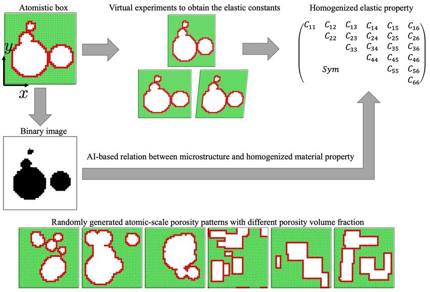
Artificial intelligence, Anisotropic elasticity tensor.

1     Introduction

The laws of mechanics are rather well established at the macroscopic continuum scale. This applies
particularly for the linear relationship between stress and strain, such as cast in Hooke’s linear
elasticity law nearly 350 years ago. The material-specific properties are represented through the
elastic stiffness modulus, which in three dimensions is a 4th order tensor. However, when leaving
the idealized continuum description of bodies and zooming into their underlying micro-cosmos,
also referred to as microstructure, a very complex landscape emerges which is characterized by a
wide range of structural features and defects. Some of these microstructure features do not alter
the macroscopic stiffness substantially or only in a rather modest and linear fashion, but others
lead to more drastic changes of the elastic response. This applies particularly to the porosity of
the material, a property which refers to the volume fraction, dispersion and connectivity of the
open volume. In such cases the elastic modulus of the representative volume element of a material
can be altered quite substantially. The relationship between porosity and elastic stiffness as well
as its size-dependence across several scales is of importance for a number of material classes. One
example is bone, where diseases such as osteoporosis lead to loss in bone mass through the highly
dispersed micro-architectural deterioration of bone tissue, an effect which entails decay in elastic
stiffness and bone fragility [1]. A direct relationship between porosity across all size scales and the
resulting stiffness and strength also applies for wood, which is currently gaining rapid momentum
as sustainable construction material [2]. Another example is the development of nano- and micro-
porosity during the direct reduction of iron ores [3]. This effect leads to gradual loss in stiffness
which has severe consequences for the design of corresponding direct reduction and fluidized bed
reactors, a field of utmost relevance for the carbon free reduction of metal oxides.

    Also many functional materials have a nano- or micro-porous structure, such as aerogels, many
catalysts or supercapacitors [4]. Most of these materials do not only fulfill their respective func-
tional role but must at the same time bear mechanical loads, where the elastic stiffness assumes
a central role in their property portfolio. Another field where porosity and stiffness are closely
connected is the domain of additive manufacturing which plays an increasing role in digital manu-
facturing. Most parts cannot be manufactured to 100% mass density so that better understanding
of corresponding stiffness effects due to the inherited porosity is an important aspect [5].

    A size-dependency of the elastic properties is particularly expected when it comes to nanoporous
materials which are attributed to the competition between surface and bulk energies, especially
at smaller scales [6–8]. Classical models of elasticity should be extended correspondingly through
the incorporation of surface elasticity models [9–11]. The reader is referred to [12–15], and the
references therein for an overview of surface effects in case of elasticity and plasticity. One effective
approach is to utilize interface finite elements on the surface of models that represent nanostruc-
tured materials. The latter method requires explicit input of the surface tension constants and
surface elastic parameters in the case of surface elasticity. Also, such surface elements induce
implementation and computational complications [13, 16]. A size effect is also predicted in the
torsion and bending of open-cell foams or lattices, where slender specimens appear stiffer than
expected. Such size effect can be predicted by Cosserat elasticity (also known as micropolar elas-
ticity). Such models are sensitive to strain gradients and introduce a characteristic length into
the constitutive formulations which, however, require complex experimental characterization to
identify the required constitutive parameters (see also [17]). When it comes to the mechanical

                                                    2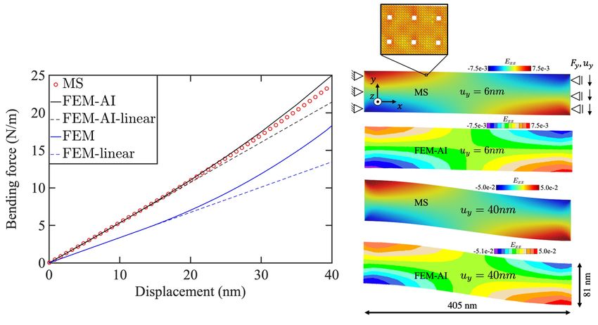
and topological homogenization of such materials, further extensions are required to calibrate an
effective generalized continuum model that is applicable across several scales [18–20].

   A straightforward way to calculate the true elastic stiffness of nanoporous materials is conduct-
ing atomistic calculations which naturally consider all relevant porosity and surface tension features
arising form it [21, 22]. However, this is not feasible when targeting the mechanical description
of larger parts, revealing the typical scale-dilemma often encountered in computational materials
science. This problem is also often referred to as the multi-scale and multi-physics challenge in
materials mechanics [23].

   The multi-scale modeling strategy requires, on one hand, accurate and predictive simulation
at lower scales taking various physical phenomena into account, and on the other hand, efficient
methodologies to transfer the information between the scales. In the available scale-bridging tech-
niques, there is usually a trade-off between the amount of information preserved in the up-scaling
and the associated computational costs. One way to establish this micro-macro coupling is to
make use of Artificial Intelligence (AI). Machine Learning (ML) seems to provide a promising
approach for an efficient scale-bridging. As mentioned, the properties of a material depend to a
large extend on a wide cosmos of defects, which is also referred to as nano- and microstructure,
and on the mutual interaction among all these features. The high-dimensional and tensorial inter-
action among these multiple nano- and microstructure features makes the required dimensionality
reduction of the scale transfer problem much more complex than just transferring the chemical
composition and some overall geometrical factors from one scale to another. Empirical descriptors
that could be predefined to capture and reflect some of these features and their change upon scale
transitions are usually unknown and difficult to determine. Instead, in most cases, there are more
complex and sometimes even weakly understood interactions hidden inside the material’s nano-
and microstructure. Therefore, image-based AI methods can be valuable tools for the study of
microstructure-dependent structure-property relations [24, 25] in general (due to the many effects
and phenomena involved) and specifically for scale-bridging structure-property calculations (where
even some of the physics for adequate coarse-graining have not been resolved yet). In [26], a sum-
mary is provided over recent advances in the application of AI techniques for numerical modeling of
various types of materials such as metals, polymers, ceramics and composites. Owing to their high
efficiency, allowing very fast calculations, AI techniques open up new efficient strategies to optimize
and drastically accelerate structure-property calculations of future advanced engineering materials
and structures [27]. These approaches could also help to discover scale bridging phenomena that
had so far remained elusive, hidden behind the enormous chemical and structural complexity of
modern engineering materials. Peng et al. [28] discussed the state of the art of combining ML
and multi-scale modeling in various applications. Bock et al. [29] reviewed successful applications
of ML and statistical learning methodologies in the field of continuum materials mechanics. They
concluded that simulation-based data mining in combination with ML tools provide exceptional
opportunities for identification of fundamental interrelations within materials.

   Different ML strategies have been investigated for modeling at different length scales. Wang
and Sun [30] replaced the up-scaling procedure through an offline homogenization procedure by
utilizing a sub-scale simulations to generate a database to train material models for geological
materials. Xue et al. [31] proposed a data-driven multi-scale computational scheme to capture the
non-linear mechanical behavior of cellular meta-materials. See also [32] for similar studies. Kumar
et al. [33] introduced a ML technique for the inverse design of meta-materials which is able to
generate functionally graded cellular structures with tailored anisotropic stiffness. Wang et al. [34]
developed a data-driven method for an efficient multi-scale topology optimization. The application

                                                  3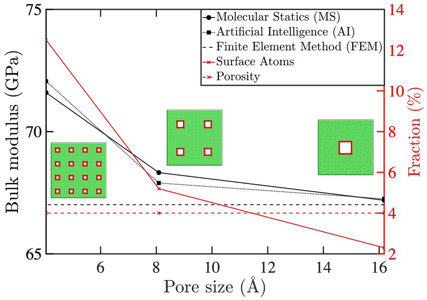
of ML has also been extended to more complicated material behavior including plasticity [35, 36].
Readers are referred to [25, 37] for similar studies in different application fields. It is worth to
mention that the ML approaches can be applied to construct a direct solver for the usually well-
known Partial Differential Equations (PDEs) out of massive data sets. Samaniego et al. [38]
explored deep neural networks as an option to approximate the solution of the underlying PDEs.
Raissi et al. [39] introduced a physics-informed neural network which takes into account any given
laws described by general non-linear PDEs. The authors demonstrated the effectiveness of the
proposed framework through application to classical problems in fluids, quantum mechanics and
reaction–diffusion systems. Yang et al. [40] employed conditional generative adversarial neural
network to predict stress and strain fields directly from the material microstructure geometry.
Wang et al. [41] introduced a genomic flow network and a mosaic flow predictor to estimate
the solution of Laplace and Navier-Stokes equations in domains of unseen shapes and boundary
conditions. Pandey et al. [42] proposed a ML based surrogate model for predicting spatially
resolved crystal orientation evolution under uniaxial tensile loading. It is also important to make
sure that the trained network prediction satisfies the fundamental physical and thermodynamics
laws [43] or fulfills the objectivity and possible material symmetry conditions [44].

   In this scientific context, Convolutional Neural Networks (CNNs) are employed extensively to
extract material property-structure relationships based on microstructure images [45, 46]. Cecen et
al. [47] employed a CNN to link a three-dimensional microstructure to its effective (homogenized)
properties. The authors showed that the trained CNN is able to learn physically interpretable
microstructure features and accurately predict desired properties. Rao and Liu [48] proposed a
three-dimensional deep CNN to predict the anisotropic effective material properties for representa-
tive volume elements with random inclusions. The dataset generated by a computational homog-
enization approach was used for training the network. They concluded that the trained networks
can predict unseen data, indicating that the network is capable of capturing the microstructural
features of the system and could produce an accurate prediction of the effective anisotropic stiff-
ness tensor. Recently, Mianroodi et al. [24] applied a U-Net approach to predict stress fields in
geometrically complex and heterogeneous non-linear elasto-plastic material systems. It was shown
that the U-Net-based prediction of the stress fields in such a highly non-linear system was about
8000 times faster than that obtained by a typical spectral solver (e.g. [49]). Interestingly, the
U-Net was also capable to reproduce the stress distribution in geometries topologically far from
those that had been used for training.

   Although the body of literature on multiple possible and promising applications of ML in mate-
rial science is growing fast, a general approach for transferring constitutive relations directly from
atomistic to continuum scale is missing. In the current work, we use Mishin’s interatomic potential
for Al [50] to calculate the elasticity tensor for large sets of randomly generated nanoporous struc-
tures. A CNN is then trained using the topology data (stored as images of the atomic structure)
and the calculated elasticity tensor components as reference data set. Once the network is trained,
it is evaluated in terms of several test cases, showing its ability to capture full atomistic details
(such as pore surface effects) while being orders of magnitude faster than the atomistic calculations.
The efficiency of the AI-based method coupled with an accurate description of the atomistic scale
effects on the material’s elastic constitutive response, results in a lossless scale-bridging approach.
The preparation of the training data from the atomistic calculations is presented in Section 2. The
architecture and training of the CNN is discussed in Section 3. The performance and accuracy of
the trained CNN is evaluated in Section 4. Finally, the paper is concluded in Section 5 with a
discussion and outlook.

                                                  4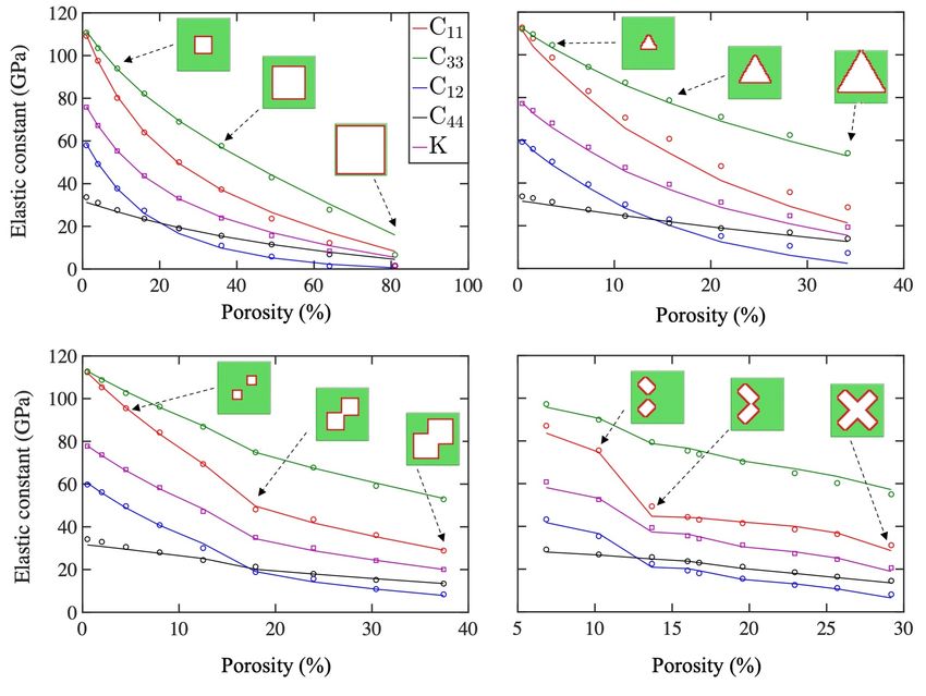
2     Workflow and Preparation of Atomistic Data

An important step in training a neural network consists in obtaining an accurate and diverse
set of training data. In this work we use Molecular Statics (MS) to calculate the anisotropic
elastic constants of face centered cubic (fcc) aluminum with randomly distributed porosity. The
Mishin embedded atom potential [50] in conjunction with LAMMPS [51] is employed to calculate
the elastic constants. The fully periodic simulation box size is set to (Lx , Ly , Lz ) = (20, 20, 3)a0
where a0 = 4.05 Å is the lattice constant. The schematics of the method along with exemplary
nanoporous structures are shown in Figure 1.

Figure 1: Schematic of the workflow for the elasticity tensor calculation from molecu-
lar statics and corresponding image-based artificial intelligence prediction. In this figure
and in the others to follow, green and red correspond to the atoms with fcc lattice and
unknown (surface) structures, respectively, identified using common neighbor analysis as
implemented in the freeware visualization and analysis package Ovito [52]. In the binary
image generated from the corresponding atomisitc structure, the pore area is indicated in
black while the solid material region in white. Selected examples of the randomly generated
circular and rectangular pore structures are shown in the bottom row.

    The box is periodic in all directions, representing an infinite array of the pore structure inside
the box. Initially the box is filled with N = 4800 Al atoms. Then a random target porosity volume
fraction in range of (0, 90) percent is selected. The porosity volume fraction is defined as

                                               N −n
                                          p=        × 100,                                          (1)
                                                N
where n and N are the number of atoms in the porous and non-porous (completely filled) boxes,
respectively. Note that p is 0% and 100% in the case of a full simulation box (n = N ) and empty
space (n = 0), respectively. Once the target porosity volume fraction, for brevity referred to
as porosity from here on, is chosen, a number of pores with random shape, size, and position are
created by removing atoms from the box until the porosity (p) is above or equal the target porosity.

                                                  5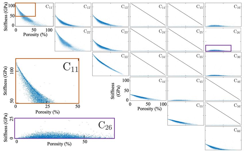
The pores are defined as geometrical regions with circular or rectangular shapes with random
attributes. To avoid unstable structures, which would complicate the automated MS calculations,
all pores are constrained to have minimum distance of 0.4nm from the box boundaries. This will
ensure non-zero stiffness in all directions and avoids crumbling structures due to open pores and
disconnected parts.

    After the desired porosity volume fraction is reached, the atomistic sample is relaxed to zero
stress state using a combination of conjugate gradient and FIRE (a damped dynamics method
described in [53]) algorithm. Once all stress components (including shear components) are zero,
the elastic stiffness calculation is performed using the script in LAMMPS which works by distorting
the system infinitesimally in different directions and calculating the change of stress, thereby,
measuring the components of the elasticity tensor.

    In addition to the porosity volume fraction introduced in (1), we introduce an atomistic measure
for quantifying the pore dispersion
                                            ns
                                         d=       × 100,                                    (2)
                                           N −n
where ns is the total number of surface atoms, identified using common neighbour analysis [52].
Note that for a given porosity volume fraction p, i.e. constant N − n, the dispersion d is maximised
when the pore surface area, i.e. number of atoms at the surface ns , is maximised. This typically
translates into dispersing the same pore volume fraction into smaller average pore sizes. Note that
other quantification measures of porous media such as percolation and dispersion are also available.
In the current case, since the structures are randomly generated, at each porosity volume fraction
level, we generate many structures with different percolation and dispersion.

    Without loss of generality, we consider first 2D pore structures in the x-y plane, while along
the z direction, no structure variation is assumed, i.e. mimicking an extruded nanostructure. The
scheme presented should also work for general 3D nanoporous structures, except that the training
of the CNN model becomes computationally more expensive. Thus, only variations in x-y plane
are important here, resulting in the possibility of representing the atomic positions and topology
of the pores by a single image. The image is created after full stress relaxation and serves as the
input for the CNN. The corresponding outputs are the components of the elasticity tensor.

    Two datasets with circular and rectangular pore shapes are generated, respectively. Each
dataset consists of about 10,000 cases, resulting in total 20,000 sets of input image and output
elastic constants. Exemplary pore structures selected from each of the datasets are shown in the
bottom row of Figure 1.

3     Network Architecture and Training

Using ML has become ubiquitous in material science (see Refs. [54–65] for a review). These
applications include accelerated material discovery [66–69], efficient interatomic potential devel-
opment [70–73], feature identification from complex patterns that have relevance for materials
performance [74–78], or facilitating predictive simulations which solve macroscopic (non-linear)
partial differential equation systems [24, 39, 79]. This has the potential to revolutionize continuum-
based simulations of materials, allowing a substantial enhancement in the modeling of systems and
topologies with high complexity. Macroscopic simulations (with or without AI) require homoge-
nized and averaged material property descriptors, e.g. elastic constants and yield strength, as their
inputs. In a multi-scale approach these macroscopic properties are estimated using microscopic
simulations like molecular dynamics or ab initio calculations [80]. Interestingly, ML has been also

                                                  6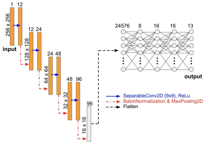
applied to replace (at least partially) the expensive microscopic simulations. These efforts include
replacing the computationally costly interatomic ab initio force calculations by a neural network
[81], or replacing the trajectory prediction using graph neural networks [82]. A common feature of
these ML solutions is that the atomistic coordinates are transferred to the network as its input.

   Unlike these approaches, in our case we use the image of the microstructure as the input and
predict the aggregated effect of the interatomic forces and the arrangements of the atoms. In
this respect, our work is similar to the approach introduced in [83] where 2D X-ray images of the
microstructure are used as the input and macroscopic material properties like porosity, specific
surface area, and average pore size of each image are computed. CNN models of homogenized
mechanical properties have been trained in relation to mesoscopic microstructure with multiple
phases [45–47], whereby the classical continuum theory was applied to each phase and for the
evaluation of the effective properties. Our approach differs fundamentally from these CNN models
in the sense that we apply atomistic calculations to obtain the property which automatically map
the surface effects, namely, the elastic stiffness changes resulting from the surface reconstructions
of the many atoms surrounding the pores, and thus can recapitulate the resultant size dependency.

3.1    Neural network architecture

Neural networks vary in their basic neural units, the arrangement of these units in the layers and
their connectivity, the character of the loss functions (e.g in terms of the quantification of the
deviations of the predicted values relative to the reference values in the training data), and the
’reductionist’ spirit of the network design (e.g. see Refs. [84–86]). We build our neural network
under the assumption that the macroscopic properties can be obtained as a non-linear function of
the coarse-grained local information. In other words, the network extracts the local information,
coarse grains it, and finally passes this information to a (learnable) non-linear function. This is
reflected in the architecture of our neural network, as shown in Figure 2.

   Given that (i) the input to our network is an image and (ii) the first step is to extract the
local information, we use convolutional layers which are the most widely used neural network
architecture for image processing [87]. We apply, successively, a number of convolutional layers
where each layer is accompanied by a coarse-graining step which is implemented by a max pooling
operation. The convolutional layer is commonly coded in the form of a simple matrix (of much
lower rank compared to the image size). This matrix, which is commonly referred to as the kernel,
is sequentially slid across the image and multiplied at each sequential position with a subset of
the input array such that the output enhances certain topological pattern features such as edges,
corners, gradients, etc. As a rule of thumb, including more kernels in the design of the network
leads to a better performance of the network; simply put, the network then has a larger potential
for detecting features. As mentioned before, candidate quantities for these features could be
gradients, edges, etc. Note that these features are not hard-coded. Instead, the network learns
by itself what the important features are. The process of learning the elements of these kernels
is as follows. The elements of this matrix are initially set to be random numbers but during the
training phase, the neural network learns an appropriate set of values for these elements such that
(together with the rest of the network) the prediction error is minimized. To enable the network
to obtain different types of (necessary) information, a number of kernels are used. After feature
extraction and coarse-graining, the most coarse-grained information is mapped to the homogenized
properties via a number of dense layers, which is essentially a non-linear transfer function.

   The neural network that we utilized here is very similar to the encoder part of the U-Net

                                                 7
Figure 2: The artificial neural network architecture used in this work consists of a convo-
lutional part (left) and dense layers (right). The input is a 256×256 pixel binary image
and the output is a set of 13 scalar values of the elasticity tensor.
architecture [85], which has shown to be a good candidate for capturing solutions to solid mechanics
PDEs [24]. Generally speaking, the encoders map the information from one space to another, where
the second space is smaller in its dimensions. Later, this condensed information is passed to the
decoder whose task is to map the information from the low dimensional space back to a high
dimensional space. In the case of the U-Net, the high-dimensional input is an image (which is for
example a RGB image showing an object). This image is transferred to the encoder and condensed
to a much smaller image. Then, the condensed data is sent to the decoder which creates an image
with the size of the original image (which is for example a mask indicating the positions of that
object in the original image). In the current approach, we replace the decoder by a non-linear
function which maps the encoded representation to the scalar output values (the elasticity tensor
components) which we are interested in.
3.2 Neural network training
In the current implementation, for the convolutional layers a kernel of size k × k with k = 20 is
used. The kernel size used here is considerably larger (i.e. ' 6 times) than that used in the original
CNN design. The rationale behind using a larger size is to capture more non-local effects. The
number of channels progressively increases from one channel input data to the embedded space
which has 96 channels as shown in Figure 2. After that, we use five dense layers in conjunction
with a Rectified Linear Unit (ReLU) activation function which are accompanied by the last dense
layer with no activation function (i.e. the identity activation function). The training is performed
by minimizing the loss function which measures the mean squared difference between the predicted
and atomistically calculated values across all the 13 outputs. Note that, as it will be explained in
the next section, only 13 components of the full elasticity tensor are independent in the current case.
This error minimization is done using the ADAM optimizer [88] which is a stochastic first-order
gradient-based method. The parameters of the ADAM optimizer are set to β1 = 0.9, β2 = 0.999,
8 = 10−7 , and a learning rate within the range [1, 2] × 10−4 . We use random samples in batches
of size 128 for the gradient estimation, and continue training for 1000 epochs. In each epoch, the
complete training dataset is used. The data is divided into training and validation sets as explained
in the next section.
4 Results
4.1 Atomistic results
From the 20,000 randomly generated structures and the resultant elasticity tensors, only those
with positive definite elasticity tensors are selected. Since the pore structures are random, in
some cases, the geometry is not stable, leading to incorrect elasticity calculations. After filtering
these unacceptable cases, 18,172 samples with physically meaningful input and output data are
used for training the CNN. All of these data is visualized in Figure 3. Note that the randomly
shuffled dataset is divided into training and validation (test) subsets with sizes of 17,172 and 1000,
respectively.
Figure 3: Elasticity tensor components for 18,172 atomistic boxes with randomly generated
pore structure as a function of the box porosity volume fraction, defined in (1). All the
plots (except the zoomed versions of C11 and C26 at the bottom left) have the same range
in horizontal (porosity) and vertical (stiffness) axes.
As observed in Figure 3, the dispersion of the data is increasing as the porosity is increased.
This is expected as there are more random ways to create the same porosity volume fraction when
it it increased. Also note that more of the cases in high porosity regions are filtered out due to
the instability of the generated structures. Therefore, the number of data for structure regimes
with higher porosity is lower compared to those with low porosity. As explained in Section 2,
randomly generated structures with higher porosity fractions are often unstable and cause issues
for the automated elasticity tensor calculations. Therefore, there is an unbalanced distribution
9of data at different porosity levels. As it will be shown later, this results in a reduced prediction
accuracy for the higher porosity levels with lower number of training data.
As it is shown in Figure 3, only 13 components are non-zero (within tolerance of 10−3 GPa),
instead of 21 for a general elasticity tensor. This is due to the assumed 2D variation of the
pore structures and translates to the introduction of a symmetry-breaking effect, rendering the
structure response monoclinic (rather than cubic) (with a plane of symmetry) [89]. Note that the
Voigt notation, i.e. (11, 22, 33, 23, 13, 12) → (1, 2, 3, 4, 5, 6) is employed. Therefore the CNN has 13
scalar outputs for one input image as summarized above. The magnified views of the C11 and C26
plots are also shown in Figure 3. As apparent for the C11 plot, there is a high density of points
along a curve from 0% porosity up to about 20%. This high point density portion of the curve is
visible as a line shadow in this region which seemingly disappears for porosity values above 20%.
This can be due to the percolation threshold, i.e. as the porosity volume fraction increases, at a
certain threshold (which highly depends on the structure) most of the pores will be connected to
each other increasing the dispersion in the data.
For the C26 elastic constant, the maximum dispersion of the data is around 20-25% porosity
while the data points are closer to each other for porosity values around 0% and above 50%. A
similar trend is visible for other components such as C16 and C36 . This could be also related to
the percolation threshold discussed above.
4.2 Benchmarking AI predictions
The overall mean square error of the trained network on the test dataset is about 7.6GPa, which
corresponds to about 9.6% of the equivalent bulk modulus of single crystalline Al. However, besides
the 1000 cases of the atomistic data reserved for the test dataset as explained above, we also look
into a few special cases here to evaluate the performance of the network. Note that these cases
were neither part of the training nor the test dataset.
4.2.1 Size effects
One major difference between continuum mechanics and atomic systems is the non-local nature of
the interactions in the latter. Due to the quantum-mechanical nature of their electronic bonding,
atoms (particularly in metals) interact over a wide distance (where in simulations a cutoff radius
is usually defined) as opposed to local material models used in classical solid mechanics. This
non-local interaction leads to the distinction between atoms at a free surface with broken neighbor
bonds and atoms in the perfect bulk fcc lattice where all bonds are saturated. As systems become
smaller, the ratio of atoms at surfaces to the atoms in the bulk increases (see red solid line in
Figure 4). To demonstrate the performance of the trained CNN, we investigate the size effect
dependency of the effective bulk modulus of a system with a pore and compare the results from
the MS simulations, as well as classical continuum mechanics solved using the FEM in conjunction
with a linear elastic constitutive law, without any phenomenological size effect considered. Note
that the bulk modulus in this work is the equivalent bulk modulus of single crystalline Al with
arbitrary pore structure.
To this end, three boxes with square shaped pores are considered as shown in Figure 4. In
all cases the simulation size and orientation is the same as explained in Section 2. The pore in
simulation box on the right hand side of the figure has the edge length of Lx /5, resulting in a
porosity volume fraction of p = 4%. In all other steps, the edge length of the pore is divided by
10Figure 4: Effective bulk modulus (black) as a function of pore dispersion in three simulation
boxes shown. Classical linear elastic continuum mechanics (solved by FEM, dashed black)
shows no size effect, while atomistic calculations (solid black) and AI predictions (dotted
black) show a significant size effect. Note that the pore volume fraction (dashed red) is
constant for all three cases while the fraction of atoms that are located at the inner surfaces
of the pores (solid red) increases as the pores get smaller, an effect which leads to a stiffer
response.
two (area reduced by a factor of four) while the number of pores are quadrupled. Therefore, N − n
and the porosity volume fraction, see (1), of the three boxes remains unchanged (dashed red line
in the figure) while dispersion parameter d, see (2), is increased from 56.3% to 125.0% and 300.0%
in the three cases, as the pore sizes become smaller.
The same input structure is fed to the trained CNN and the predicted bulk modulus is plotted in
Figure 4 as solid black squares. As observed, the CNN prediction captures the pore size dependency
of the bulk modulus with good agreement compared to the MS calculations. Note that the trained
CNN is predicting the 13 components of the elasticity tensor as discussed above. The effective
bulk modulus is calculated using
dP ∆P
K = −V ≈ −V , (3)
dV ∆V
where V , ∆P = (S11 + S22 + S33 )/3 and ∆V = V (1 + E11 )(1 + E22 )(1 + E33 ) − V are the volume,
and the differential of the hydrostatic pressure and volume, respectively. Stress S and strain E are
related through the elastic relation S = CE. Under the small deformation assumption and with
initially undeformed / stress-free conditions the differentials can be approximated as
∆V = 3V, ∆P = (S11 + S22 + S33 )/3, (4)
where E11 = E22 = E33 = is assumed. Combining (3) and (4), we get
1
K≈− (S11 + S22 + S33 ). (5)
9
The bulk modulus is then obtained employing (5) and applying an equal triaxial strain state on
the system. Such displacement boundary conditions were applied for both, the MS and the linear
elastic FEM calculations. In the FEM case, the solid phase is equipped with the anisotropic elastic
property of single crystalline Al while the pore has zero stiffness. Note that in all the simulations
11and results reported in this paper, we work with single crystalline material and a full anisotropic
elasticity model. Homogenized polycrystalline properties could be extracted from these for any
given grain structure [90].
The classical continuum prediction for the single crystal bulk elastic modulus of this system
is size independent (dashed black line in Figure 4) with a value of 67.0GPa. However, the MS
calculations show a size effect in the bulk modulus with an increase from 67.2 to 71.6GPa (6.5%
increase) as the pores get smaller from 16.1 to 4.0 Å (solid black line in the figure). This is correctly
captured by the trained CNN with a relative error of about 0.6% compared to the MS-based values.
4.2.2 Porosity and connectivity
Here, we systematically evaluate the CNN-based prediction of various components of the single
crystal elasticity tensor against the MS results for special cases shown in Figure 5.
Figure 5: Atomistic calculations (solid lines) and AI predictions (markers) for selected
components of elasticity tensor and effective single crystal bulk modulus for cases with
simple geometries of one square pore (top left), triangular pore (top right), two square
pores (bottom left) and two rectangular pores (bottom right).
As seen in Figure 5 top left for the case of a square-shaped pore, the agreement between MS
(solid lines) and CNN prediction (marked points) is excellent. For example, considering the C33
results, the relative error starts from 0.6% for the smallest pore size and increases to 8.7% for the
second largest pore (before the last one). The CNN prediction deviates about 58% from atomistic
calculations in the last point of the comparison at a very large porosity of 81%. The deviation is
attributed mainly to the reduced number of training data provided at such high porosity levels as
discussed in Section 4.1. Furthermore, as explained above, the training data exclude all pores that
12were positioned closer than 4Å to the boundary of the box, which explains the larger deviation
between the AI prediction and MS results at the highest porosity volume fraction in this case.
The CNN prediction also shows a relatively good agreement with the MS results in the system
with a triangular pore as shown in the right top panel of Figure 5. Although the error of 1.1% for
the initial microstructure is increased to 34% for the largest pore, the network still captures the
important trend in the results. The higher error compared to square-shaped pores in the previous
case is probably due to the fact that no triangular or similar shaped pores were included in the
randomly generated training dataset, as opposed to random circular and rectangular shaped pores.
In the case of two growing squares in the bottom left panel of this figure, an interesting change
in the slope of the plot (in particular for C11 ) is visible. This change in the slope is due to the
two squares reaching each other and overlapping after this point. The change in slope is correctly
captured by the CNN prediction signifying the effectiveness of the trained network for including
effects of topology, particularly of pore percolation. Since the maximum porosity in this case is up
to 37%, the CNN prediction agrees much better (compared to previous cases) with the MS results
with a maximum relative error of 2.2%. A similar test for two rectangular pores of increasing size
has been performed with the results shown at the bottom right panel of Figure 5. Similar to the
previous case, the overlapping of the two rectangles leads to changes in the slope of the plots. The
agreement between CNN predictions and MS results is quite good with maximum error of about
5.0%. The changes in the slope of the plots indicate the effect of connectivity of the pores on the
data, which seems to be captured by the CNN correctly.
Next, we study a case of a vertically growing pore with both, CNN and MS calculations.
As shown in Figure 6, this case is analogous to a crack growth, where depending on the crack
orientation, a strong asymmetry for the elasticity components is expected. Some components of
the elasticity tensor drastically decrease (e.g. C11 ) while others remain almost constant (e.g. C44 )
or decrease with a lower rate (e.g. C33 ), as the vertical pore length increases.
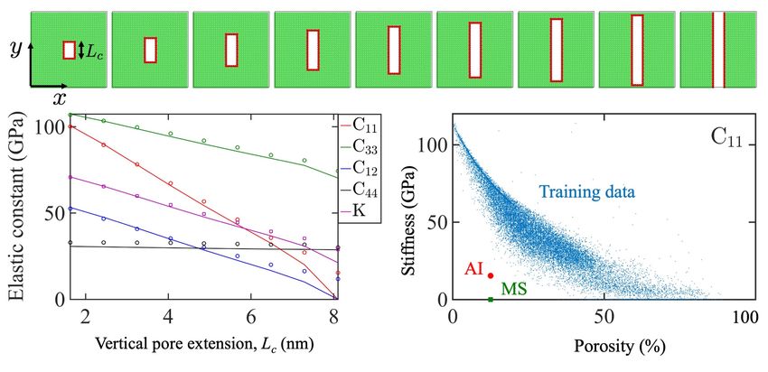
Figure 6: Top row: Simulation boxes with vertically growing rectangular pore of length
Lc . Bottom-left: MS calculation (solid lines) and AI prediction (markers) for single crystal
elasticity tensor components in a vertically growing rectangular pore as a function of Lc .
Bottom-right: The C11 training data as well as the MS calculation and AI prediction for
the case of Lc = 8.0nm (bottom right).
According to Figure 6 bottom left, the agreement between MS and CNN-based prediction is
13apparent for smaller pore lengths. The trained model is also sensitive to the pore orientation and
captures the stiffness degradation correctly. As the pore becomes longer in the vertical direction
and therefore gets closer to the box boundaries, the error of the CNN prediction increases. In the
limit of a fully separated box (Lc = 8.0nm), as expected, the MS prediction for C11 provides a
complete loss in stiffness, whereas the AI prediction for this case is C11 = 15.4GPa. This case, as
shown in Figure 6 at the bottom right, is completely out of the range of the training data. However,
the AI prediction, although associated with high error, is also out of the training data range and
qualitatively points in the correct direction. For better evaluation of fully grown pores (which
could for instance mimic cracks or delamination features) and separated boxes, the training data
should include such cases. However, in this work, we only focus on cases with non-zero stiffness
and non-fractured boxes.
4.3 Lossless multi-scale modeling
The CNN prediction of the elasticity tensor has been incorporated in an FEM model as a continuum
scale constitutive law to simulate bending of a nanoporous beam. The beam dimensions are
(lx , ly , lz ) = (405.0, 81.0, 1.2)nm with free surfaces in x and y and periodic boundary condition
along the z axis. The left side of the beam is fixed in all directions while the right side is displaced
step-wise in −y direction up to |uy | = 40nm. The atomistically modeled beam has square shaped
pores with side length and spacing of 0.40 and 1.46nm, respectively, and consists of 2,304,480
atoms. Note that the porosity of the beam corresponds to the smallest pore size studied in Section
4.2.1.
Figure 7: Comparison of force per unit length in z of the beam as a function of displacement
in y (left) based on fully atomistic simulations (red markers) and a large deformation finite
element calculation equipped with the AI-based constitutive elastic relation (black line),
as well as the FEM model with size independent constitutive relation (blue line). The
dashed lines are the system response ignoring the large deformation effects. Strain fields
calculated at two different beam deflections of 6nm and 40nm based on MS and FEM-AI
are shown on the right side.
The same beam geometry is simulated by FEM in conjunction with a full anisotropic elasticity
14tensor predicted by AI for this porosity. The beam is then loaded in a geometrically non-linear
FEM simulation up to |uy | = 40nm. The resulting force-displacement curve agrees well with
the results obtained from the full atomistic simulations. Note that, as shown in Section 4.2.1,
this pore size introduces a significant surface/size effect compared to a continuum pore. As seen
from the results, using the AI-based constitutive model, seems to correctly transfer the mechanical
behaviour of the system from the atomistic scale into a continuum model.
The results of the FEM simulations obtained by using Hooke’s law for the linear elastic con-
stitutive response, i.e. without the AI-based size-dependent elastic model, are shown in Figure 7
left as blue curve, for the same pore distribution. As it is seen here, ignoring size dependency of
the elastic stiffness introduces a significant error in the predicted bending behaviour of the beam.
For example, at |uy | = 20 nm, MS and FEM-AI both predict a bending force of 11.0 N/m while
the size-independent FEM calculation predicts a bending force of 7.0 N/m. Note that the sur-
face effects increase the stiffness of the system as shown in Figure 4. Therefore, as expected, the
atomistic simulation and the FEM simulation in conjunction with the AI-based elastic constitutive
model predict higher forces for the same beam displacement compared to the FEM with no surface
effects. The deviation (about 5.2% at |uy | = 40 nm) between the MS and the FEM-AI simula-
tions for larger displacements is partly due to the increased pore deformation and its effect on the
elasticity tensor. The FEM-AI case at the moment does not update the pore shape to reevaluate
the elasticity tensor during the loading. However, this will be straightforward to implement and
expected to resolve the deviation at larger deformation values as well.
For a better comparison and to emphasize the potential of the AI-based multi-scaling consti-
tutive modeling capability, we compared the computational time required for different approaches
as well as different steps of the training in Table 1. In the first row, the required computational
times for training the network (as explained in section 3.1 with the data in section 2) is listed.
Next, the computation time for one elasticity tensor calculation with MS and AI is compared. The
bottom two rows of the table list the computation times required for the nanoporous beam bending
simulations as discussed above.
Time (sec) System
AI training 2.0 × 10⁵ (∼2 days) NVIDIA Tesla P4 GPU
Elasticity tensor calculation
MS 101 Intel i7-860 2.80 GHz (single core)
AI 0.43 Intel i7-860 2.80 GHz (single core)
Nanoporous beam bending test
MS 2.03 × 10⁶ (∼23 days) Intel Xeon 6150 2.70 GHz (×2, 36 cores)
FEM-AI 35.5 1 CPU (averaged over 10 simulations)
Table 1: Computational time for training the network and a single elasticity tensor calcu-
lation with MS and AI, as well as the beam bending test (bottom two rows) with different
approaches.
As listed in Table 1, although the training time of the CNN is about two days, the evaluation of
the trained network for the prediction of the full elasticity tensor is about 230 times faster than the
MS calculations. This significant speed-up in elasticity tensor calculation will benefit FEM-MS-
based multi-scale modeling, where each integration point of the elements in the continuum scale
15FEM model is represented by an atomistic simulation box. Since in the current simple example of
a uniform pore structure in the beam exposed to a bending load, an on-the-fly evaluation of the
AI-based elasticity tensor was not necessary, the FEM method with the AI-calculated constitutive
relation (FEM-AI) is significantly (about five orders of magnitude in this particular example) faster
than the full atomistic (MS) calculation, while still capturing important size effects as shown in
Figure 7. Note that the speed-up in this case highly depends on the problem complexity and
the numbers reported in the lower part of the Table 1 are only representative of the current case
and presented here as a first point of reference. The main speed-up reported is the calculation of
the fully anisotropic elasticity tensor with AI as compared to the time-consuming MS methods.
It should be also considered in this context that the elastic response is the most simple, fast
and straightforward mechanical response feature to predict in such atomistic calculations. When
addressing more complex size-dependent nanostructural features, such as for instance inelastic
response of materials under load, atomistic calculations are computationally much more costly, so
that corresponding AI approximations of the size dependence (or other types of) underlying and
homogenized constitutive response might profit even much more from such methods.
5 Conclusions and Outlook
In this work, we show a lossless and efficient approach to use AI techniques to derive constitutive
laws for multi-scale modeling of materials with complex nanostructures. Two ideas are presented,
namely, (1) using computations at the atomistic scale and transfer the information to the continuum
level to arrive at physics-motivated model parameters without any ad-hoc assumptions or empirical
approximations. (2) A Convolutional Neural Network (CNN) is used to directly relate the image
of an arbitrary complicated material structure to its homogenized properties. More specifically, we
focused on obtaining the anisotropic elastic properties of a nanoporous aluminum single crystal,
as a reference model substance, which can be well simulated by atomistic methods. Random
porous structures are generated and their homogenized anisotropic elasticity tensor is calculated
using Molecular Statics (MS). We show that all the non-local effects arising from the physical
nature of the material’s response at the atomistic scale (i.e. surface and size effects) are captured
in this step. The complex pore structure and the details of the atomistic reconstructions at
the pore surfaces, necessitates a neural network design that can detect the local properties and
aggregate that information for use at a coarse-grained scale. The convolutional neural networks
are one of the few appropriate candidates to achieve this flow of information. The trained CNN
confirms this by adequately predicting the elasticity tensor of completely new porous structures
which were not included in the training set. Finally, the proposed methodology is applied to
a simple structural problem of a beam under bending load. We show that by using a Finite
Element Method (FEM) simulation in conjunction with the AI-based constitutive relations, one
can efficiently and accurately predict the material’s structural behavior (in the elastic regime, with
full size dependence) with the accuracy of full atomistic simulations. We also observed that the
trained AI can predict anisotropic elastic properties about 230 times faster compared to performing
corresponding MS calculations. Based on the latter observation, one can also conclude that such
materials-related accelerated and lossless AI-based multi-scale modeling will have at least the same
amount of speed-up compared to a conventional hierarchical multi-scale simulation combining FEM
and MS.
Although the performance of the proposed approach using the investigated dataset is significant,
there is room for further improvements. As an example, it would be interesting to enrich the current
16training data set by including more cases with much higher porosity, including zero stiffness cases
as well as open-cell topologies. Finally, instead of training the symmetric part of the stiffness
tensor, one can try to predict the Cholesky factor of a tangent stiffness matrix to impose a weak
convexity on the strain energy function [91]. The latter point is specifically interesting when it
comes to non-linear material behavior.
The present work opens up many opportunities for efficient and yet accurate inverse design
strategies. For future work, the current methodology can be extended to study similar engineer-
ing materials with complex inherent porosity features such as metamaterials, biological matter,
additively manufactured materials, batteries or foams [92–94]. Investigations should be done to
compare the introduced AI-based model with more advanced non-local elasticity models such as
micropolar [95] or peridynamics [96] theory. Furthermore, instead of finding the symmetric part
of the stiffness tensor as an output, one can focus on obtaining the total scalar elastic energy as
a function of the given deformation gradient. In this manner, one can also derive physics-based
material non-linearities for hyperelastic response. The proposed approach may also be extended to
perform studies on arbitrary (nano-) composite volume elements with various phases. As a result,
one can obtain not only the mechanical properties (e.g stiffness tensor) but also other physical
properties such as effective thermal conductivity or the mobility of chemical species in such com-
plex types of matter. The reported collection of data can also help to understand how the porosity
with an arbitrary shape influences the overall stiffness. Such information could be further used
for developing damage models at coarse-grained scales. In other words, the structure dependent
change in the stiffness tensor, for instance due to creep porosity or micro-fracture patterns, can
be used to represent the level of damage or degradation due to the change in porosity within each
material point. Finally, other fundamental and essential properties such as direction-dependent
fracture energy [97] may be extracted from atomistic simulations. The anisotropic fracture en-
ergy together with anisotropic elastic properties can be directly passed to macroscopic phase-field
damage models at larger scales for conducting efficient calculations based on atomistic data.
Acknowledgements
We thank Prof. Bob Svendsen for fruitful discussions during this work.
References
[1] Ström, O. et al. Osteoporosis: burden, health care provision and opportunities in the EU.
Archives of Osteoporosis 6, 59–155 (2011).
[2] Wimmers, G. Wood: a construction material for tall buildings. Nature Reviews Materials 2,
17051 (2017).
[3] Kim, S.-H. et al. Influence of microstructure and atomic-scale chemistry on the direct reduction
of iron ore with hydrogen at 700°c. Acta Materialia 212, 116933 (2021).
[4] Chowdhury, A. H., Salam, N., Debnath, R., Islam, S. M. & Saha, T. Chapter 8 - design
and fabrication of porous nanostructures and their applications. In Beeran Pottathara, Y.,
Thomas, S., Kalarikkal, N., Grohens, Y. & Kokol, V. (eds.) Nanomaterials Synthesis, Micro
and Nano Technologies, 265–294 (Elsevier, 2019).
17[5] Zhang, B., Liu, S. & Shin, Y. C. In-process monitoring of porosity during laser additive
manufacturing process. Additive Manufacturing 28, 497–505 (2019).
[6] Lucchetta, A., Brach, S. & Kondo, D. Effects of particles size on the overall strength of
nanocomposites: Molecular dynamics simulations and theoretical modeling. Mechanics Re-
search Communications 114, 103669 (2021).
[7] Wang, J., Duan, H., Huang, Z. & Karihaloo, B. A scaling law for properties of nano-structured
materials. Proceedings of the Royal Society A: Mathematical, Physical and Engineering Sci-
ences 462, 1355–1363 (2006).
[8] Chen, S. & Yao, Y. Elastic Theory of Nanomaterials Based on Surface-Energy Density.
Journal of Applied Mechanics 81 (2014).
[9] Shuttleworth, R. The surface tension of solids. Proceedings of the Physical Society. Section A
63, 444–457 (1950).
[10] Gurtin, M. E. & Ian Murdoch, A. A continuum theory of elastic material surfaces. Archive
for Rational Mechanics and Analysis 57, 291–323 (1975).
[11] Javili, A., McBride, A., Steinmann, P. & Reddy, B. D. A unified computational framework for
bulk and surface elasticity theory: a curvilinear-coordinate-based finite element methodology.
Computational Mechanics 54, 745–762 (2014).
[12] Li, Z. & Steinmann, P. Rve-based studies on the coupled effects of void size and void shape
on yield behavior and void growth at micron scales. International Journal of Plasticity 22,
1195–1216 (2006).
[13] Firooz, S., Steinmann, P. & Javili, A. Homogenization of Composites With Extended General
Interfaces: Comprehensive Review and Unified Modeling. Applied Mechanics Reviews 73
(2021).
[14] Wei, G., Shouwen, Y. & Ganyun, H. Finite element characterization of the size-dependent
mechanical behaviour in nanosystems. Nanotechnology 17, 1118–1122 (2006).
[15] Stein, P., Zhao, Y. & Xu, B.-X. Effects of surface tension and electrochemical reactions in
li-ion battery electrode nanoparticles. Journal of Power Sources 332, 154–169 (2016).
[16] Rezaei, S., Mianroodi, J. R., Khaledi, K. & Reese, S. A nonlocal method for modeling
interfaces: Numerical simulation of decohesion and sliding at grain boundaries. Computer
Methods in Applied Mechanics and Engineering 362, 112836 (2020).
[17] Rueger, Z. & Lakes, R. S. Experimental Study of Elastic Constants of a Dense Foam with
Weak Cosserat Coupling. Journal of Elasticity 137, 101–115 (2019).
[18] Forest, S. & Trinh, D. Generalized continua and non-homogeneous boundary conditions
in homogenisation methods. ZAMM - Journal of Applied Mathematics and Mechanics /
Zeitschrift für Angewandte Mathematik und Mechanik 91, 90–109 (2011).
[19] Kouznetsova, V., Geers, M. G. D. & Brekelmans, W. A. M. Multi-scale constitutive modelling
of heterogeneous materials with a gradient-enhanced computational homogenization scheme.
International Journal for Numerical Methods in Engineering 54, 1235–1260 (2002).
18[20] Geers, M., Kouznetsova, V. G. & Brekelmans, W. A. M. Multiscale first-order and second-
order computational homogenization of microstructures towards continua. International Jour-
nal for Multiscale Computational Engineering 1 (2003).
[21] Guillotte, M., Godet, J. & Pizzagalli, L. A fully molecular dynamics-based method for mod-
eling nanoporous gold. Computational Materials Science 161, 135–142 (2019).
[22] Patil, S. P., Rege, A., Sagardas, Itskov, M. & Markert, B. Mechanics of nanostructured
porous silica aerogel resulting from molecular dynamics simulations. The Journal of Physical
Chemistry B 121, 5660–5668 (2017).
[23] van der Giessen, E. et al. Roadmap on multiscale materials modeling. Modelling and Simu-
lation in Materials Science and Engineering 28, 043001 (2020).
[24] Mianroodi, J. R., H. Siboni, N. & Raabe, D. Teaching solid mechanics to artificial intelli-
gence—a fast solver for heterogeneous materials. npj Computational Materials 7, 99 (2021).
[25] Lin, B., Bai, Y. & Xu, B.-X. Data-driven microstructure sensitivity study of fibrous paper
materials. Materials & Design 197, 109193 (2021).
[26] Huang, J. S., Liew, J. X., Ademiloye, A. S. & Liew, K. M. Artificial Intelligence in Materials
Modeling and Design. Archives of Computational Methods in Engineering 28, 3399–3413
(2021).
[27] Salehi, H. & Burgueño, R. Emerging artificial intelligence methods in structural engineering.
Engineering Structures 171, 170–189 (2018).
[28] Peng, G. C. Y. et al. Multiscale Modeling Meets Machine Learning: What Can We Learn?
Archives of Computational Methods in Engineering 28, 1017–1037 (2021).
[29] Bock, F. E. et al. A review of the application of machine learning and data mining approaches
in continuum materials mechanics. Frontiers in Materials 6, 110 (2019).
[30] Wang, K. & Sun, W. A multiscale multi-permeability poroplasticity model linked by recursive
homogenizations and deep learning. Computer Methods in Applied Mechanics and Engineering
334, 337–380 (2018).
[31] Xue, T. et al. A data-driven computational scheme for the nonlinear mechanical properties
of cellular mechanical metamaterials under large deformation. Soft Matter 16, 7524–7534
(2020).
[32] Le, B. A., Yvonnet, J. & He, Q.-C. Computational homogenization of nonlinear elastic ma-
terials using neural networks. International Journal for Numerical Methods in Engineering
104, 1061–1084 (2015).
[33] Kumar, S., Tan, S., Zheng, L. & Kochmann, D. M. Inverse-designed spinodoid metamaterials.
npj Computational Materials 6, 110 (2019).
[34] Wang, L., Tao, S., Zhu, P. & Chen, W. Data-Driven Topology Optimization With Multiclass
Microstructures Using Latent Variable Gaussian Process. Journal of Mechanical Design 143
(2020). 031708.
[35] Settgast, C., Hütter, G., Kuna, M. & Abendroth, M. A hybrid approach to simulate the
homogenized irreversible elastic–plastic deformations and damage of foams by neural networks.
International Journal of Plasticity 126, 102624 (2020).
19You can also read