On the multi-wavelength variability of Mrk 110: Two components acting at different timescales

Page created by Ronald Miller
 
CONTINUE READING
On the multi-wavelength variability of Mrk 110: Two components acting at different timescales
MNRAS 000, 1–19 (2021)                                               Preprint 13 April 2021              Compiled using MNRAS LATEX style file v3.0

                                              On the multi-wavelength variability of Mrk 110: Two components
                                              acting at different timescales

                                              F. M. Vincentelli1? , I. McHardy 1 , E. M. Cackett2 , A. J. Barth3 , K. Horne4 ,
                                              M. Goad5 , K. Korista6 , J. Gelbord7 , W. Brandt8,9,10 , R. Edelson11 , J. A. Miller2 ,
                                              M. Pahari12 , B.M. Peterson12,13 , T. Schmidt14 , R. D. Baldi15,1 , E. Breedt16 ,
                                              J. V. Hernández Santisteban4 , E. Romero-Colmenero17,18 , M. Ward19 ,
arXiv:2104.04530v1 [astro-ph.HE] 9 Apr 2021

                                              D.
                                              1
                                                  R. A. Williams20
                                                Department of Physics and Astronomy, University of Southampton, SO17 1BJ, UK
                                              2 Wayne   State University, Department of Physics & Astronomy, 666 W Hancock St, Detroit, MI 48201, USA
                                              3 Department of Physics and Astronomy, 4129 Frederick Reines Hall, University of California, Irvine, CA, 92697-4575, USA
                                              4 SUPA Physics and Astronomy, University of St. Andrews, North Haugh, KY16 9SS, UK
                                              5 School of Physics and Astronomy, University of Leicester, Leicester, LE1 7RH, UK
                                              6 Department of Physics, Western Michigan University, 1120 Everett Tower, Kalamazoo, MI 49008-5252, USA
                                              7 Spectral Sciences Inc., 4 Fourth Avenue, Burlington, MA 01803, USA
                                              8 Department of Astronomy and Astrophysics, The Pennsylvania State University, 525 Davey Lab, University Park, PA 16802, USA
                                              9 Institute for Gravitation and the Cosmos, The Pennsylvania State University, University Park, PA 16802, USA
                                              10 Department of Physics, 104 Davey Lab, The Pennsylvania State University, University Park, PA 16802, USA
                                              11 Department of Astronomy, University of Maryland, College Park, MD 20742-2421, USA
                                              12 Department of Physics, Indian Institute of Technology, Hyderabad 502285, India
                                              13 Center for Cosmology and AstroParticle Physics; The Ohio State University; 192 West Woodruff Ave., Columbus, OH 43210, USA
                                              14 Department of Physics and Astronomy, University of California, Los Angeles, CA 90095-1547, USA
                                              15 INAF - Istituto di Radioastronomia, Via P. Gobetti 101, I-40129 Bologna, Italy
                                              16 Institute of Astronomy, University of Cambridge, Madingley Road, Cambridge, CB3 0HA, UK
                                              17 South African Astronomical Observatory, P.O Box 9, Observatory 7935, Cape Town, South Africa
                                              18 Southern African Large Telescope Foundation, P.O Box 9, Observatory 7935, Cape Town, South Africa
                                              19 Centre for Extragalactic Astronomy, Department of Physics, University of Durham, South Road, Durham, DH1 3LE, UK
                                              20 Jodrell Bank Centre for Astrophysics, School of Physics and Astronomy,The University of Manchester, Manchester, M13 9PL, UK

                                              Accepted XXX. Received YYY; in original form ZZZ

                                                                                       ABSTRACT
                                                                                       We present the first intensive continuum reverberation mapping study of the high accretion-
                                                                                       rate Seyfert galaxy Mrk 110. The source was monitored almost daily for more than 200 days
                                                                                       with the Swift X-ray and UV/optical telescopes, supported by ground-based observations from
                                                                                       Las Cumbres Observatory, the Liverpool Telescope, and the Zowada Observatory, thus ex-
                                                                                       tending the wavelength coverage to 9100 Å. Mrk 110 was found to be significantly variable
                                                                                       at all wavebands. Analysis of the intraband lags reveals two different behaviours, depending
                                                                                       on the timescale. On timescales shorter than 10 days the lags, relative to the shortest UV
                                                                                       waveband (∼ 1928 Å), increase with increasing wavelength up to a maximum of ∼ 2d lag for
                                                                                       the longest waveband (∼ 9100 Å), consistent with the expectation from disc reverberation. On
                                                                                       longer timescales, however, the g-band lags the Swift BAT hard X-rays by ∼ 10 days, with the
                                                                                       z-band lagging the g-band by a similar amount, which cannot be explained in terms of sim-
                                                                                       ple reprocessing from the accretion disc. We interpret this result as an interplay between the
                                                                                       emission from the accretion disc and diffuse continuum radiation from the broad line region.
                                                                                       Key words: accretion, accretion disc — galaxies: Seyfert — black hole physics — X-rays:
                                                                                       galaxies — galaxies: individual: Mrk 110

                                                                                                                            1   INTRODUCTION
                                              ?   E-mail:F.M.Vincentelli@soton.ac.uk                                        Despite decades of observations across almost all of the accessi-
                                                                                                                            ble electromagnetic spectrum, and their impact in galaxy evolution
                                              © 2021 The Authors
2     F. M. Vincentelli et. al
(e.g., Ferrarese & Merritt 2000; Gebhardt et al. 2000; Marconi et al.    addition, almost all observations show that the X-rays lead the UV
2004), many aspects of active galactic nuclei (AGN) are still poorly     by considerably longer than would be expected purely on the basis
understood. Whilst it is clear that the origin of emission from AGN      of direct reprocessing by an accretion disc. Finally, long-timescale
is fundamentally the result of accretion of matter onto supermas-        lightcurves sometimes have shown in the UV/optical trends which
sive black holes (SMBHs; 106 − 109 M ) at the centre of galaxies         are not paralleled in the X-rays, implying an additional source of
(Lynden-Bell 1969; Rees 1984; Event Horizon Telescope Collab-            UV/optical variability (e.g. Breedt et al. 2009; McHardy et al. 2014;
oration et al. 2019), understanding their detailed inner geometry        Hernández Santisteban et al. 2020; Kammoun et al. 2021b).
remains challenging (Padovani et al. 2017).                                    A number of possible solutions to these problems have been
      Most of the AGN luminosity is released as thermal radiation        proposed. The over-large discs might be explained if the discs are
from an optically thick, geometrically thin accretion disc which         clumpy (Dexter & Agol 2011). The excessive lag in the U-band
dominates the UV, and a non-thermal power-law which dominates            can be explained as arising from Balmer continuum emission from
the hard X-rays and which arises from the Compton up-scattering          the BLR (Korista & Goad 2001, 2019). The excessive lag between
of lower energy seed photons (Shakura & Sunyaev 1973; Haardt             the X-ray and UV bands might be explained if the X-rays do not
& Maraschi 1991). It is commonly accepted that the non-thermal           directly illuminate the disc but first scatter slowly through the in-
component originates from a geometrically thick and optically thin       flated inner edge of the disc, emerging as far-UV radiation which
region, often called the corona, but its geometry remains unclear        then illuminates the outer disc (Gardner & Done 2017). Alterna-
(e.g., Done et al. 2012; Petrucci et al. 2018; Arcodia et al. 2019).     tively, contributions from the BLR can also explain the additional
Determining the geometry of the accretion flow and inner corona is       lag in at least one case (McHardy et al. 2018). There are additional,
one of the main goals in the study of AGN. This geometry can be          well-known, problems with reprocessing from a disc in that the ob-
mapped out using the lags between different wavebands: a process         served UV/optical lightcurves are much “smoother” than expected.
known as reverberation mapping (Blandford & McKee 1982; Pe-              The model of Gardner & Done (2017), with an extended far-UV il-
terson 1993). Initially this technique was employed by measuring         luminating source, provides one solution, as does a very large X-ray
the lags between the continuum and the emission lines in the UV          source (e.g Arévalo et al. 2008; Kammoun et al. 2019), although
and optical bands, thereby measuring the size of the broad line re-      the required source size (∼ 100RG ) is much larger than measured
gion (BLR) and the mass of the SMBH ( e.g., Peterson et al. 2004;        (∼ 4 − 5RG ) by X-ray reverberation methods (e.g Emmanoulopou-
Bentz et al. 2013). However measurement of lags between X-ray            los et al. 2014; Cackett et al. 2014) or X-ray eclipses (Gallo et al.
bands can also reveal the mass and spin of the SMBH and also the         2021).
size and geometry of the X-ray emitting region (De Marco et al.                Interestingly, the large majority of AGN monitored to date
2013; Cackett et al. 2014; Emmanoulopoulos et al. 2014; Kara et al.      have a broadly similar accretion-rate. This parameter is known to
2016; Caballero-García et al. 2018; Ingram et al. 2019).                 have a crucial role in the configuration of the accretion flow of all
      The origin of the variability in the UV and optical bands and      accreting compact objects (e.g., Done et al. 2012; Marcel et al.
their relationship to the X-ray emission has been a matter of con-       2018; Noda & Done 2018; Koljonen & Tomsick 2020). Analysis
siderable debate for several years. Do variations propagate inwards,     presented by McHardy et al. (2018) indicated a possible depen-
e.g. as UV seed photon variations or accretion-rate variations (Aré-     dence of the lag on the disc temperature, finding a smaller dis-
valo & Uttley 2006) or outwards, by reprocessing X-rays by sur-          crepancy between the observed and expected ratio of X-ray-to-UV
rounding material? Measurement of the lag between the X-ray              and UV-to-optical lags in the systems with hotter discs, motivat-
and UV/optical bands should decide. Monitoring campaigns based           ing further investigation at higher accretion-rates. However, the few
mainly on RXTE X-ray observations and ground based optical ob-           studies to date on higher accretion-rate objects (Pahari et al. 2020;
servations (e.g. Uttley et al. 2003; Suganuma et al. 2006; Aré-          Cackett et al. 2020) still reported discrepancies between the ob-
valo et al. 2008, 2009; Breedt et al. 2009, 2010; Lira et al. 2011;      served and predicted lags similar to those of lower accretion-rate
Cameron et al. 2012) generally indicate that the optical lags the X-     AGN.
rays by about a day, consistent with reprocessing of X-rays by a sur-          Among the various classes of AGN, narrow-line Seyfert 1
rounding accretion disc, but with too large uncertainty in any sin-      (NLS1) galaxies (i.e. active galaxies with optical emission lines
gle AGN to be absolutely certain. Sergeev et al. (2005) showed that      width at half maximum (FWHM) ≈ 82000 km s−1 , weak [O iii],
longer wavelength optical bands lagged behind the B-band with            and a strong Fe ii/H β ratio; Osterbrock & Pogge 1985; Mathur
lags increasing with wavelength and Cackett et al. (2007) showed         2000) and are therefore probably one of the most suited for this in-
that the lags within the optical bands were consistent with the pre-     vestigation. Not only do they have a relatively low mass, and there-
dictions of reprocessing by an accretion disc with the temperature       fore a significant higher variability amplitude, but also they typi-
profile defined by Shakura & Sunyaev (1973): i.e. lag τ ∝ λ4/3 .         cally show a high accretion-rate (Nicastro 2000; Véron-Cetty et al.
      Intensive monitoring with Swift and other facilities has now       2001). Here we present observations of another high accretion-rate
greatly improved our general understanding of these sources (e.g.,       AGN: Mrk 110. This source, despite the presence of strong [O iii]
Shappee et al. 2014; McHardy et al. 2014; Edelson et al. 2015;           lines, and the very weak Fe ii, has been classified as a NSL1 due
Fausnaugh et al. 2016; Edelson et al. 2017; Cackett et al. 2018;         narrow Balmer lines (FWHMH β =1800 km s−1 ; see also Kollatschny
McHardy et al. 2018; Edelson et al. 2019). Reprocessing of high-         et al. 2001; Véron-Cetty et al. 2007, for a discussion). Different
energy radiation by an accretion disc has been shown to be a signif-     accretion rate measurements have been reported depending on the
icant contributor to UV and optical variability, but these observa-      method (see e.g. Meyer-Hofmeister & Meyer 2011; Dalla Bontà
tions have highlighted problems with the straightforward Shakura         et al. 2020). For the purposes of this paper we take the value of
& Sunyaev (1973) disc model. In particular, the observed lags are        L/LEdd ≈40% (Meyer-Hofmeister & Meyer 2011). The exact value
∼ 2 − 3× longer than expected (e.g., McHardy et al. 2014), im-           does not affect the conclusions of this paper. It has a black hole
plying a larger than expected disc, in agreement with previous ob-       mass 2 × 10⁷ M (Peterson et al. 1998; Kollatschny et al. 2001;
servations of microlensing (Morgan et al. 2010). The U vs UVW2           Kollatschny 2003; Peterson et al. 2004; Bentz & Katz 2015) and is
band lag are also larger than expected (e.g., Cackett et al. 2018). In   150 Mpc (z = 0.03552) distant. It is known to be one of the most

                                                                                                                     MNRAS 000, 1–19 (2021)
Mrk 110 continuum reverberation lags                           3
variable AGN in the optical band, with variations of ∼ 2× on a          As observed previously (Bischoff & Kollatschny 1999; Kollatschny
timescale of a few months (Peterson et al. 1998; Bischoff & Kol-        et al. 2001), Mrk 110 varied significantly in all bands during these
latschny 1999). The few optical line reverberation mapping stud-        observations (see Fvar in Table 2).
ies on Mrk 110 achieved weekly sampling over a period of several
months and revealed a relatively long lag (≈25 days) for the Hβ
line, as expected from a high luminosity source (Kaspi et al. 2000),    2.2   Ground-Based Observations
and indications for stratification depending on the ionization of the   Ground-based observations were performed with almost daily ca-
source (Kollatschny et al. 2001). Here we present results from an       dence between 2017 October and 2018 May 19 at LCO, the LT,
intensive multiwavelength campaign of ≈200 days combining ob-           and Zowada Observatory. Table 1 lists the start and end dates and
servations from both space and ground-based telescopes.                 number of visits for each filter.
                                                                              Las Cumbres Observatory: We used the 1 m robotic telescopes
                                                                        of the LCO network (Brown et al. 2013) and Sinistro imaging cam-
2     OBSERVATIONS AND LIGHT CURVE                                      eras to observe Mrk 1101 . Observations were taken in Johnson V,
      MEASUREMENTS                                                      SDSS g0 r0 i0 , and Pan-STARRS z s filters (abbreviated hereinafter as
                                                                        griz for convenience). Exposure times were typically 2 × 300 in the
Mrk 110 was monitored by Swift in X-rays and in 6 UV and optical
                                                                        V and z bands, and 2 × 180 s in g, r, and i.
bands for 3 months from 26 October 2017 to 25 January 2018. Opti-
                                                                              Liverpool Telescope: Observations were carried out at the 2
cal imaging observations were also obtained over a longer monitor-
                                                                        m LT (Steele et al. 2004) using the IO:O imaging camera and griz
ing duration from ground-based facilities including Las Cumbres
                                                                        filters. Exposure times were 2 × 10 s in each filter.
Observatory (LCO), the Liverpool Telescope (LT), and the Zowada
                                                                              Zowada Observatory: The Zowada Observatory, located in
Observatory. The log of these observations is given in Table 1. In
                                                                        New Mexico, operates a 20-inch robotic telescope2 . During the
Fig 1 we show the overall lightcurve of the source from LCO+LT,
                                                                        Mrk 110 campaign it was in its full first season of operations and
highlighting the strictly simultaneous window with the Swift cam-
                                                                        was equipped with RGB astrophotography filters having effective
paign (shown in Fig. 2). The Swift and ground-based observations
                                                                        wavelengths of 6365 Å, 5318 Å, and 4519 Å respectively; these
are described below (Sections 2.1 and 2.2).
                                                                        will be listed as Rz , Gz , and Bz to distinguish them from other filter
                                                                        systems. Typically seven exposures of 100s were obtained per filter
2.1    Swift                                                            on each visit.

Swift observed Mrk 110 three times per day from 26 October
2017 to 25 January 2018. Each observation totalled approximately        2.3   Ground-based Lightcurve Measurements
1 ks although observations were often split into two, or sometimes
                                                                        All images were processed with standard methods as part of the
more, visits. The Swift X-ray observations were made by the X-
                                                                        observatory pipelines, including overscan subtraction, flat-fielding,
ray Telescope (XRT, Burrows et al. 2005) and UV and optical ob-
                                                                        and world coordinate system solution. Measurement of light curves
servations were made by the UV and Optical Telescope (UVOT,
                                                                        from the LCO and LT data was carried out using the automated
Roming et al. 2005). In total, 253 visits satisfying standard good
                                                                        aperture photometry pipeline described by Pei et al. (2014). This
time criteria, such as rejecting data when the source was located
                                                                        procedure, written in IDL, is based on the photometry routines in
on known bad pixels, (e.g. see https://Swift.gsfc.nasa.gov/
                                                                        the IDL Astronomy User’s Library (Landsman 1993). The routine
analysis/ xrt_swguide_v1_2.pdf), were made. The XRT ob-
                                                                        automatically identifies the AGN and a set of comparison stars in
servations were carried out in photon-counting (PC) mode and
                                                                        each image by their coordinates and carries out aperture photome-
the UVOT observations were carried out in image mode. X-ray
                                                                        try in magnitudes. An aperture radius of 400 was used, along with
lightcurves in a variety of energy bands were produced using the
                                                                        a background sky annulus spanning 10-2000 . The comparison star
Leicester Swift Analysis system (Evans et al. 2007). We made flux
                                                                        data is then used to normalize the magnitude scale of each image
measurements for each visit, i.e. ‘snapshot’ binning, thus providing
                                                                        to a common scale. For Mrk 110, 10 comparison stars were used.
the best available time resolution. X-ray data are corrected for the
                                                                        Measurements taken at a given telescope on the same night were
effects of vignetting and aperture losses.
                                                                        averaged together to produce a single data point.
      During each X-ray observation, measurements were made in
                                                                              Photometric uncertainties include the statistical uncertainties
all 6 UVOT filters using the 0x30ed mode which provides expo-
                                                                        from photon counts and background noise, and an additional sys-
sure ratios, for the UVW2, UVM2, UVW1, U, B, and V bands of
                                                                        tematic term determined by measurement of the excess variance of
4:3:2:1:1:1. UVOT lightcurves with the same time resolution were
                                                                        the comparison star light curves after normalization. The system-
made using a system developed by Gelbord et al. (2015). This sys-
                                                                        atic term, measured separately for each telescope and each filter,
tem includes a detailed comparison of UVOT ‘drop out’ regions, as
                                                                        accounts for additional error sources such as flat-fielding errors or
first discussed in observations of NGC 5548 (Edelson et al. 2015).
                                                                        point-spread function variations across the field of view. The un-
When the target source is located in such regions the UVW2 count
                                                                        certainties on each data point were combined as σ2total = σ2stat + σ2sys .
rate is typically 10-15% lower than in other parts of the detector.
                                                                              To account for small calibration differences between the tele-
The drop in count rate is wavelength dependent, being greatest in
                                                                        scopes, the LT light curves were shifted by adding a constant off-
the UVW2 band and least in the V-band. The new drop-out box
                                                                        set in magnitudes to bring them into best overall agreement with
regions are based on intensive Swift observations of three AGN,
i.e. NGC 5548 (Edelson et al. 2015), NGC 4151 (Edelson et al.
2017) and NGC 4593 (McHardy et al. 2018). Observations falling          1 Observations were taken under the LCO Key Projects KEY2014A-002
in drop-out regions were rejected.                                      (PI Horne) and KEY2018B-001 (PI Edelson).
      The resultant Swift light curves, together with ground based      2 https://clas.wayne.edu/physics/research/

observations described below (Section 2.2), are shown in Fig. 2.        zowada-observatory

MNRAS 000, 1–19 (2021)
4      F. M. Vincentelli et. al

                                                 1.8

                                                 1.6
                                                                       Swift Campaign
                       Flux (arbitrary units)

                                                 1.4

                                                                                                                                 z
                                                 1.2
                                                                                                                                 i
                                                   1
                                                                                                                                 r

                                                 0.8

                                                                                                                                 g
                                                 0.6

                                                    8000         8050         8100     8150     8200                    8250          8300
                                                                                MJD - 50000 (Days)
Figure 1. LCO+LT observations of Mrk 110 using griz filters. Lightcurves were computed with respect to their mean, and shifted vertically for clarity. The
grey area shows the strictly simultaneous coverage with Swift observations.

Table 1. Report of the observations. Columns 1 and 2 report telescope and filter respectively, 3 and 4 show the start and end of the lighcurve in MJD. Column
5 reports the number visits during the whole campaign. The average, minimum and maximum flux (in units of count rate for XRT, and (×10−15 ) erg cm−2
s−1 Å−1 for the other filters) during the period of strict simultaneity of all observatories (i.e. MJD 58043-58153) are reported in column 6, 7 and 8. Column 9
reports the number of points during the XRT campaign.
                                                                                                             (MJD 58053-58143)
                Telescope                          Filter     Start       End     No. Visits      Avg.             Min.              Max.   No. Visits
                XRT                             0.3-10 keV   58053.1    58143.9     253        1.24 ± 0.23          0.66             1.89        253
                UVOT                              UVW2       58053.1    58143.9     226          23 ± 4            14.75              33         226
                -                                 UVM2       58053.1    58143.9     224          20 ± 3             13.6             26.8        224
                -                                 UVW1       58053.1    58143.9     233          17 ± 2             12.6             22.7        233
                -                                    U       58053.1    58143.9     243         11.1 ± 1             8.6             13.7        243
                -                                    B       58053.1    58143.9     244          6 ± 0.5             4.9              7.5        244
                -                                    V       58053.1    58143.9     243         4.5 ± 0.6            3.8              5.4        243

                Zowada                             Bz        58033.5    58208.2      74            1                0.77             1.07          34
                -                                  Gz        58028.5    58197.2      73            1                0.81             1.06          36
                -                                  Rz        58028.5    58208.2      91            1                 0.9             1.04          37

                LCO+LT                              g        58034.4     58257       309        5.8 ± 0.6            4.6             6.4          156
                -                                   V        58034.4    58248.2      170        4.5 ± 0.6            3.7             5.6           80
                -                                   r        58034.4     58257       435        5.4 ± 0.5            4.7             5.7          238
                -                                   i        58034.4     58257       286        2.8 ± 0.3            2.4             3.1          154
                -                                   z        58034.4     58257       280        2.2 ± 0.1            1.9             2.3          150

the LCO data. The magnitude scale for each filter was calibrated                               given night used to create the AGN light curve in each filter. Since
using comparison star magnitudes taken from the APASS catalog                                  standard star calibrations are not readily available for the Zowada
(Henden et al. 2012). Finally, the light curves were converted from                            filter passbands, the flux scale of the Zowada lightcurves is not cal-
magnitudes to flux density ( fλ ).                                                             ibrated to an absolute scale. Without a flux calibration, the Zowada
                                                                                               data can still be used for lag measurements but not for measurement
     For the Zowada data, aperture photometry was performed us-                                of the AGN spectral energy distribution.
ing a circular aperture of radius 4 pixels (5.700 ) on Mrk 110 and
three nearby comparison stars. The mean seeing FWHM was ap-
proximately 2.3 pixels. The comparison stars were between 1–3
times brighter than Mrk 110. Relative photometry was calculated
from individual exposures, and the mean of all exposures for a

                                                                                                                                            MNRAS 000, 1–19 (2021)
Mrk 110 continuum reverberation lags                             5

                                                                                               XRT (03-10 keV)                               1
                        2
                      1.6
                      1.2                                                                                                                    0.5

                      0.8
                       35                                                                                                                    0
                                                                                                    W2, UVOT                                 1
                       30
                       25
                                                                                                                                             0.5
                       20
                       15
                                                                                                                                             0
                       30                                                                           M2, UVOT                                 1
                       25
                       20                                                                                                                    0.5

                       15
                                                                                                                                             0
                       25                                                                           W1, UVOT                                 1

                       20
                                                                                                                                             0.5
                       15

                                                                                                                                             0
                       14                                                                            U, UVOT                                 1

                       12
                                                                                                                                             0.5
                       10

                        8
                                                                                                                                             0
                                                                                                   Bz, Zowada                                1
                      1.1
                        1
                      0.9                                                                                                                    0.5

                      0.8
                                                                                                                                             0
                        8                                                                            B, UVOT                                 1
                        7

                        6                                                                                                                    0.5

                        5
                        7                                                                                                                    0
                                                                                                    g, LCO+LT                                1
                      6.5
                        6
                      5.5                                                                                                                    0.5
                        5
                      4.5
                      1.2                                                                                                                    0
                                                                                                   Gz, Zowada                                1
                      1.1
                        1
                                                                                                                                             0.5
                      0.9
                      0.8
                                                                                                                                             0
                        6                                                                             V, UVOT                                1
                      5.5
                        5
                                                                                                                                             0.5
                      4.5
                        4
                                                                                                                                             0
                                                                                                   V, LCO+LT                                 1
                        5
                      4.5
                                                                                                                                             0.5
                        4
                      3.5
                                                                                                                                             0
                      1.1                                                                          Rz, Zowada                                1

                        1
                                                                                                                                             0.5
                      0.9
                                                                                                                                             0
                        6                                                                           r, LCO+LT                                1

                      5.5
                                                                                                                                             0.5
                        5

                      4.5
                                                                                                                                             0
                                                                                                    i, LCO+LT                                1
                      3.2
                        3
                      2.8                                                                                                                    0.5
                      2.6
                      2.4
                                                                                                                                             0
                      2.4                                                                           z, LCO+LT                                1

                      2.2
                                                                                                                                             0.5
                        2

                      1.8
                                                                                                                                             0
                                 8060             8080               8100             8120               8140    -10   -5     0     5   10
                                                              MJD - 50000 (Days)                                         Lag (days)

Figure 2. Left panels: Lightcurves used for the short timescale lag analysis. While the XRT lightcurve is shown in count s−1 , the measurements in the UVOT
filters are in (×10−15 ) erg cm−2 s−1 Å−1 . Regarding the ground-based observations, LCO+LT is in erg cm−2 s−1 Å−1 , while RGB Zowada lightcurves are in
arbitrary units. Right panels: Lag vs UVW2 band probability distribution using unfiltered lightcurve (grey), and filtered ones by removing the linear trend (red)
and a 10-day box-car moving average (blue).

MNRAS 000, 1–19 (2021)
6       F. M. Vincentelli et. al
3     ANALYSIS                                                            re-sampling and randomizing the values of the fluxes at different
                                                                          epochs N times. Given the structure of the data we limited the range
3.1     Variability: Intra-band variability and lags
                                                                          of the possible lags between −10 and +10 days.
3.1.1    X-ray vs UVW2 correlation                                              In Fig. 2 we show the ICCF’s centroid probability distribu-
                                                                          tions for the unfiltered and the two filtered (box-car and linearly
As a first step, we quantified the correlation between the X-ray and      de-trended) lightcurves in all the bands. Given the small number of
UVW2 bands. We show in Fig. 3 the discrete correlation function           visits (and therefore the large gaps between the points), we did not
(DCF; Edelson & Krolik 1988) between these two bands, together            apply a box-car filter to the Zowada data. The plots show that the
with simulation-based confidence contours (Breedt et al. 2009). We        distributions obtained from the raw lightcurves are wider and often
see that a correlation exists between these two bands at a confi-         distorted; moreover it is also possible to see that the distributions
dence level greater than 99%. No filtering has been applied to the        computed with the linear de-trending method show almost always
lightcurves to remove long-term trends which often distort DCFs.          a shorter central lag. The resulting lag-spectra are shown in Fig. 4,
Here the significance level of these contours is reduced, following       while the results for each band are reported in Table 2. The trends
the method outlined in McHardy et al. (2018), to take account of the      show a clear evolution as a function of wavelength, especially be-
range over which lags are investigated. The present lightcurve sim-       yond 4000 Å. The values obtained between the two methods are
ulation method follows Emmanoulopoulos et al. (2013), with code           consistent within the errors and at longer wavelength are smaller
available from Connolly (2015), which takes account of the count          than the ones obtained in the non-filtered case, suggesting the pres-
rate probability density function as well as the power spectrum           ence of a timescale-dependent time-lag.
of the driving lightcurve, unlike the method of Timmer & Koenig                 In order to check the consistency of our result we also com-
(1995) which can only produce Gaussian distributed light curves.          puted the wavelength dependent lag using the JAVELIN algo-
The present X-ray lightcurve is not of sufficient quality to deter-       rithm (Zu et al. 2011), which has been recently shown to produce
mine the shape of the power spectrum; we therefore fixed the bro-         more realistic errors with respect to the FRRSS method (Edelson
ken power-law spectral parameters at those derived by Summons             et al. 2019; Yu et al. 2020). JAVELIN assumes that the different
et al. (2008) from combined RXTE and XMM-Newton observa-                  lightcurves can be described as a damped random-walk (Zu et al.
tions (i.e. αlow = 1, αhigh = 2.8 and νbend = 1.7 × 10⁻⁶ Hz). The level   2013) linked by an impulse response function: therefore the lag is
of the confidence contours does not depend greatly on the exact           computed by constraining the parameters of the process and of the
choice of these parameters and, for any reasonable choice, the peak       impulse response function through a Monte Carlo Markov-chain.
of the DCF always exceeds the 95 % confidence level and usually           The results for the raw lightcurve are shown in Tab. 2, and are fully
exceeds the 99 % level.                                                   consistent with the results obtained with the FRRSS.
                                                                                To better characterize the variability properties of the
                                                                          lightcurve we also quantified the excess variance in each band and
3.1.2    Short timescales                                                 also their correlation coefficient with respect to the UVW2 band.
Given the presence of a significant correlation between the X-ray         As already seen in other AGN studies, the source showed a very
and the UV band, we evaluated the lag as a function of wave-              strong correlation between the UVW2 and the longer wavelengths
length with respect to the UVW2 band (1928 Å). As mentioned               bands (all ≥ 0.9) and poorer correlation with the X-rays. Repeating
above, the lightcurves show clear evidence of a long trend over the       the same experiment using the filtered lightcurve, however, we no-
whole duration of the campaign, which could affect the measured           tice two interesting features: first, the X-ray-UVW2 correlation be-
lag (White & Peterson 1994; Welsh 1999). We therefore performed           comes significantly poorer (0.29) and second, the correlation seems
the calculation by separating short and long timescales. The canon-       to decrease as a function of wavelength. For the X-rays such a drop
ical approach to study the variability at different timescales con-       in correlation can be explained by the presence of much stronger
sists of using Fourier domain analysis techniques (Vaughan et al.         fast variability in the X-rays (excess variance is almost 18%). On
2003; Uttley et al. 2014). However, due to the structure of the data,     the other hand, at longer wavelength the poorer correlation is due
such methods cannot be applied. We therefore filtered out the long-       to the decreasing variability at longer wavelengths (see Tab. 1).
term trend applying two different approaches: in one case we sub-
tracted a linear trend fitted between MJD 58050 and 58150 for the
                                                                          3.1.3   Long Timescales
Swift data and MJD 58050 and 58200 (i.e. when the peak of the
lightcurve is reached) for the ground-based data; in the second case,     We analysed the overall variability during the campaign. In order
following the procedure used in by McHardy et al. (2014, 2018)            to better appreciate the long-term trend we smoothed the data with
we subtracted a moving averaged trend, with a box-car width of 10         a moving average with a boxcar filter of 10 days width. Due to
days (see also Pahari et al. 2020). The second method is equivalent       the different sampling strategies of the various telescopes, we com-
to evaluating the lag between the two signals after applying a “sinc"     bined the lightcurves with similar filters. In particular, we merged
filter to their power spectrum, i.e. removing variability longer than     the V band data from UVOT and LCO+LT and the r band data
10 day (van der Klis 1988). In particular we chose a 10 day width         from LCO+LT together with the Rz band from the Zowada obser-
due to the presence of few day gaps in the data. It is important to       vatory. To do this we used the inter-calibration software cali (Li
recall that applying the same filter to all lightcurves prevents the      et al. 2014). Given that the Zowada Rz band is computed with re-
distortion of the lags. We notice that the measured lags remained         spect to the average, calibration was done in two steps: first, the r
stable for reasonably small variations of the box-car’s width (i.e. a     band was also renormalized with respect to its average before run-
few days).                                                                ning the software, then the resulting lightcurve was multiplied by
      In order to compute the lags we used the so called “flux ran-       the average r band flux.
domization (FR) and random subset selection (RSS) method" (Pe-                  The ground-based lightcurves in the 4000 to 10000 Å regime
terson et al. 1998, 2004). This method evaluates the lag distri-          show a clear increase as a function of time reaching a peak around
bution of the interpolated cross-correlation functions (ICCF) by          MJD 58200. However, XRT and UVOT covers only the first sec-

                                                                                                                      MNRAS 000, 1–19 (2021)
Mrk 110 continuum reverberation lags                   7

                                                                                         1
          0.6

                                                                                         0.5
          0.4

                                                                                   DCF
    DCF

                                                                                         0
          0.2

                                                                                          −0.5
          0

           −20                 −10               0              10           20                  −40           −20            0             20           40
                                     Lag of X−rays by W2 (days)                                               Lag of BAT X−rays by g−band (days)

Figure 3. Left Panel: Discrete cross-correlation function (DCF) between XRT (0.3-10 keV) and UVOT (UVW2) lightcurve (see Fig. 2). Green, Blue, cyan
and magenta line corresponding to 68,90,95 and 99% confidence contours. Right Panel: DCF computed with the smoothed lightcurves (averaged with a 10
day box-car filter) from BAT (15-50 keV) and g band (see Fig. 5)
                                                                               .

                               8

                               6                         No Filter
                                                         Box−car
                                                            Linear
                                                  Disk Predictions
                               4                  Numerical Model
                 Lag (days)

                               2

                               0

                              −2

                                        0              2000            4000                            6000           8000
                                                                      Wavelength (A° )

Figure 4. Lag vs UVW2 band spectrum between MJD 58053 and 58143 using XRT, UVOT and LCO+LT data. For the grey points the lag was computed from
the raw data, while for the full red and empty blue points data was filtered using linear interpolation and a box car filter respectively. Dotted and dot-dashed
curve represent disc lag analytical and numerical predictions respectively.

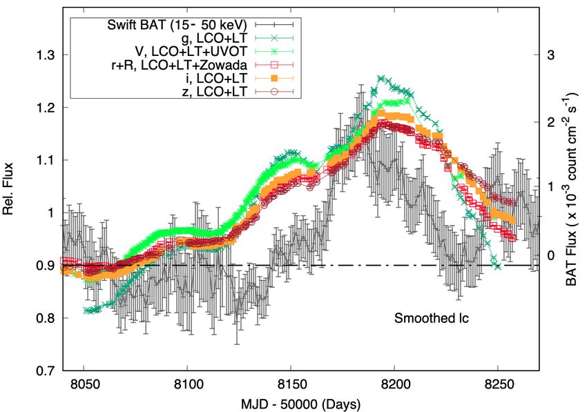
tion of the lightcurve (see Tab 1, Fig. 1 and 2). In order to cover                      the variations observed in the data are present on timescales longer
also the peak of the lightcurve at higher energies we downloaded                         than ≈ a few days, and are not correlated with variations in the
the BAT daily lighcurve from Krimm et al. (2013) from its online                         Crab or other nearby sources. Given also the strong resemblance
archive 3 . BAT lightcurves are known to show spurious variations                        between the BAT and the optical lightcurve, we conclude that the
due to the large field of view used with coded-mask technology.                          observed flare is most probably due to an intrinsic variation of the
Even though the source detection is not significant at a 5 σ level,                      source and not a systematic effect.

                                                                                               Given the low statistics of the data, we applied a 10-day box-
3   https://swift.gsfc.nasa.gov/results/transients/                                      car filter to smooth the lightcurve. In order to be able to compare

MNRAS 000, 1–19 (2021)
8

                                                                                                                                                                                                                                                          Band    Wavelength (Å)   Fvar (%)     peak r      Lag FRRS [days]      peak r      Lag FRRS [days]      peak r       Lag FRRS [days]   Lag Javelin [days]
                                                                                                                                                                                                                                                                                               (Linear)                        (Box-car)                       (un-filtered)

                                                                                                                                                                                                                                                          X-ray        0.25          17.6     0.29 ± 0.05      -0.03+0.53
                                                                                                                                                                                                                                                                                                                    −0.12     0.38± 0.05        0.15+0.37
                                                                                                                                                                                                                                                                                                                                                    −0.17      0.65 ± 0.09        -0.13+0.88
                                                                                                                                                                                                                                                                                                                                                                                       −2.47             -0.17+0.3
                                                                                                                                                                                                                                                                                                                                                                                                              −0.04
                                                                                                                                                                                                                                                                                                                                                                                                                      F. M. Vincentelli et. al

                                                                                                though they are probably due to artifacts.
                                                                                                                                                                                                                                                          UVW2        1928           15.3          -               -               -                -                -                -                           -

                                                                                                                                                                                                                                                          UVM2        2246           13.8     0.88 ± 0.02      -0.14+0.39
                                                                                                                                                                                                                                                                                                                    −0.11     0.77 ± 0.03       0.03+0.15
                                                                                                                                                                                                                                                                                                                                                    −0.13      0.98 ± 0.01        0.56+1.19
                                                                                                                                                                                                                                                                                                                                                                                      −0.56
                                                                                                                                                                                                                                                                                                                                                                                                          0.01+0.03
                                                                                                                                                                                                                                                                                                                                                                                                              −0.01

                                                                                                                                                                                                                                                          UVW1        2600           11.5     0.86 ± 0.02      -0.05+0.25
                                                                                                                                                                                                                                                                                                                    −0.15
                                                                                                                                                                                                                                                                                                                              0.72 ± 0.04       0.04+0.18
                                                                                                                                                                                                                                                                                                                                                    −0.12      0.97 ± 0.01        0.62+1.63
                                                                                                                                                                                                                                                                                                                                                                                      −0.67
                                                                                                                                                                                                                                                                                                                                                                                                          0.01+0.05
                                                                                                                                                                                                                                                                                                                                                                                                              −0.02

                                                                                                                                                                                                                                                          U           3465           10.8     0.72 ± 0.03      -0.01+0.41     0.57 ± 0.04       0.14+0.26      0.95 ± 0.01        0.45+1.10               0.03+0.18

                         to decay with a slower rate as a function of wavelength.
                                                                                                                                                                                                                                                                                                                    −0.29                           −0.24                             −0.85                   −0.16

                                                                                                                                                                                                                                                          B           4392           8.2      0.68 ± 0.04      0.69+0.37
                                                                                                                                                                                                                                                                                                                   −0.33      0.523 ± 0.05      0.66+0.62
                                                                                                                                                                                                                                                                                                                                                    −0.28      0.93 ± 0.01        0.84+1.04
                                                                                                                                                                                                                                                                                                                                                                                      −0.96
                                                                                                                                                                                                                                                                                                                                                                                                          0.31+0.32
                                                                                                                                                                                                                                                                                                                                                                                                              −0.38

                         faster that the one observed at lower energy, the optical bands seem
                         Moreover it is clear that while the rise of the BAT is significantly
                         peak in the 15-50 keV band is seen at approximately MJD 58180.
                         procedure to the ground based ones. As shown in Fig. 5, a clear
                         properly its behaviour with the other filters, we applied the same
                                                                                                                                                                                                                                                          Bz          4500            -       0.68 ± 0.04      0.03+1.02
                                                                                                                                                                                                                                                                                                                   −0.78           -                -          0.93 ± 0.01        0.31+1.34
                                                                                                                                                                                                                                                                                                                                                                                      −1.16
                                                                                                                                                                                                                                                                                                                                                                                                                  -

                                                                                                                                                                                                                                                          Gz          r500            -       0.68 ± 0.04      -0.22+0.97
                                                                                                                                                                                                                                                                                                                    −1.33          -                -          0.93 ± 0.01        -0.71+1.01
                                                                                                                                                                                                                                                                                                                                                                                       −0.59
                                                                                                                                                                                                                                                                                                                                                                                                                  -

                                                                                                                                                                                                                                                          Rz          6500            -       0.55 ± 0.05      0.99+0.76
                                                                                                                                                                                                                                                                                                                   −1.34           -                -          0.94 ± 0.01        1.14+1.36
                                                                                                                                                                                                                                                                                                                                                                                      −1.09                       -

                                                                                                                                                                                                                                                          g           4770           14.1      0.7 ± 0.1       1.04+0.31
                                                                                                                                                                                                                                                                                                                   −0.24      0.42 ± 0.11       1.46+1.04
                                                                                                                                                                                                                                                                                                                                                    −0.56
                                                                                                                                                                                                                                                                                                                                                               0.93 ± 0.03        0.87+1.03
                                                                                                                                                                                                                                                                                                                                                                                      −0.47               1.02+0.07
                                                                                                                                                                                                                                                                                                                                                                                                              −0.09

                                                                                                                                                                                                                                                          V           5468           12.7     0.78 ± 0.03       0.96+0.5
                                                                                                                                                                                                                                                                                                                    −0.4      0.53 ± 0.06       1.75+0.6
                                                                                                                                                                                                                                                                                                                                                    −0.35
                                                                                                                                                                                                                                                                                                                                                               0.97 ± 0.01        2.05+0.85
                                                                                                                                                                                                                                                                                                                                                                                      −0.80               2.16+0.84
                                                                                                                                                                                                                                                                                                                                                                                                              −0.05

                                                                                                                                                                                                                                                          r           6400           9.4      0.55 ± 0.05      1.54+0.51
                                                                                                                                                                                                                                                                                                                   −0.39       0.5 ± 0.05       2.30+0.44
                                                                                                                                                                                                                                                                                                                                                    −0.32      0.94 ± 0.01        2.79+1.27
                                                                                                                                                                                                                                                                                                                                                                                      −1.49               3.04+0.03
                                                                                                                                                                                                                                                                                                                                                                                                              −0.54

                                                                                                                                                                                                                                                          i           7625           10.7     0.54 ± 0.05      1.50+0.75
                                                                                                                                                                                                                                                                                                                   −0.40      0.42 ± 0.05       2.72+0.63
                                                                                                                                                                                                                                                                                                                                                    −0.42      0.91 ± 0.01        2.69+0.86
                                                                                                                                                                                                                                                                                                                                                                                      −0.69
                                                                                                                                                                                                                                                                                                                                                                                                          2.29+0.52
                                                                                                                                                                                                                                                                                                                                                                                                              −0.18

                                                                                                                                                                                                                                                          z           9132           9.4      0.51 ± 0.05      2.40+1.05
                                                                                                                                                                                                                                                                                                                   −0.50
                                                                                                                                                                                                                                                                                                                              0.46 ± 0.06       2.39+0.76
                                                                                                                                                                                                                                                                                                                                                    −0.44      0.91 ± 0.01        2.66+1.74
                                                                                                                                                                                                                                                                                                                                                                                      −0.96
                                                                                                                                                                                                                                                                                                                                                                                                          2.09+0.06
                                                                                                                                                                                                                                                                                                                                                                                                              −0.04

MNRAS 000, 1–19 (2021)
                         tours were derived in the same way as described in the previous
                         lead to any significant differences in our results. Confidence con-
                         days) in the choice of the dates and of the box-car width did not
                         between MJD 58140 and 58240. Sensibly small changes (≈few
                         the correlation between the BAT and the g band, including the data
                              As in the previous section we computed the DCF to quantify
                                                                                                Table 2. Results of the lag vs UVW2 band computed between different bands. For sake of completeness we reported even the lags with multiple peaks, even
Mrk 110 continuum reverberation lags                              9

Table 3. Lag vs g band using the smoothed lightcurves: i.e. after applying a   computed by using the long-term lightcurve. The excesses shown
10 day box-car moving average. Values are plotted in Fig. 5, bottom panels.    around 20 light days in the response of some filters are likely due to
                                                                               the presence of an X-ray dip around MJD 58060. The modelling us-
                           Band      Lag [days]
                                                                               ing the UVW2 filter as a reference band showed a smoother trend.
                                                                               Nevertheless the consistency of the shape of the response function
                           BAT       -9.43 +1.53
                                           −1.27                               among the different filters indicates that the presence of an extra
                           V          0.28+1.57                                component acting at longer timescales.
                                          −0.78
                                                                                    The variable emission from an illuminated accretion disc is
                           r          2.40+0.55
                                          −0.78
                                                                               expected to produce an increasing lag (τ) as a function of wave-
                                                                               length (λ) as follows (Cackett et al. 2007):
                           i          3.94+0.76
                                          −0.59

                                                                                        λ β
                                                                                            !      
                           z         8.01+1.10
                                                                               τ = α 
                                                                                                    
                                         −0.70                                                 − 1                                                    (1)
                                                                                          λ0

section. Although the exact lag is not well defined by this simple                   Where λ0 is the reference band wavelength (UVW2 band in
DCF, the peak is around a lag of about 15 days and is significant at           this case: 1929 Å) and β=4/3 for a Shakura & Sunyaev (1973) ac-
just below the 99 % confidence level.                                          cretion disc. In our dataset we found two different components act-
      In particular, we use the same power spectral parameters                 ing on different timescales. From the values of the lags and from
to synthesise BAT lightcurves as are quoted for the earlier XRT                the shape of the responses obtained by MEMEcho analysis, the
lightcurve. Both BAT and long-term g-band have here been                       short timescale component resembles the behaviour of an illumi-
smoothed, which will remove high frequency variability and should              nated accretion disc. Given this we perform a polynomial fit to the
steepen the power spectrum. The power spectrum for the smoothed                lag-spectrum obtained with the linearly de-trended lightcurve with
BAT lightcurve is reasonably well fitted by a single power law of              Eq. 1 (fixing β=4/3) and obtained α = 0.28 ± 0.04 days with a re-
slope -1.5 but the bend frequency derived by the method of Sum-                duced χ2 of 0.63. The low value is due to the large errors. We also
mons et al. (2008) is within the range of the power spectrum so a              fitted the lag leaving the power law index (β) as a free parameters
model changing slope from -1 at low frequencies to -2.8 at higher              and found α = 0.1 ± 0.06 days and β = 2.1 ± 0.4. The addition of a
frequencies could also be fitted. We have tried a variety of different         free parameter decreases the reduced χ2 (0.44). This is mainly due
underlying BAT power spectral shapes and the peak significance                 to the very short lag measured below 4000 Å. Even though the best
reaches the 99 % confidence level.                                             slope is marginally steeper, the small χ2 and the large errors do not
      We then computed the lags as function of wavelength with                 allow us to determine a significant deviation from the predictions
the FRRS method by using the 10-days smoothed lightcurves, and                 of a standard accretion disc.
choosing the g filter as reference band. The lag probability distri-                 We then performed a more detailed modelling using the same
butions are shown in Fig. 5 (bottom right panel). As expected the              numerical code used by McHardy et al. (2018). This model com-
g is lagging behind the BAT curve by ≈10 days. The lag increases               putes the response function of a Shakura & Sunyaev (1973) ac-
as function of wavelength, going from few days in the V band to                cretion disc illuminated by a “lamp-post" X-ray source (i.e. an
almost 10 days for the g vs z band (see Tab. 3 and Fig. 5, bottom              point-source located over the rotation axis of the disc at a certain
panels). Given the shape of the lightcurves it is clear that the origin        height). The expected lag is taken as half the time for the total light
of the measured delay is the slower response of the longer wave-               to be received. We considered a mass of 2 × 10⁷ M (Bentz &
length during the decay after the peak. However it is interesting to           Katz 2015), an accretion-rate of L/LEdd =40% (Meyer-Hofmeister
notice that the lag spectrum for the long timescales seems to follow           & Meyer 2011), a source height of 6 gravitational radii (RG ), and an
a linear trend from X-ray to near-IR (See Fig. 5). We also tested the          inclination of 45◦4 . As shown in Fig. 4, even though the data points
goodness of the lag by changing the width of the box-car, finding a            at shorter wavelengths seem to present a flatter trend, the predicted
stable lag between 5 and 13 days. For shorter width the statistics be-         lag is in good agreement with the observations.
comes too low to measure a significant lag; for larger box-cars, the
long term trend is distorted by the smoothing, changing the value
of the lag.
                                                                               3.3     Spectral Energy Distribution and Energetics
                                                                               3.3.1    Flux-Flux analysis
3.2   Reverberation Modelling
                                                                               In order to better characterize the origin of the variable emission,
As a first unbiased approach we attempted to model and reproduce               we performed a flux-flux analysis in order to separate the constant
the variable emission from an X-ray corona illuminating the accre-             (galaxy) and variable (AGN) components following Cackett et al.
tion disc through the MEMECHO algorithm (Horne 1994) using
all the collected lightcurves: i.e. attempting to reconstruct the im-
pulse response function of the system through a maximum-entropy                4 An inclination of 40◦ is usually taken as a standard value for this class of
solution method (see also McHardy et al. 2018). We chose the X-
                                                                               sources (Cackett et al. 2007; Fausnaugh et al. 2016; Kammoun et al. 2019,
rays as a reference band. The algorithm manages to reconstruct
                                                                               2021b). Recent X-ray spectral timing measurements of a similar source
the lightcurve at lower energies, with an acceptable chi square                have shown evidence of a higher inclination (Alston et al. 2020, see how-
(χ2 /N = 1.1). The obtained responses show clearly a broadening as             ever Caballero-García et al. 2020). We notice that while the inclination is
a function of wavelength. However, it is also interesting to notice            known to have a strong effect on the X-ray spectrum, the dependence of the
that almost all responses (especially at longer wavelengths) require           optical lags is expected to be negligble (Cackett et al. 2007; Starkey et al.
a long tail which extends to ≈ 10-20 days, as seen also by the lag             2016; Kammoun et al. 2021b).

MNRAS 000, 1–19 (2021)
10           F. M. Vincentelli et. al

                                                                                                 0.07
                     15                                                                                                                      BAT
                                                                                                                                               V
                                                                                                 0.06                                        r+R
                     10                                                                                                                         i
                                                                                                                                               z
                                                                                                 0.05
                      5
       Lag (days)

                                                                                   Frequency

                                                                                                 0.04
                      0
                                                                                                 0.03
                    −5
                                                                                                 0.02
                    −10
                                                                                                 0.01
                                                      Best optical fit
                    −15
                                                                                                    0
                          0   2000   4000      6000        8000          10000
                                                 °                                                   -20   -15   -10    -5        0     5   10      15   20
                                     Wavelength (A)
                                                                                                                             Lag (Days)

Figure 5. Top Panel: Lightcurves used for the long-term trend analysis. Bottom-Left Panel: Lag vs wavelength plot using long timescales. Bottom-Right Panel:
Lag distributions from which the lag spectrum was obtained.

(2020) (see also Cackett et al. 2007; McHardy et al. 2018). We                                 band by extrapolating the best-fitting relations to where the first
fitted the light curves using the following linear model:                                      band crosses fλ = 0. The constant spectrum is consistent with the
                                                                                               past host galaxy measurements by Sakata et al. (2010). The rms
f (λ, t) = Aλ (λ) + Rλ (λ) · X(t)                                            (2)               spectrum follows a λFλ ≈ λ−4/3 , as expected form the predictions
                                                                                               of an accretion disc.
     Where X(t) is a dimensionless light curve with a mean of 0
and standard deviation of 1. Aλ (λ) is a constant for each light curve,                             We then analysed the long-term trend using the ground-based
and Rλ (λ) is the rms spectrum. All three parameters are determined                            data. When plotting the modelled lightcurve with respect to the real
by the fit. Such a simplified model does not take account of any                               observations, only the rise is well reproduced, while of the decay
time lags, adding some scatter around the linear flux-flux relations.                          follows a different trend (see Fig. 8, top panels). We therefore anal-
We first focused using the rise of the lightcurve during which all                             ysed the tail of the long-term variation separately (see Fig. 8, bot-
the facilities were observing. The results of the fit are shown in                             tom panels), finding a significantly steeper spectrum (λFλ ≈ λ−2 ).
Fig. 7. We estimate the minimum host galaxy contribution in each                               The presence of a variable component different from a standard

                                                                                                                                            MNRAS 000, 1–19 (2021)
Mrk 110 continuum reverberation lags                       11
                                                                               ting component it is necessary to take into account the illuminating
                                                                               fraction. Following the assumptions described in the previous sec-
                                                                               tion we estimate that total amount of radiation impacting the disc
                                                                               is 3 × 10⁻¹¹ ergs s−1 cm−2 . Moreover, given that the source can vary
                                                                               up to 1 count s−1 the variable flux we can take as an upper limit to
                                                                               the variable flux ≈ 2 × 10⁻¹¹ ergs s−1 cm−2 .
                                                                                     From the rms-spectrum computed in the previous subsection,
                                                                               we obtained a variable optical-UV flux of 2.5×10⁻¹¹ ergs s−1 cm−2 .
                                                                               We conclude therefore that the X-ray variations contain enough en-
                                                                               ergy to power most of the variability seen in the optical-UV (if they
                                                                               are driven by an illuminated accretion disc). We also notice that if
                                                                               the low energy emission is dominated by the BLR, the solid angle
                                                                               to which it is exposed will be much larger, and the argument will
                                                                               still be valid.
                                                                                     The reported estimate for the ionizing variable flux sets a solid
                                                                               lower limit, which, however, is based on a purely phenomenologi-
                                                                               cal model. In order to have a more realistic value, we also fitted the
                                                                               SED using the physically motivated model optxagnf (Done et al.
                                                                               2012). The model assumes the presence of emission from an ex-
                                                                               tended hot corona, going from the soft X-rays to the far UV, while
                                                                               optical and near UV emission would be dominated by the accretion
                                                                               disc.
                                                                                     We included optical and UV data average fluxes, subtracting
                                                                               the galactic contribution. The fit was performed by fixing mass
                                                                               accretion-rate L/LEdd =40% and spin (a) to 0. Mass, redshift and
                                                                               distance were fixed accordingly to values reported in the introduc-
Figure 6. Results from the MEMEcho modelling. Left Panels: Inferred re-        tion. The best fit model reproduced the data with an acceptable chi
sponse functions to be applied to the X-ray band in order to reconstruct the   square (χ2 / d.o.f = 769 / 594; see Tab. 4). Some excess is found
lightcurves at lower energies. Right panels: Observed (green points) and       at higher energies and in the UVOT band. This means that the flux
modelled lightcurves (blue line).                                              will be slightly overestimated. We also attempted to fit the data with
                                                                               a = 0.998, but, despite values were still in the same range of uncer-
                                                                               tainties of the previous fit, the obtained χ2 was significantly worse
accretion disc can explain the presence of a longer lag at longer              (χ2 /d.o.f.≈2). However an acceptable χ2 was found for a mass of
timescales.                                                                    2.5 ×10⁷ M (which is still within the range of uncertainties for
                                                                               most f-factors Bentz & Katz 2015). We estimated a total ionizing
                                                                               flux (5 eV -1000 keV) of Fion ≈ 6× 10⁻¹⁰ erg cm−2 s−1 (i.e. Lion ≈7×
3.3.2   SED: optical-UV/X-ray broadband                                        1045 erg s−1 ).
The analysis reported so far shows the presence of a clear connec-
tion between the X-ray and optical-UV variability, but does not take
                                                                               3.3.3   HST spectroscopy
into account the energy budget of the two components. In order to
quantify it, we estimated the variable flux in the different bands.            The diffuse continuum emission from the BLR will be a source of
We therefore built the X-ray spectral energy distribution from the             wavelength-dependent lags in addition to lags from reprocessing
XRT data including also the Mrk 110 BAT 70 month catalog spec-                 in the accretion disc (Korista & Goad 2001, 2019; Lawther et al.
trum. The flux in the 14-195 keV range is 5.7 × 10⁻¹¹ ergs cm−2 s−1            2018). In order to estimate the contribution from the BLR diffuse
with a power law slope (Γ) of 2. The XRT data (0.3-10 keV), in-                continuum we obtained Hubble Space Telescope (HST) spectra of
stead, shows a harder slope (Γ3−5keV =1.66± 0.07; see Fig. 9, right            Mkn 110. Observations were performed on 2017-12-25, 2018-01-
panel). This has already been seen in past studies (Idogaki et al.             03, and 2018-01-10 using STIS. Observations were taken with the
2018) and suggests the presence of the so-called “Compton hump"                52” × 0.2” aperture using the G230L, G430L and G750L grat-
(see e.g. Guilbert & Rees 1988; Lightman & White 1988; George                  ings. During each epoch exposures totally 800s (G230L), 180s
& Fabian 1991). We therefore applied a simple model for an expo-               (G430L and 180s (G750L) were obtained. In addition to the stan-
nentially cut-off power law spectrum, reflected by neutral material            dard pipeline-processing we used the stis_cti package to apply
(i.e. pexrav; Magdziarz & Zdziarski 1995). We grouped the XRT                  Charge Transfer Inefficiency corrections to the data. Moreover, we
spectrum with a minimum of 30 counts per bin using the FTOOL                   used the contemporaneously obtained fringe flats to defringe the
grppha. We included in the fit a broad line for Kα and the black-              G750L spectra. Any remaining large outliers in the spectrum that
body emission for the soft excess. The results are reported in Tab.            were identified visually as hot pixels were removed manually.
4 under Model 1. We obtained a fit with χ2 of 439 (375 degrees of                    We fit the mean spectrum with a variety of models to estimate
freedom). The model finds a power law slope of Γ ≈ 1.66 ± 0.02                 a plausible contribution from the BLR diffuse continuum. To model
with a cut off at ≈ 120 keV and reflection fraction of 0.2. In order           the BLR diffuse continuum we use a model calculated by Korista &
to estimate the total ionizing flux, we extrapolated the power-law             Goad (2019) that is tailored for NGC 5548. This assumes a locally-
flux in the 3-5 keV band to the 0.1-150 keV range: we obtained                 optimally emitting cloud model for the BLR, with a fixed cloud
F pl = 1 × 10⁻¹⁰ ergs s−1 cm−2 .                                               hydrogen column density of log NH (cm−2 ) = 23, and a gas density
      In order to quantify the connection with the optical-UV emit-            distribution ranging from log nH (cm−3 ) = 8 − 12 (solid black line

MNRAS 000, 1–19 (2021)
12       F. M. Vincentelli et. al

Figure 7. Flux-flux analysis for the rising section of the lightcurve. Left panels shows the lightcurves, and the model (black line). The parametrisation described
in Eq. 2 represents the data well. Top right panel shows the flux-flux relation between the different bands and the driving lightcurve X(t). Bottom right panel
shows the optical/UV variable spectrum. Purple points on the higher section of the graph represent, minimum, average, and maximum values for each band.
Orange continuous line represents the host galaxy contribution. Blue points show the rms spectrum computed as maximum-minimum, while the black point
represent the actual rms. Red dashed lines show the best fit.

in Fig. 4 of Korista & Goad (2019); see that paper for full details                  uum, we exclude the wavelength ranges 3600 – 4050 Å and 8000 –
of the model calculation). We Doppler-broaden the diffuse contin-                    8700 Å from the fit.
uum model by convolving with a Gaussian with FWHM = 5000                                   We further note that we have not calculated a model specific
km/s (Peterson et al. 1998, 2004), consistent with emission from                     to the line luminosities of Mkn 110, and, while the general shape of
the inner BLR in Mrk 110. The presented diffuse continuum model                      the diffuse continuum spectrum is common to all models, the am-
does not include the unresolved high-order Balmer and Paschen                        plitudes of the Balmer and Paschen jumps do depend somewhat on
emission lines redward of those jumps. In addition to the pile-up of                 model assumptions. For these reasons we view the present spectral
Doppler-broadened higher-order Balmer, Paschen, and other emis-                      fitting process as simply providing a guide and an estimate of the
sion lines (HeI and FeII), there is another effect that may serve to                 BLR diffuse continuum contributions to the spectrum.
smooth the free-bound continuum emission jumps in wavelength                               For the underlying AGN continuum emission we try two dif-
space. The cloudy photoionization model simulations all assume                       ferent models - the first is a simple power-law, the second is a stan-
that the wavelengths of the Balmer and Paschen series limits are                     dard accretion disc model (Shakura & Sunyaev 1973) with the outer
at their low-density values, with these values then corrected for at-                radius set to be equivalent to a temperature of 2000K. This pro-
mospheric refraction. However, due to the likely presence of high                    duces a spectrum following the relation Fλ ∝ λ−7/3 through most
density gases within the BLRs of AGN (e.g., 1012−13 cm−3 ), the                      of the wavelength range, but begins to rollover at the longest wave-
wavelengths of the free-bound jumps are likely shifted to somewhat                   lengths. These two models test the sensitivity of the results to as-
longer wavelengths due to the finite sizes of the emitting hydro-                    sumptions about the accretion disc emission. We include both UV
gen atoms. The contributions of mixtures of continuum emission                       and optical Fe ii templates. In the optical we use the template of
from gas spanning the full range of expected densities within the                    Véron-Cetty et al. (2001), while in the UV we use the model of
BLR will thus smooth out somewhat the abrupt free-bound contin-                      Mejía-Restrepo et al. (2018). This latter model has the advantage
uum jumps in wavelength space. This effect is also currently not                     that it covers a broader wavelength range in the UV than other mod-
included in the model spectral template. As neither of these effects                 els. We investigate Doppler broadening in these Fe ii emission mod-
are included in the spectral template for the BLR diffuse contin-                    els by convolving with a Gaussian, and find best fits for FWHM =
                                                                                     3000 km/s. We fit broad and narrow emissions lines with Gaus-

                                                                                                                                       MNRAS 000, 1–19 (2021)
Mrk 110 continuum reverberation lags                             13

Figure 8. The two blocks show the flux-flux analysis for the whole lightcurve (Top) and only the tail (bottom). Left panels shows the lightcurves, and the
model (black line). An hysteresis is evident while using the whole lightcurve. Top right panels shows the flux-flux relation between the different bands and the
driving lightcurve X(t). Bottom right panels shows the optical/UV variable spectrum. Purple points on the higher section of the graph represents, maximum,
average, and maximum values for each band. Orange continuous line represents the galactic contribution. Blue points show the rms spectrum computed as
maximum-minimum, while the black point represent the actual rms. Red dashed lines show λ fλ ∝ λ−4/3 .

MNRAS 000, 1–19 (2021)
14       F. M. Vincentelli et. al

Table 4. Best fit parameters modelling. Model 1 was applied to the only X-ray data from XRT+BAT and is consists in zphabs × [pexrav+zgauss+zbbody].
Errors are reported with 90% confidence interval contour. In order to obtain the fit we froze the following parameters: nH=1.27 ×10²⁰ [cm−2 ] , z = 0.035; He
abund (elements heavier than He) = 1; Fe abund=1. Model 2 includes also optical and UV wavelength, and was parametrized with using zphabs ×optxagnf.
Mass was fixed to 2×10⁷ M , accretion-rate to 40%, Rout =103 RG , spin a to 0.

                                                     Model 1                                                   Model 2
                                        zphabs × [pexrav+zgauss+zbbody]                                    zphabs ×optxagnf
                 Parameter                                                       Best Fit    Parameter                             Best Fit

                 Γ                                                            1.66±0.02      Γ                                  1.72 ±0.02

                 Ecut [keV]                                                       118+33
                                                                                     −22     a                                            0

                 reflfrac                                                       0.21+0.17
                                                                                    −15
                                                                                             Rcor [RG ]                              70±20

                 normpexrav (×10−3 )                                            5.2± 0.1     kTe [keV]                           0.25±0.08

                 LineE [keV]                                                    6.7 ± 0.1    τ                                        11±2

                 σE [keV]                                                         0.3+0.8
                                                                                     −0.2    fpow                                  0.5 ±0.1

                 normzgauss (×10−5 )                                            4.2± 0.1

                 kT [keV]                                                     0.11±0.05

                 normzbbody (×10−5 )                                           5.62± 0.4

                 χ2 / d.of.                                                    648 / 590     χ2 / d.of.                            900/596

Figure 9. Left Panel: X-ray emission spectrum observed by Swift XRT (black points) and BAT (red points) and modelled with Model 1. Right Panel: Ratio
of the data to a simple power-law model.

sians. For the host dust emission from the torus we include a sin-                ing a scale factor allowing it to best-match the data. Although we
gle temperature blackbody with T=1800K, while this is simplistic                  have not optimized the modelled diffuse continuum spectrum for
(e.g. see Appendix A of Korista & Goad 2019, for a more com-                      the broad emission line spectrum of Mrk 110, we checked that the
plex model), longer wavelength coverage is needed to better con-                  spectral fit’s scaling of the diffuse continuum is in line with the
strain this component. We also include an 11 Gyr old solar metallic-              model predictions for NGC 5548 by Korista & Goad (2001, 2019).
ity stellar population model (Bruzual & Charlot 2003), broadened                  The best-fitting model using an accretion disc is shown in Fig. 10,
to the resolution of STIS G430L and G750L. We use the surface                     and generally does a reasonable job of fitting the overall shape of
brightness profile fit parameters of (Bentz et al. 2009) to scale the             the spectrum from ∼1600 – 10000Å.
galaxy flux to the slit width (0.200 ) and extraction size (0.3600 ) used
for these HST data, finding 6.4×10⁻¹⁷ erg s−1 cm−2 Å−1 at 5100Å.                       We perform synthetic photometry on the best-fitting power-
This is fixed in all the fits.                                                    law and disc models to estimate the fraction of the flux contributed
                                                                                  by each component in each of the Swift and LCO filters, and they
     The diffuse continuum model described above is fitted includ-                are given in Table 5. Note that the significantly higher spatial res-

                                                                                                                                  MNRAS 000, 1–19 (2021)
You can also read