An emerging GHG estimation approach can help cities achieve their climate and sustainability goals
←
→
Page content transcription
If your browser does not render page correctly, please read the page content below
LETTER • OPEN ACCESS

An emerging GHG estimation approach can help cities achieve their
climate and sustainability goals
To cite this article: K L Mueller et al 2021 Environ. Res. Lett. 16 084003

View the article online for updates and enhancements.

                                This content was downloaded from IP address 46.4.80.155 on 16/09/2021 at 21:15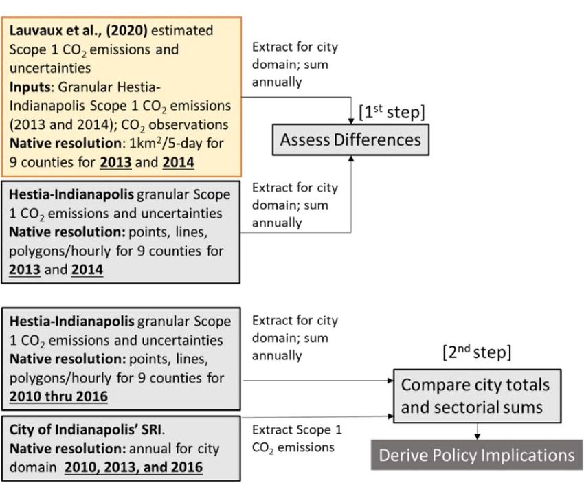
Environ. Res. Lett. 16 (2021) 084003 https://doi.org/10.1088/1748-9326/ac0f25
LETTER
An emerging GHG estimation approach can help cities achieve
OPEN ACCESS
their climate and sustainability goals
RECEIVED
25 March 2021 K L Mueller1,∗, T Lauvaux2, K R Gurney3, G Roest3, S Ghosh4, S M Gourdji1, A Karion1,
REVISED P DeCola5 and J Whetstone1
3 June 2021
1
National Institute of Standards and Technology, Gaithersburg, MD, United States of America
ACCEPTED FOR PUBLICATION 2
28 June 2021 Laboratoire des Sciences du Climat et de l’Environnement, Gif-sur-Yvette Cedex, France
3
School of Informatics, Computing, and Cyber Systems, Northern Arizona University, Flagstaff, AZ, United States of America
PUBLISHED 4
20 July 2021
Center for Research Computing, University of Notre Dame, South Bend, IN, United States of America
5
The University of Maryland, College Park, MD, United States of America
∗
Author to whom any correspondence should be addressed.
Original content from
this work may be used E-mail: Kimberly.Mueller@nist.gov
under the terms of the
Creative Commons Keywords: emissions, cities, approaches, greenhouse gas, carbon accounting, GHG observations, GHG mitigation targets
Attribution 4.0 licence.
Supplementary material for this article is available online
Any further distribution
of this work must
maintain attribution to
the author(s) and the title
of the work, journal Abstract
citation and DOI. A credible assessment of a city’s greenhouse gas (GHG) mitigation policies requires a valid account
of a city’s emissions. However, questions persist as to whether cities’ ‘self-reported inventories’
(SRIs) are accurate, precise, and consistent enough to track progress toward city mitigation goals.
Although useful for broad policy initiatives, city SRIs provide annual snapshots that may have
limited use to city managers looking to develop targeted mitigation policies that overlap with other
issues like equity, air quality, and human health. An emerging approach from the research
community that integrates ‘bottom-up’ hourly, street-level emission data products with ‘top-down’
GHG atmospheric observations have begun to yield production-based (scope 1) GHG estimates
that can track changes in emissions at annual and sub-annual timeframes. The use of this
integrated approach offers a much-needed assessment of SRIs: the atmospheric observations are
tied to international standards and the bottom-up information incorporates multiple overlapping
socio-economic data. The emissions are mapped at fine scales which helps link them to attribute
information (e.g. fuel types) that can further facilitate mitigation actions. Here, we describe this
approach and compare results to the SRI from the City of Indianapolis which shows a yearly
difference of 35% in scope 1 emissions. In the City of Baltimore, we show that granular emission
information can help address multiple issues, e.g. GHG emissions, air pollution, and inequity, at
the sub-zip code scale where many roots and causes for each issue exist. Finally, we show that the
incorporation of atmospheric concentrations within an integrated system provides rapid,
near-real-time feedback on CO2 emissions anomalies that can uncover important behavioral and
economic relationships. An integrated approach to GHG monitoring, reporting and verification
can ensure uniformity, and provide accuracy to city-scale GHG emissions, scalable to states and the
nation—ultimately helping cities meet stated ambitions.
1. Introduction the shortcomings of international climate treaties,
regulation, and climate finance/carbon markets (Seto
Many cities across the globe recognize their impact et al 2014, IPCC 2018). Typical near-term city mit-
on climate change and have committed to long- igation targets range between 30% and 50% reduc-
term, ambitious greenhouse gas (GHG) emission tions by 2030 compared to emissions estimated in a
mitigation targets. The fact that cities are pledging city’s chosen baseline year. More ambitious cities aim
to reduce their GHG emissions suggests that self- to achieve carbon neutrality or be net-zero emitters
organized, city-scale actions might compensate for by 2050 (ARUP, C40 2014).
© 2021 The Author(s). Published by IOP Publishing Ltd
Environ. Res. Lett. 16 (2021) 084003                                                               K L Mueller et al

    A comprehensive accounting, or inventory, of          inventories to support target-setting and mitigation
GHG emissions not only establishes a baseline from        policy. Generally, a city itself accounts for its own
which to prioritize actions but also helps a city mon-    emissions following one of several protocol guidance
itor progress if regularly updated. Although there        documents/tools e.g. ICLEI (2012). Once developed,
are different ways to account for emissions, all          cities can report their self-reported inventory (SRI)
approaches aim to yield estimates that are accurate,      publicly, e.g. through the CDP (formally the Car-
comparable, comprehensive, and complete (Ibrahim          bon Disclosure Project) (https://data.cdp.net/). In
et al 2012, Ramaswami et al 2012). Several guidelines     2017, over 229 cities worldwide reported emissions
have been developed, each having a slightly different     on the CDP (https://data.cdp.net/widgets/kyi6-dk5h,
perspective on how a city should account for their        accessed March 2021) including 45 of the 100 most
emissions (Arioli et al 2020).                            populated cities in the US (Markolf et al 2020).
    The original city-scale guidelines borrowed much           Although mitigation targets set by cities are
from the IPCC framework for nations (IPCC 2006,           impressive, questions have been raised about the
ICLEI 2009). Using this framework, emissions are          accuracy and numerical integrity of reported emis-
estimated by combining activity data with sec-            sions (Satterthwaite 2008, Deetjen et al 2018, Hsu
toral emission factors obtained from, for instance,       et al 2019). This is due, in part, to the city-centric
the IPCC emission factor database (www.ipcc-              nature of the guideline approach. Urban practition-
nggip.iges.or.jp/EFDB/main.php), to provide emis-         ers make multiple subjective decisions based on polit-
sions by economic sector. From this perspective, only     ical, demographic, and socioeconomic circumstances
scope 1 GHG emissions are inventoried (i.e. those         and goals (Kramers et al 2013). They collect and
emissions directly resulting from activities that take    quality control data that may come from different
place within a city’s jurisdiction). For example, elec-   years, national statistics, assumptions, and difficult
tricity generation-related emissions are tied to those    to find sources if local data is not available (Bader
from powerplants that are physically located within a     and Bleischwitz 2009, Hsu et al 2019, Nangini et al
city as opposed to those from any powerplant (inside      2019). Ideally, default emission factors should be
and outside a city) caused by the consumption of          refined (but are not always) to represent local pro-
electricity by city residents (Pichler et al 2017).       cesses (Shan et al 2019). Compiling an SRI takes time,
    Since then, work on corporate supply-chain            resources, and expertise: maintaining consistent up-
(Chen et al 2017) and life-cycle analysis (Ramaswami      to-date inventories is challenging (Nangini et al 2019,
et al 2008, Hillman and Ramaswami 2010, Kennedy           Markolf et al 2020). Many of these logistical and prac-
et al 2010), and trade (Lin et al 2015), provided addi-   tical issues are likely the cause of discrepancies noted
tional perspectives on carbon accounting. These per-      in Gurney et al (2021) rather than fundamental flaws
spectives included inventorying any emissions associ-     within the protocol guidelines themselves.
ated with the consumption of electricity (scope 2) and         It is unclear whether progress can be independ-
emissions associated with the complete supply-chain       ently evaluated since there are no universal stand-
of goods and services (scope 3). A scope 3 approach       ards to chart progress (Markolf et al 2020). Indeed,
allows a city to allocate emissions from factories        the decentralized nature of climate action largely puts
and commercial business worldwide to residents that       the onus on a city itself to independently evaluate
consume products. A ‘consumption-based’ approach          progress. Protocol guidelines recommend that cities
generally involves all three scopes’ emissions, while a   choose the verification that meets their needs and
‘production-based’ perspective considers only scope       capacity (ICLEI 2012) with only a few having the
1 emissions.                                              budget and staff to do so (Blackhurst et al 2011,
    Numerous mixtures and hybrids of consumption-         Markolf et al 2018). Uncertainties associated with
and production-based accounting have been                 SRIs can be >50%, larger than many reduction goals
developed and applied at the city-scale (Ramaswami        (Blackhurst et al 2011). Reporting provides a meas-
and Chavez 2013, Chen et al 2016, Seto et al 2016,        ure of transparency but choices made by practition-
Lombardi et al 2017, Jones et al 2018). For example,      ers may not be documented or publicly accessible
many incorporate full transboundary activities to         (Markolf et al 2020). But, details of SRIs and third-
avoid truncation errors at physical boundaries, e.g.      party scrutiny are critical to developing/monitoring a
for aviation or marine sectors, or ways to avoid          mitigation strategy (Hoornweg et al 2011). The extent
the double counting of emissions (Creutzig et al          to which an SRI is accurate, comparable, compre-
2015). Most recently, some yield spatially disaggreg-     hensive, and complete is largely city dependent. Com-
ated emission information (Gately and Hutyra 2017,        paring one city’s SRI to another’s is extraordinarily
Gurney et al 2019a, Han et al 2020, Gurney et al          difficult.
2020b) or the use there of (Lin et al 2014).                   Recent peer-reviewed literature raises questions
    While the academic literature has presen-             about the accuracy of SRIs (specifically CO2 ) due to
ted differing accounting perspectives, cities and         large differences between reported city emissions and
non-government organizational (NGO) networks              those published by academics. These differences cast
have taken up the practical task of building              doubt on whether cities are reducing their emissions

                                             2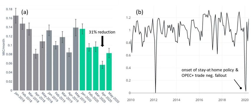
Environ. Res. Lett. 16 (2021) 084003                                                                   K L Mueller et al

as planned or reporting accurate totals. For example,       2019b, Gately and Hutyra 2017). The inversion pro-
Gurney et al (2019a) provides on-road 2010 emis-            cess provides the translation between atmospheric
sions that are 10.7% larger than those reported by the      concentrations and surface emissions (Staufer et al
local metropolitan planning agency in Los Angeles.          2016, Nickless et al 2018, Lauvaux et al 2020, Yadav
Chen et al (2020) reported differences that range           et al 2021); it is in this translation where a fair amount
from −62% to +148% when comparing SRIs to a                 of uncertainty arises at sub-city spatial scales (refer to
downscaled emission product for 12 cities across the        the implication section).
globe. In an analysis of SRIs from 48 U.S. cities,               Here, we present three case studies that brings
Gurney et al (2021) argues that cities under-report         together data from the published literature. This
their scope 1 emissions by 18.3% on average with a          work focuses on scope 1 GHG emissions because
range of −145.5% to 63.5% when compared to a fine-          they (a) can be linked with atmospheric observa-
scale emission product (aka Vulcan). Note, the Vul-         tions (Nangini et al 2019)—the most important
can emission product is consistent with atmospheric         feature, (b) are largely co-located with issues of
radiocarbon (14 ◦ C) measurements at the continental        air quality (Bares et al 2018), environmental justice
scale (Basu et al 2020, Gurney et al 2020a).                (Cushing et al 2018), heat island effects (Chakraborty
     These reported discrepancies suggest that SRIs are     et al 2019), etc, (c) are usually ∼50% of a city’s over-
inconsistent with one another and may contain sys-          all emissions (Kennedy et al 2009), and (d) are more
tematic biases or omissions. The comparisons also           straightforward to estimate (Dodman 2009, Hsu et al
raise numerous questions such as: how well can we           2019) and thus, should be easier to estimate (and
determine whether a city is moving toward meeting           more well-known) than other types of emissions.
its targets? Can we assess whether activities at the city   Thus, any discrepancies in scope 1 estimates between
scale, when aggregated, have a national/global impact       reported emissions (by the city and other groups)
on emissions? Could new perspectives and methods            suggest similar inconsistencies in emissions associ-
help check the accuracy of reported emissions while         ated with other scopes that require more assump-
providing an additional level of consistency?               tions, even more data inconsistencies, etc.
     To this end, the geoscience research com-                   The first case study compares the SRI (scope 1
munity has developed approaches to quantify city            emissions only) for Indianapolis, Indiana with whole-
and regional CO2 and methane (CH4 ) emissions               city emissions estimated with an integrated approach.
(Hutyra et al 2014). These methods integrate ‘top-          We use Baltimore, Maryland in a second case study to
down’ atmospheric GHG observations with granular            show how spatially and temporally explicit emissions
‘bottom-up’ emissions data products using atmo-             can point to specific places where the city can achieve
spheric inversion techniques (Tarantola 2004, Enting        co-benefits. Identifying underlying spatial processes
2018). Atmospheric inversions have a rich history in        not only helps city planners contextualize aggregated
carbon cycling science (Law 1999, Gurney et al 2002,        annual city-wide totals but provides support for tar-
Peters et al 2007, Ogle et al 2015). Their application      geted action. Finally, our third case study, focused on
over the last decade at urban scales have begun to yield    the City of Baltimore, demonstrates that relationships
estimates that can track changes in GHG emissions           between citizen behavior, market forces, and stressors
at annual and sub-annual timeframes (Lauvaux et al          (like weather shocks), are best uncovered using emis-
2016, Sargent et al 2018, Turnbull et al 2019, Yadav        sion information at sub-annual scales. Understand-
et al 2019, Lauvaux et al 2020, Yadav et al 2021).          ing relationships can explain year to year variability
     Each component of the integrated approach, i.e.        in annual emissions and allow cities to concentrate
atmospheric observations, the inversion process, and        on levers to reduce emissions that are within their
the granular data products, brings unique value to          control. Such case studies have not been previously
the estimation of emissions. Atmospheric observa-           presented in the literature, largely because there are
tions are key since they root the granular emis-            only a few applications of an integrated approach at
sion data to an atmospheric measurement of GHG              the urban scale. A summary of SRIs and the integrated
tied to international standards (Tans et al 1990,           approach is provided in table 1.
Tsutsumi et al 2009). Thus, the atmospheric observa-
tions provide a measure of accuracy to the estimates        2. Data and methods
missing from other carbon accounting techniques.
Observations also contain the integral of all sources       In our whole-city case study (figure 1), we extract
in a defined area including anthropogenic emis-             scope 1 CO2 emissions and associated uncertain-
sions and biological fluxes. The granular emissions,        ties from those reported in Lauvaux et al (2020),
whose development has accelerated in the last dec-          for the city of Indianapolis’ jurisdictional boundary
ade, provide detailed information built from multiple       (∼950 km2 ) and sum them annually for 2013 and
data sources, including directly observed emission          2014. Lauvaux et al (2020) employed an integrated
quantities (e.g. from continuous emission monitor-          approach to estimate 1 km2 /5 day emissions for a
ing systems, aka CEMS), providing added specificity         nine county domain for 2013 and 2014 using (a)
(at hourly/building-level scales) (Gurney et al 2012,       high-accuracy atmospheric CO2 observations from

                                               3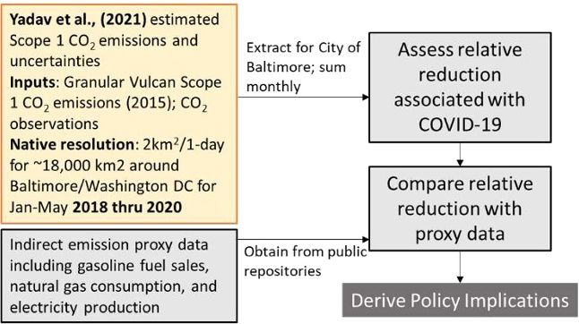
Table 1. Descriptions of SRIs and an integrated approach which includes granular GHG emissions, atmospheric observations, and an inversion link. Symbols, definitions, and references include: (∗ )CO2 equivalents, or CO2 eq,
    allows for the combination of multiple GHG emissions into a single number using global warming potentials (GWPs); (+ ) Hestia, (Gurney et al 2012); (++ ) Vulcan; (Gurney et al 2020b); and (+++ ) ACES, (Gately and Hutyra
    2017); (++++ ) (Michalak et al 2017); (∧ ) observations are available sub-hourly but generally used at the hourly timescale; (∧∧ ) e.g. (Karion et al 2020); (∧∧∧ ) uncertainties from inversion components discussed in the implication
    section, generally much larger than observational uncertainties.

                                                                                                                                                                         Integrated approach
                                                                                                                                                                             Components
    Characteristics                                                 Self reported inventories (SRIs)                          Granular emissions                                         Atmospheric observations/inversion link
                                                                                                                                                                                                                                               Environ. Res. Lett. 16 (2021) 084003

    Units                                                           CO2 eq∗ (mass/year)                                       CO2 and CH4 (mass/time)                                    CO2 and CH4 (mass)
    Spatial scale                                                   Whole city                                                Points/lines/polygons at hourly timescales;                NA
                                                                                                                              Gridded (1 km2 or greater) at various
                                                                                                                              temporal resolutions
    Temporal scale                                                  Annual                                                    Hourly                                                     Hourly∧
    Latency                                                         Periodic updates with multiple yearly gaps                                                                           Real time

4
                                                                                                                              ∼Lags current year
    Input data                                                      Socio-economic data (activity data) and                   Socio-economic data (activity data) and                    Grannular emissions, meteorological-
                                                                    emission factors. Default, nationally,                    emission factors. Nationally, regionally or                dispersion model, assumptions on error
                                                                    regionally, or locally derived. Choices by                locally derived. Consistent across cities.                 characteristics for model components,
                                                                    cities.                                                   Choices by developer.                                      atmospheric observations from in-situ
                                                                                                                                                                                         networks, aircraft, satellite, others. Choices
                                                                                                                                                                                         by developer.
    Reported scope 1                                                Yes (but may not be reported separately                   Yes                                                        NA
                                                                    than scope 2)
                                  Reported production-              Can be hard to isolate total in-boundary                  Yes                                                        —
                                  based total                       scope 1 from scope 2 depending on
                                                                    reporting.
                                  Location specified                No (only whole-city total)                                Yes                                                        —
                                  Reported sectors                  On-road                                                   On-road                                                    —
                                                                    Industrial                                                Industrial                                                 —
                                                                    Residential                                               Residential                                                —
                                                                    Commercial                                                Commercial                                                 —
                                                                    Non-road                                                  Non-road                                                   —
                                                                    Other                                                     Other                                                      —
                                                                                                                              In-domain electrical prod.                                 —
                                                                                                                                                                                                                            (Continued.)
                                                                                                                                                                                                                                               K L Mueller et al
Environ. Res. Lett. 16 (2021) 084003
Table 1. (Continued.)
Integrated approach
Components
Characteristics Self reported inventories (SRIs) Granular emissions Atmospheric observations/inversion link
5
Reported scope 2 Yes (but may not be reported separately Depends if emissions are available outside NA
than scope 1) city boundaries
Location specified No — —
sectors Electricity prod. — —
Reported scope 3 Depends No NA
Location specified No — —
Reported sectors Waste — —
Food — —
Validated City-dependent. No uncertainty Reported whole city uncertainties Uncertainties associated with
reported. observations∧∧ ; uncertainties associated
with inversion link∧∧∧
Reporting CDP, carbonne, others Academic literature, public portals, etc. Academic literature, public portals, etc.
K L Mueller et alEnviron. Res. Lett. 16 (2021) 084003 K L Mueller et al
Figure 1. Flowchart for analysis in the whole-city case study for the City of Indianapolis. The orange box represents the integrated
approach used in Lauvaux et al (2020) to estimate emissions in 2013 and 2014. Since emissions are not available for other years
from the integrated approach, we compare the differences between the extracted and summed emissions from Lauvaux et al
(2020) for the City of Indianapolis and Hestia-Indianapolis (i.e. one component of the integrated system; Gurney et al 2012) for
these 2 years. If the difference is negligible, we plot the extracted and summed Hestia-Indianapolis for 2010 thru 2016; compared
them against the total scope 1 CO2 emissions from the city’s SRI for 2010, 2013, and 2016; and, also compare the sector annual
totals between Hestia-Indianapolis and the city’s scope 1 CO2 emissions in 2013. Note, the City of Indianapolis’ reports scope
1 & 2 CO2 eq. emissions using the Global Protocol for Community-Scale GHG Emission Inventories (GPC); here we extracted the
Scope 1 CO2 emissions for the comparison.
an urban in-situ tower network (figure 3(a)), and (b) an integrated approach. These emissions have been
year-specific scope 1 CO2 Hestia-Indianapolis granu- compared to the City of Baltimore SRI and differ-
lar emissions (1 km2 hr−1 , figure S1 (available online ences were diagnosed by Roest et al (2020). Hestia
at stacks.iop.org/ERL/16/084003/mmedia)) (Gurney on-road emissions are estimated for each road seg-
et al 2012) linked through an inversion. We also sep- ment as detailed in Gurney et al (2020a). Briefly,
arately show Hestia-Indianapolis CO2 emissions and the developers used an inverse distance weighting of
uncertainties (Gurney et al 2012) for the city domain average annual daily traffic (AADT) from the Federal
since they cover a longer timespan (2010–2016). A Highway Administration’s vehicle counting station
summary of the model used in Lauvaux et al (2020), data, which were disaggregated by road type. The
the Hestia-Indianapolis method, means of extract- AADT were then used with the road segment length
ing city emissions and uncertainties, and conversion to estimate the vehicle miles travelled for each road
of CO2 eq to CO2 are provided in the SI along with segment, which provides a relative metric to distrib-
annual totals and sectoral emission sums (table S1). ute county-level FFCO2 emissions from the 2011 EPA
We compare the extracted and aggregated city-wide National Emissions Inventory (NEI). Local gap-filled
emissions from Lauvaux et al (2020) with those of traffic data were used to distribute emissions in time
Hestia-Indianapolis. We derive scope 1 CO2 emission to the hourly scale, though only annual emissions are
from the City of Indianapolis’ Thrive report and GHG used in this study. More details on the on-road emis-
Inventory (2018, 2021) (detailed in table S2). We dir- sion methods can be found in the Vulcan (Gurney
ectly compare the (a) city-wide totals (2010, 2013, et al 2020a) and Hestia-Baltimore (Roest et al 2020).
2016), (b) city reported scope 1 sectoral emissions We also use a housing market typology (HMT) map
(2013) to (c) Hestia-Indianapolis emissions. employed by the city to target interventions and guide
In our sub-city case study, we use the annual municipal investments based on neighborhood con-
sum of the on-road sector CO2 emissions from the ditions (https://planning.baltimorecity.gov/maps-
granular Hestia-Baltimore data product (for the city data/housing-market-typology). Additionally, we
domain only; Roest et al 2020). A city-scale integ- utilize the Environmental Protection Agency’s (EPA)
rated approach cannot be used to estimate emis- National Air Toxic Assessment (2014) (www.epa.gov/
sions for 2014 given atmospheric observation limita- national-air-toxics-assessment) which lists zip-codes
tions for that year. We assume that Hestia-Baltimore where air toxins and emission source types pose res-
provides a realistic spatial representation of on-road piratory health risks for each state. Zip codes used in
emissions that would result from an application of this study were highlighted as having poor air quality
6Environ. Res. Lett. 16 (2021) 084003 K L Mueller et al
difference. This mirrors the results in Lauvaux et al
(2020). Note, that the reported agreement is not
happenstance. Lauvaux et al (2020) biased Hestia-
Indianapolis emissions by up to 10% and achieved
almost identical results at the nine-county scale. The
convergence in estimates demonstrates that high-
accuracy atmospheric CO2 observations within an
integrated system provide the necessary constraint to
adjust granular emissions (if biased) to be consist-
ent with atmospheric CO2 —which accounts for all
Figure 2. Flowchart for analysis for the seasonal/whole-city possible city sectoral CO2 emissions. We do not have
case study for the City of Baltimore. The orange box emissions from the integrated approach for other
represents the integrated approach used in Yadav et al
(2021) to estimate emissions in January–May 2018, 2019,
years. However, we assume the consistency between
and 2020. Emissions were extracted for the City of Hestia-Indianapolis’ city-wide emissions and those
Baltimore jurisdictional domain from the wider estimation extracted/summed from Lauvaux et al (2020) allow us
extent used in Yadav et al (2021). Relative reductions were
estimated and compared to those reported in Yadav et al to confidently use Hestia-Indianapolis’ emissions as
(2021) and evaluated using proxy data. an independent point of comparison to those repor-
ted by the city.
The Hestia-Indianapolis emissions and the city’s
scope 1 reported emissions trend well together for
due primarily to on-road emissions. More informa- each of the three reporting years (figure 3(b)). Note,
tion on data is provided in the SI. this trend does not necessarily reflect reductions
For our seasonal/whole-city case study (figure 2), stemming from the implementation of city-policies
we extract and aggregate monthly scope 1 CO2 emis- but mainly reflects market forces in the electri-
sions and uncertainties for the City of Baltimore city production sector. For example, the Hestia-
(∼240 km2 ) from those reported in Yadav et al (2021). Indianapolis’ electricity sector emissions indicate a
Yadav et al (2021) used an integrated approach, for decrease in emissions from 2014 to 2016 due to fuel
the Baltimore/Washington DC region, to discern the switching at the two largest in-domain power plants
impact of COVID-19 on CO2 emissions. Yadav et al (figure S1), e.g. Harding St. (a 12 unit, 1196 MW
(2021) estimated daily emissions at a native resolu- capacity) and Perry K. (a small steam producing
tion of 2 km2 /daily for these metropolitan regions multi-fired power station). The city’s 2013 and 2016
(∼18 000 km2 for both domains). Emissions were emissions also capture this change.
estimated for January–May 2020 along with coin- However, unlike the trend, the absolute mag-
cident time-periods for 2019 and 2018 (the averages nitudes of both the annual, sectoral totals of Hestia-
providing baseline months). The integrated approach Indianapolis and the city’s SRI are significantly dif-
used high accuracy atmospheric observations from ferent (figure 3(b)). The city’s reported emissions
in-situ tower networks (figure 4(a)) and 2015 gran- are consistently 35% lower for 2010, 2013 and 2016
ular emissions from Vulcan (Gurney et al 2020a). A compared to the Hestia-Indianapolis emissions. Fur-
summary of the method is provided in the SI. To ther analysis suggests that almost all emission sec-
diagnose cause and effect relationships at the whole- tors are underreported in the city’s SRI by different
city scale, we compare features in emission proxy amounts for various reasons (City of Indianapolis
data with the extracted and summed CO2 emis- 2018, tables 2 and S3). The city’s SRI attributes
sion estimates. The emission proxy data includes the majority of GHG emissions to Indianapolis’ in-
natural gas consumption and gasoline data for the domain residential buildings and traffic. But the dif-
State of Maryland from the Energy Information ference in the transportation sector is substantial
Administration (EIA; www.eia.gov/state/?sid=MD); (43%). Given the size of the sector’s emissions, the
(www.eia.gov/dnav/pet/hist). We also use monthly discrepancy questions whether the city will be able
emission data from EPA’s Clean Air Market Database to assess whether it can achieve its goal of reducing
(CAMD; www.epa.gov/airmarkets) for a powerplant on-road emissions by ∼67% in 2025 from a 2016
within the Baltimore city domain. baseline (refer to tables S4 and S5 for policies outlined
in Thrive including public benchmarking).
3. Results and discussions As cities commit to becoming net-zero emitters by
2050, the differences in total emissions will increas-
3.1. Annual/whole-city comparison: Indianapolis ingly be important to reconcile; assessing trends will
After extracting and summing the Lauvaux et al not be enough. As a signatory to the UNFCCC Ini-
(2020) emissions for the City of Indianapolis (as tiative ‘Race to Net Zero’ (https://unfccc.int/climate-
estimated using an integrated approach), we find action/race-to-zero-campaign), the City of Indiana-
them statistically consistent with those from Hestia- polis will have to balance any of its 2050 emissions
Indianapolis for 2013 and 2014, with less than 3% with carbon offsets. Currently, the absolute difference
7Environ. Res. Lett. 16 (2021) 084003 K L Mueller et al
Figure 3. The extent of the wider Indianapolis region defined by the 2016 census, the city’s jurisdictional boundary (black line)
and the locations (black circles) of sites that have CO2 observations. (a) Comparison of Indianapolis’ (1) derived Scope 1 CO2
numbers (green stars) from the city’s SRI, (2) Scope 1 CO2 estimates from Hestia-Indianapolis (black circles), (3) extracted Scope
1 CO2 emissions quantified by Lauvaux et al (2020) (red squares), and (4) a mixture of Scopes 1 and 2 CO2 eq emissions reported
by the City of Indianapolis, (grey diamond). (b) Error bars on (1) and (3) are reported at 2-sigma. Units are reported in million
metric tonnes of CO2 (MMtCO2 ).
Table 2. Summary of Indianapolis Scope 1 CO2 and Hestia-Indianapolis emissions (City of Indianapolis 2018; MMtCO2 /year) per
sector including percent differences.
Reported sectors Indianapolis scope 1 Hestia-Indianapolis Perc. difference Comments
Airport 500 000 174 175 97%
Commercial 650 000 966 541 −39%
Industrial 500 000 785 029 −44%
Onroad/nonroad/railroad 4249 656 6587 072 −43% Less confidence
(largest source)
Residential 1050 000 1130 791 −7% More confid-
ence (second
largest source)
Elec. Prod. (Scope 1) 3919 026 5036 484 −25%
Total 10 868 682 14 680 091 −35%
between Hestia-Indianapolis emissions and the city’s economically disadvantaged communities that are
reported totals is significant (2-sigma) with an aver- disproportionately impacted by air pollution. Note
age annual discrepancy of ∼4 MMTCO2 —raising that at an aggregate city-scale, emissions along inter-
questions as to whether the city will be able to confid- states and arterial roadways make up the largest per-
ently assess their emissions for proper offsetting. For centage of on-road emissions. However, exposure to
example, as an interim step to 2050, the city aims to vehicle exhaust that causes increased respiratory risk
reduce ∼5.86 MMTCO2 by 2025, with 2.2 MMTCO2 are generally associated with proximity to local road-
from the on-road sector (Scope 1) alone. Since ways (Zwack et al 2011). Indeed, for these zip codes,
annual/whole-city emissions estimated from an those streets that contribute 50% or more to over-
integrated approach are consistent with atmospheric all GHG emissions are smaller arterial roads (table 3)
levels of CO2 , they could provide a credible point of which suggests that congestion and ‘street canyons’
comparison to SRIs to ensure proper accounting. may cause significant air pollution levels at these loc-
alities rather than major thoroughfares (Gately 2017).
3.2. Sub-city case study: Baltimore The city aims to use planning activities outlined in
Mitigating GHG emissions can have co-benefits that their CAP (e.g. City of Baltimore, 2014; activity LUT1.
improve quality of life by addressing air pollution and A further outlined in table S7) to decrease trans-
equity issues which occur at the local scale. In the portation related GHG emissions and improve resid-
City of Baltimore, the overlay of zip codes associated ents’ quality of life overall. Figure 4(b) implies that
with very high respiratory risk from transportation information at the zip-code scale may be too coarse
(aka on-road) emissions specified in EPA’s National to effectively achieve such co-benefits, since hotspots
Air Toxic Assessment with Hestia-Baltimore and the and intersections and specific roads within these areas
city’s HMT map enables us to identify neighborhoods are responsible for most emissions and air pollutants.
and roads that have large associated CO2 emissions Beyond achieving co-benefits, sectoral emis-
and air quality criteria pollutants like PM2.5 . As in sions resolved at granular scales can enable city
other studies (Levy et al 2007), figure 4(b) highlights planners detect the largest emitters in the wider
8Environ. Res. Lett. 16 (2021) 084003 K L Mueller et al
Figure 4. The Washington DC/Baltimore region with urban areas defined by the 2016 census, the City of Baltimore (green
polygon) and the locations (black circles) of sites that have CO2 observations are shown in (a). The four zip codes outlined in
(b) are in the 90–100th percentile of those in the State of Maryland with respiratory risk from PM2.5 due to on-road diesel fuel
combustion. They are also within the 85–100th percentile in terms of respiratory risk from all criteria air pollutants (www.epa.gov/
national-air-toxics-assessment). The housing marketplace typology (HMT) map shown in (b) combines sale price, vacancy,
foreclosures, and other variables to indicate stressed areas along with specific streets and their associated Hestia emissions within
these four zip-code. The roads with the most substantial contribution to the zip codes’ total CO2 emissions are shown in table 3.
Table 3. Roadways ranked by their relative contribution to on-road CO2 emissions within each zip code shown in figure 4.
Zip code → 21205 21213 21217 21223
Rank ↓ Name Percent Name Percent Name Percent Name Percent
1 Harbor 41.0 Belair Rd 23.1 I- 83 47.0 US Hwy Route 40 20.8
Tunnel
Throughway
2 US Hwy 40 24.0 State Hwy 151 13.5 US Hwy 1 17.2 W Franklin St 19.9
3 State Hwy 22.8 Harford Rd 13.0 State Hwy 129 8.2 US Hwy 40 13.5
151
4 E Monument 0.9 E North Ave 12.8 Druid Hill Ave 5.3 US Hwy 1 11.7
St
5 E Madison St 0.6 Edison Hwy 0.9 N Monroe St 3.6 Frederick Ave 7.9
6 Ashland Ave 0.6 E Federal St 0.8 Reisterstown Rd 2.0 N Monroe St 3.0
7 E Eager St 0.5 Sinclair Ln 0.8 State Hwy 26 1.5 S Monroe St 2.6
8 McElderry St 0.4 E Biddle St 0.7 W North Ave 1.1 S Fulton Ave 2.5
9 Jefferson St 0.3 Erdman Ave 0.7 W Lafayette Ave 0.3 W Baltimore St 0.6
10 Wright Ave 0.3 N Broadway 0.6 Eutaw Pl 0.3 Edmondson Ave 0.5
urban extent—helping cities achieve their climate (e.g. weather events, sudden shifts in behavior, and
goals. Within its CAP, the city has targeted improv- abrupt market forces) that might be obscured in
ing the energy efficiency of buildings. The city intends annual totals (Perugini et al 2021). However, estim-
to audit commercial and industrial buildings over ates often have latency that lags real-time by 3–5 years
10 000 sqft to identify simple and low-cost energy (figure S2). This may change in the future as more
efficiency measures (City of Baltimore, 2014; activity city-specific data becomes available without too
ESS.1.C). This amounts to ∼3800 buildings with 76% much delay that can be ingested in granular emis-
being commercial (according to Hestia-Baltimore). sion products. In contrast, atmospheric observations
Roest et al (2020) implied that a large fraction of are available near real-time (figure S2). When using
commercial building emissions (∼76%) are from a an integrated approach, the atmospheric observa-
small number of structures. Hestia-Baltimore could tions use ‘older’ granular emissions (for spatial and
help the city prioritize which buildings should be temporal patterns) but ‘pull’ emissions to capture
audited first based on their emissions profiles (table abnormal events for more recent years (Yadav et al
S7). In doing so, Hestia-Baltimore may also be able 2019, Turner et al 2020). Note, the specificity of
to provide a more realistic GHG reduction estim- granular information within an integrated approach,
ate based on efficiency measures implemented at even for a prior year, is important to achieve city-
these structures compared to the reduction numbers totals consistent with atmospheric CO2 (Oda et al
provided in Baltimore’s CAP. 2017).
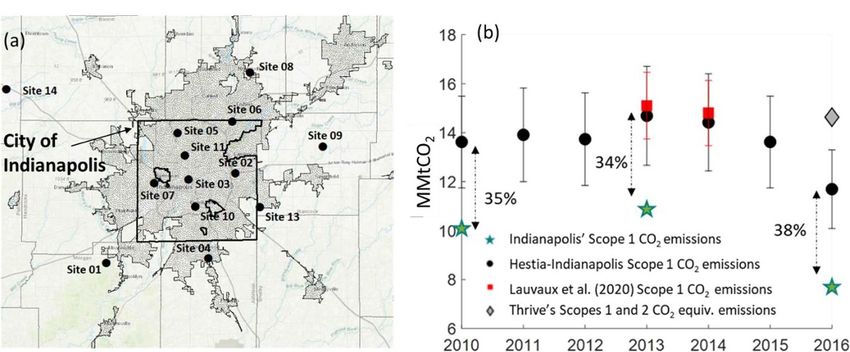
We show this with our extracted Yadav et al (2021)
3.3. Seasonal analysis/whole-city analysis: emissions and associative uncertainties for the City
Baltimore of Baltimore. Our extracted monthly summed CO2
Sub-annual emission information can provide emissions show nearly identical relative reductions
valuable insights into the causes of emissions changes (31% in April 2020; figure 5(a)) in Baltimore as Yadav
9Environ. Res. Lett. 16 (2021) 084003 K L Mueller et al
Figure 5. Extracted monthly mean CO2 emission estimates and uncertainties for January–May 2018, 2019, and 2020 from Yadav
et al (2020) for the City of Baltimore (a). The black arrow points to the 31% relative reduction of CO2 emissions for April 2020
compared to the baseline months of April 2018 and 2019. Error bars represent the 95% confidence intervals (a). Wheelabrator
emissions (www.eia.gov/electricity/data/browser/) are shown in (b).
et al (2021) (33%) but with much wider uncertainty 4. Implications
bounds (1-sigma 30% compared to 11% respect-
ively). These large uncertainties reflect, in part, that Cities have emerged as vanguards of climate
some high-accuracy observations in the city were not leadership and have a stronger relationship with their
available during the height of the change in emissions citizens. But they have a limited set of policy levers
(April 2020). to alter their emissions alone. Coordination and con-
For the City of Baltimore, variations in emission sistency with state, regional, and national emissions is
proxy data (e.g. gasoline fuel sales and natural gas crucial; e.g. cities like Baltimore are counting on state
consumption) explain much (but not all) of the rel- and national measures to help cut their emissions
ative drop in emissions during this time, particu- (20% from the state’s renewable portfolio in 2022,
larly gasoline fuel sales (figure S3). These relation- and 11% from EPA’s passenger vehicle and light duty
ships are explored in Yadav et al (2021). Herein, fuel efficiency standards) but little coordination is
we look at electricity output since, at the national evident. If estimated for a large enough area, emis-
scale, emissions from this sector have been shown sions from an integrated approach are completely
to correlate with pandemic shifts (−15.1% April– consistent across metropolitan, state, regional, and
May relative decline; Gurney et al 2021) when com- national domains while being tied to atmospheric
pared to emission baseline years. There are sev- observations whose accuracy is ensured by interna-
eral powerplants within the city’s boundary. The tional standards. Nested national to regional systems
large Wheelabrator waste-to-energy facility (par- could (a) use various levels of data more quickly,
tially fueled by petroleum waste products) exper- (b) enable policy levers at different scales of gov-
ienced a steep decline in February/March 2020 ernment, (c) foster private-public relationships, (d)
(figure 5(b)). Global petroleum coke (petcoke) sup- avoid truncation issues associated with transporta-
ply was affected by OPEC+ negotiation fallout and tion (e.g. on-road, aviation, and commercial marine
events associated with COVID-19 (Deloitte 2020) shipping), and (e) allow for an assessment of the pro-
which likely explains this jump. The sudden drop gress of action across the county. In this manner, they
in Wheelabrator emissions may have contributed complement existing tools/methods.
to the 30% relative reduction in the Baltimore To provide the type of emission data shown
emissions. herein, continued progress is needed. This involves
The density of people and activities in cities grappling with observational constraints (e.g. in-situ,
make their citizens, economies, and carbon emissions flask, low-cost, and aircraft GHG measurements,
vulnerable to various stressors—both natural and along with satellite retrievals), improving latency
man-made. Understanding the relationships between issues, enhancing workforce capabilities, tackling
CO2 emissions and shocks can help cities (a) design costs, and engaging stakeholders. Presently, imple-
policies to adapt to unexpected events while mitigat- mentation is prohibitively expensive for most city
ing emissions and (b) tease apart those emissions that governments. Organizations like the World Met-
can be influenced by polies (e.g. building codes) com- eorological Organization’s Integrated Global GHG
pared to others outside of the city’s control (e.g. mar- Information System initiative (WMO-IG3 IS; https://
ket forces). ig3is.wmo.int/en/welcome), NGOs, documentary
10Environ. Res. Lett. 16 (2021) 084003 K L Mueller et al
standards organizations, etc must also help. These program Make Our Planet Great Again
organizations can develop a scientifically-based and (CIUDAD). The opinions/recommendations/
internationally recognized framework that would findings/conclusions expressed do not necessarily
ensure that methods are tied to verifiable standards. reflect the views/policies of NIST/US Government.
Researchers are also actively improving elements
of the inversion process that lead to a fair amount ORCID iDs
of uncertainty on estimated emissions. These include:
improving transport models which link observations K L Mueller https://orcid.org/0000-0002-3516-
to emissions in specific locations (Deng et al 2017), 2259
separating atmospheric CO2 entering a city’s domain T Lauvaux https://orcid.org/0000-0002-7697-
(Karion et al 2021), distinguishing anthropogenic 742X
sources from biogenic fluxes (Miller et al 2020), and K R Gurney https://orcid.org/0000-0001-9218-
expanding the suite of measurements to constrain 7164
specific sectors (Nathan et al 2018), etc. Confidently G Roest https://orcid.org/0000-0002-6971-4613
estimating biological contributions using the obser- S Ghosh https://orcid.org/0000-0001-6183-5384
vations could also help with accounting for programs S M Gourdji https://orcid.org/0000-0002-0309-
like composting, increasing green areas, etc.—but 9187
more work is needed to do so. A Karion https://orcid.org/0000-0002-6304-3513
J Whetstone https://orcid.org/0000-0002-5139-
5. Conclusions 9176
In this paper, we show that combining atmo-
spheric GHG observations with granular emissions References
data products in an integrated approach could help
assess the uncertainty of SRIs, support city climate Arioli M S, D’Agosto M D A, Amaral F G and Cybis H B B 2020
The evolution of city-scale GHG emissions inventory
and sustainability goals, and uncover relationships methods: a systematic review Environ. Impact. Assess. Rev.
between GHG emissions and their drivers. Near real- 80 106316
time feedback offers the potential for the ‘course- ARUP, C40 2014 Global Aggregation of City Climate Commitments
correction’ of policies if needed. Methodological Review
Bader N and Bleischwitz R 2009 Measuring urban greenhouse gas
The United Nations Environment Programme emissions: the challenge of comparability Sapiens 2 7–21
(UNEP) estimates that the world would need to cut Bares R et al 2018 The wintertime covariation of CO2 and criteria
carbon emissions by 7.6% per year for the next decade pollutants in an urban valley of the Western United States
to prevent the globe from warming more than 1.5 ◦ C J. Geophys. Res. Atmos. 123 2684–703
Basu S, Lehman S J, Miller J B, Andrews A E, Sweeney C,
above pre-industrial levels (UNEP 2020). To do so, Gurney K R, Xu X, Southon J and Tans P P 2020 Estimating
most cities must achieve net-zero emissions by mid- US fossil fuel CO2 emissions from measurements of
century. But without atmospherically checked emis- (14)C in atmospheric CO2 Proc. Natl Acad. Sci. USA
sion data that speaks to scales of human behavior, 117 13300–307
Blackhurst M, Scott Matthews H, Sharrard A L, Hendrickson C T
this will be difficult. The discrepancies between SRI and Azevedo I L 2011 Preparing US community greenhouse
and our emission estimates shown herein are too large gas inventories for climate action plans Environ. Res. Lett.
to have assurance in reported emissions. Methods 6 034003
like the integrated approach, as demonstrated within Chakraborty T, Hsu A, Manya D and Sheriff G 2019
Disproportionately higher exposure to urban heat in
this work, can help cities achieve multiple goals and lower-income neighborhoods: a multi-city perspective
point global climate efforts in a new and more effect- Environ. Res. Lett. 14 105003
ive direction—all of which are needed to drive down Chen G, Hadjikakou M and Wiedmann T 2017 Urban carbon
emissions locally and globally. transformations: unravelling spatial and inter-sectoral
linkages for key city industries based on multi-region
input–output analysis J. Clean. Prod. 163 224–40
Data availability statement Chen G, Wiedmann T, Hadjikakou M and Rowley H 2016 City
carbon footprint networks Energies 9 602
All data that support the findings of this study are Chen J, Zhao F, Zeng N and Oda T 2020 Comparing a global
included within the article (and any supplementary high-resolution downscaled fossil fuel CO2 emission dataset
to local inventory-based estimates over 14 global cities
files). Carbon Balance Manage. 15 1–15
City of Indianapolis 2018 City of Indianapolis and Marion County,
Indianapolis Greenhouse Gas Emission Inventory Report for
Acknowledgments 2010, 2013, and 2016 vol FY10−11
City of Indianapolis 2021 Thrive Indianapolis
Support for K Gurney, S Ghosh, G Roest, Creutzig F, Baiocchi G, Bierkandt R, Pichler P-P and Seto K C
and P DeCola was provided by NIST 2015 Global typology of urban energy use and potentials for
an urbanization mitigation wedge Proc. Natl Acad. Sci. USA
grants 70NANB10H245, 70NANB19H132,
112 6283–8
70NANB19H129, and 70NANB19H131 respect- Cushing L, Blaustein-Rejto D, Wander M, Pastor M, Sadd J, Zhu A
ively. T Lauvaux was supported by the French and Morello-Frosch R 2018 Carbon trading, co-pollutants,
11Environ. Res. Lett. 16 (2021) 084003 K L Mueller et al
and environmental equity: evidence from California’s ICLEI 2009 International local government GHG emissions
cap-and-trade program (2011–2015) PLoS Med. analysis protocol (IEAP), version 1.0 p 56
15 e1002604 ICLEI 2012 Local Governments for Sustainability USA. U.S.
Deetjen T A, Conger J P, Leibowicz B D and Webber M E 2018 Community Protocol for Accounting and Reporting of
Review of climate action plans in 29 major U.S. cities: Greenhouse Gas Emissions pp 1–67
comparing current policies to research recommendations IPCC 2006 IPCC Guideline for National Greenhouse Gas
Sustain. Cities Soc. 41 711–27 Inventories (Kanagawa: IGES)
Deloitte 2020 Impact of COVID-19 on O&G industry IPCC 2018 Global Research and Action Agenda on Cities and
Deng A et al 2017 Toward reduced transport errors in a high Climate Change Science
resolution urban CO2 inversion system Elementa-Sci. Jones C M, Wheeler S M and Kammen D M 2018 Carbon
Anthrop. 5 20 footprint planning: quantifying local and state mitigation
Dodman D 2009 Blaming cities for climate change? An analysis of opportunities for 700 California cities Urban Plan. 3 35–51
urban greenhouse gas emissions inventories Environ. Urban. Karion A, Callahan W, Stock M, Prinzivalli S, Verhulst K R, Kim J,
21 185–201 Salameh P K, Lopez-Coto I and Whetstone J 2020
Enting I 2018 Estimation and inversion across the spectrum of Greenhouse gas observations from the Northeast Corridor
carbon cycle modeling AIMS Geosci. 4 126–43 tower network Earth Syst. Sci. Data 12 699–717
Gately C K and Hutyra L R 2017 Large uncertainties in Karion A, Lopez-Coto I, Gourdji S M, Mueller K, Ghosh S,
urban-scale carbon emissions J. Geophys. Res. Atmos. Callahan W, Stock M, DiGangi E, Prinzivalli S and
122 11242–60 Whetstone J 2021 Background conditions for an urban
Gately C K, Hutyra L R, Peterson S and Sue Wing I 2017 Urban greenhouse gas network in the Washington, DC, and
emissions hotspots: Quantifying vehicle congestion and air Baltimore metropolitan region Atmos. Chem. Phys.
pollution using mobile phone GPS data Environmental 21 6257–73
Pollution 229 496–504 Kennedy C A, Steinberger J, Gasson B, Hansen Y, Hillman T,
Gurney K R et al 2002 Towards robust regional estimates of CO2 Havránek M, Pataki D, Phdungsilp A, Ramaswami A and
sources and sinks using atmospheric transport models Mendez G V 2009 Greenhouse gas emissions from global
Nature 415 626–30 cities Environ. Sci. Technol. 43 7297–302
Gurney K R et al 2019a Comparison of global downscaled versus Kennedy C, Steinberger J, Gasson B, Hansen Y, Hillman T,
bottom-up fossil fuel CO2 emissions at the urban scale in Havránek M, Pataki D, Phdungsilp A, Ramaswami A and
four U.S. urban areas J. Geophys. Res. Atmos. 124 2823–40 Mendez G V 2010 Methodology for inventorying
Gurney K R et al 2020a The Vulcan version 3.0 high-resolution greenhouse gas emissions from global cities Energy Policy
fossil fuel CO2 emissions for the United States J. Geophys. 38 4828–37
Res. Atmos. 125 e2020JD032974 Kramers A, Wangel J, Johansson S, Höjer M, Finnveden G and
Gurney K R, Liang J, Roest G, Song Y, Mueller K and Lauvaux T Brandt N 2013 Towards a comprehensive system of
2021 Under-reporting of greenhouse gas emissions in U.S. methodological considerations for cities’ climate targets
cities Nat. Commun. 12 553 Energy Policy 62 1276–87
Gurney K R, Mirtra B, Roest G, Dass P, Song Y and Moiz T 2021 Lauvaux T et al 2016 High-resolution atmospheric inversion of
Impact and rebound of near real-time United States fossil urban CO2 emissions during the dormant season of the
fuel carbon dioxide emissions from COVID-19 and large Indianapolis flux experiment (INFLUX) J. Geophys. Res.
differences with global estimates (https://doi.org/ 121 5213–36
10.31223/X5GC9Z) Lauvaux T et al 2020 Policy-relevant assessment of urban CO2
Gurney K R, Patarasuk R, Liang J, Song Y, O’Keeffe D, Rao P, emissions Environ. Sci. Technol. 54 10237–45
Whetstone J R, Duren R M, Eldering A and Miller C 2019b Law R M 1999 CO2 sources from a mass-balance inversion:
The Hestia fossil fuel CO2 emissions data product for the sensitivity to the surface constraint Tellus B 51 254–65
Los Angeles megacity (Hestia-LA) Earth Syst. Sci. Data Levy J I, Wilson A M and Zwack L M 2007 Quantifying the
11 1309–35 efficiency and equity implications of power plant air
Gurney K R, Razlivanov I, Song Y, Zhou Y, Benes B and pollution control strategies in the United States Environ.
Abdul-Massih M 2012 Quantification of fossil fuel CO2 Health Perspect. 115 743–50
emissions on the building/street scale for a large U.S. city Lin J, Hu Y, Cui S, Kang J and Ramaswami A 2015 Tracking urban
Environ. Sci. Technol. 46 12194–202 carbon footprints from production and consumption
Gurney K R, Song Y, Liang J and Roest G 2020b Toward accurate, perspectives Environ. Res. Lett. 10 054001
policy-relevant fossil fuel CO2 emission landscapes Environ. Lin J, Pan D, Davis S J, Zhang Q, He K, Wang C, Streets D G,
Sci. Technol. 54 9896–907 Wuebbles D J and Guan D 2014 China’s international trade
Han P et al 2020 A city-level comparison of fossil-fuel and and air pollution in the United States Proc. Natl Acad. Sci.
industry processes-induced CO2 emissions over the USA 111 1736–41
Beijing-Tianjin-Hebei region from eight emission Lombardi M, Laiola E, Tricase C and Rana R 2017 Assessing the
inventories Carbon Balance Manage. 15 25 urban carbon footprint: an overview Environ. Impact. Assess.
Hillman T and Ramaswami A 2010 Greenhouse gas emission Rev. 66 43–52
footprints and energy use benchmarks for eight U.S. cities Markolf S A, Azevedo I M L, Muro M and Victor D G 2020 Pledges
Environ. Sci. Technol. 44 1902–10 and progress: steps toward greenhouse gas emissions reductions
Hoornweg D, Sugar L and Trejos Gómez C L 2011 Cities and in the 100 largest cities across the United States Brookings
greenhouse gas emissions: moving forward Environ. Urban. Markolf S A, Matthews H S, Azevedo I M L and Hendrickson C
23 207–27 2018 The implications of scope and boundary choice on the
Hsu A et al 2019 A research roadmap for quantifying non-state establishment and success of metropolitan greenhouse gas
and subnational climate mitigation action Nat. Clim. reduction targets in the United States Environ. Res. Lett.
Change 9 11–17 13 124015
Hutyra L R, Duren R, Gurney K R, Grimm N, Kort E A, Larson E Michalak A M, Randazzo N A and Chevallier F 2017 Diagnostic
and Shrestha G 2014 Urbanization and the carbon cycle: methods for atmospheric inversions of long-lived
current capabilities and research outlook from the natural greenhouse gases Atmos. Chem. Phys. 17 7405–21
sciences perspective Earths Future 2 473–95 Miller J B, Lehman S J, Verhulst K R, Miller C E, Duren R M,
Ibrahim N, Sugar L, Hoornweg D and Kennedy C 2012 Yadav V, Newman S and Sloop C D 2020 Large and
Greenhouse gas emissions from cities: comparison of seasonally varying biospheric CO2 fluxes in the Los Angeles
international inventory frameworks Local Environ. megacity revealed by atmospheric radiocarbon Proc. Natl
17 223–41 Acad. Sci. USA 117 26681–7
12Environ. Res. Lett. 16 (2021) 084003 K L Mueller et al
Nangini C, Peregon A, Ciais P, Weddige U, Vogel F and Wang J Satterthwaite D 2008 Cities’ contribution to global warming:
et al 2019 A global dataset of CO2 emissions and ancillary notes on the allocation of greenhouse gas emissions Environ.
data related to emissions for 343 cities Sci. Data 6 180280 Urban. 20 539–49
Nathan B J, Lauvaux T, Turnbull J and Gurney K 2018 Seto K C, Davis S J, Mitchell R B, Stokes E C, Unruh G and
Investigations into the use of multi-species measurements Ürge-Vorsatz D 2016 Carbon lock-in: types, causes, and
for source apportionment of the Indianapolis fossil fuel CO2 policy implications Annu. Rev. Environ. Resour. 41 425–52
signal Elementa-Sci. Anthrop. 6 21 Seto K et al 2014 Human settlements, infrastructure and spatial
Nickless A, Rayner P J, Engelbrecht F, Brunke E-G, Erni B and planning Climate Change 2014: Mitigation of Climate
Scholes R J 2018 Estimates of CO2 fluxes over the city of Change Contribution of Working Group III to the Fifth
Cape Town, South Africa, through Bayesian inverse Assessment Report of the Intergovernmental Panel on Climate
modelling Atmos. Chem. Phys. 18 4765–801 Change (Cambridge: Cambridge University Press)
Oda T, Lauvaux T, Dengsheng L, Rao P, Miles N and Richardson S Shan Y, Liu J, Liu Z, Shao S and Guan D 2019 An
et al 2017 On the impact of granularity of space-based emissions-socioeconomic inventory of Chinese cities Sci.
urban CO2 emissions in urban atmospheric inversions: a Data 6 190027
case study for Indianapolis, IN Elementa-Sci. Anthrop. 5 28 Staufer J et al 2016 The first 1-year-long estimate of the Paris
Ogle S M, Davis K, Lauvaux T, Schuh A, Cooley D and West T O region fossil fuel CO2 emissions based on atmospheric
et al 2015 An approach for verifying biogenic greenhouse inversion Atmos. Chem. Phys. 16 14703–26
gas emissions inventories with atmospheric CO2 Tans P, Fung I Y and Takahashi T 1990 Observational constraints
concentration data Environ. Res. Lett. 10 034012 on the global atmospheric CO2 budget Science
Perugini L, Pellis G, Grassi G, Ciais P, Dolman H, House J I, 247 1431–8
Peters G P, Smith P, Günther D and Peylin P 2021 Emerging Tarantola A 2004 Inverse Problem Theory and Methods for Model
reporting and verification needs under the Paris Agreement: Parameter Estimation (Amsterdam: Elsevier) (https://doi.
how can the research community effectively contribute? org/10.1137/1.9780898717921)
Environ. Sci. Policy 122 116–26 Tsutsumi Y et al 2009 Technical report of global analysis method
Peters W, Jacobson A R, Sweeny C, Andrews A E and Conway T J for major greenhouse gases by the world data center for
et al 2007 An atmospheric perspective on North American greenhouse gases World Meteorological Organization Global
carbon dioxide exchange: carbonTracker Proc. Natl Acad. Atmospheric Watch p 31
Sci. 104 18925–30 Turnbull J C, Karion A, Davis K J, Lauvaux T, Miles N L and
Pichler P-P, Zwickel T, Chavez A, Kretschmer T, Seddon J and Richardson S J et al 2019 Synthesis of urban CO2 emission
Weisz H 2017 Reducing urban greenhouse gas footprints Sci. estimates from multiple methods from the Indianapolis flux
Rep. 7 14659 project (INFLUX) Environ. Sci. Technol. 53 287–95
Ramaswami A and Chavez A 2013 What metrics best reflect the Turner A J, Kim J, Fitzmaurice H, Newman C, Worthington K and
energy and carbon intensity of cities? Insights from theory Chan K et al 2020 Observed impacts of COVID-19 on urban
and modeling of 20 US cities Environ. Res. Lett. 8 035011 CO2 emissions Geophys. Res. Lett. 47 e2020GL090037
Ramaswami A, Chavez A and Chertow M 2012 Carbon UNEP 2020 Emissions Gap Report 2020—Executive Summary
footprinting of cities and implications for analysis of urban (Nairobi)
material and energy flows J. Ind. Ecol. 16 783–5 Yadav V, Duren R, Mueller K, Verhulst K R, Nehrkorn T and Kim J
Ramaswami A, Hillman T, Janson B, Reiner M and Thomas G et al 2019 Spatio-temporally resolved methane fluxes from
2008 A demand-centered, hybrid life-cycle methodology for the Los Angeles megacity J. Geophys. Res. Atmos.
city-scale greenhouse gas inventories Environ. Sci. Technol. 124 5131–148
42 6455–61 Yadav V, Ghosh S, Mueller K, Karion A, Roest G and Gourdji S
Roest G S, Gurney K R, Miller S M and Liang J 2020 Informing et al 2021 The impact of COVID-19 on CO2 emissions in
urban climate planning with high resolution data: the Hestia the Los Angeles and Washington DC/Baltimore
fossil fuel CO2 emissions for Baltimore, Maryland Carbon metropolitan areas Geophys. Res. Lett. 48 e2021GL092744
Balance Manage. 15 22 Zwack L M, Paciorek C J, Spengler J D and Levy J I 2011
Sargent M et al 2018 Anthropogenic and biogenic CO2 fluxes in Characterizing local traffic contributions to particulate air
the Boston urban region Proc. Natl Acad. Sci. USA pollution in street canyons using mobile monitoring
115 7491–6 techniques Atmos. Environ. 45 2507–14
13You can also read