Effects of metallic system components on marine electromagnetic loop data - OceanRep
←
→
Page content transcription
If your browser does not render page correctly, please read the page content below
Geophysical Prospecting, 2020, 68, 2254–2270                                                                 doi: 10.1111/1365-2478.12984

Effects of metallic system components on marine electromagnetic loop
data
Konstantin Reeck1∗ , Hendrik Müller2 , Sebastian Hölz1 , Amir Haroon1 ,
Katrin Schwalenberg2 and Marion Jegen1
1 GEOMAR    Helmholtz Centre for Ocean Research Kiel, Wischhofstr. 1-3, Kiel, 24148, Germany, and 2 BGR – Federal Institute for
Geosciences and Natural Resources Germany, Stilleweg 2, Hannover, 30655, Germany

Received December 2019, revision accepted May 2020

                                              ABSTRACT
                                              Electromagnetic loop systems rely on the use of non-conductive materials near the
                                              sensor to minimize bias effects superimposed on measured data. For marine sensors,
                                              rigidity, compactness and ease of platform handling are essential. Thus, commonly
                                              a compromise between rigid, cost-effective and non-conductive materials (e.g. stain-
                                              less steel versus fibreglass composites) needs to be found. For systems dedicated to
                                              controlled-source electromagnetic measurements, a spatial separation between critical
                                              system components and sensors may be feasible, whereas compact multi-sensor plat-
                                              forms, remotely operated vehicles and autonomous unmanned vehicles require the use
                                              of electrically conductive components near the sensor. While data analysis and geolog-
                                              ical interpretations benefit vastly from each added instrument and multidisciplinary
                                              approaches, this introduces a systematic and platform-immanent bias in the measured
                                              electromagnetic data. In this scope, we present two comparable case studies target-
                                              ing loop-source electromagnetic applications in both time and frequency domains: the
                                              time-domain system trades the compact design for a clear separation of 15 m between
                                              an upper fibreglass frame, holding most critical titanium system components, and a
                                              lower frame with its coil and receivers. In case of the frequency-domain profiler, the
                                              compact and rigid design is achieved by a circular fibreglass platform, carrying the
                                              transmitting and receiving coils, as well as several titanium housings and instruments.
                                              In this study, we analyse and quantify the quasi-static influence of conductive objects
                                              on time- and frequency-domain coil systems by applying an analytically and experi-
                                              mentally verified 3D finite element model. Moreover, we present calibration and op-
                                              timization procedures to minimize bias inherent in the measured data. The numerical
                                              experiments do not only show the significance of the bias on the inversion results, but
                                              also the efficiency of a system calibration against the analytically calculated response
                                              of a known environment. The remaining bias after calibration is a time/frequency-
                                              dependent function of seafloor conductivity, which doubles the commonly estimated
                                              noise floor from 1% to 2%, decreasing the sensitivity and resolution of the devices.
                                              By optimizing size and position of critical conductive system components (e.g. tita-
                                              nium housings) and/or modifying the transmitter/receiver geometry, we significantly
                                              reduce the effect of this residual bias on the inversion results as demonstrated by 3D

∗ E-mail:   kreeck@geomar.de

2254                © 2020 The Authors. Geophysical Prospecting published by John Wiley & Sons Ltd on behalf of European Association of
                                                                                                                  Geoscientists & Engineers.
This is an open access article under the terms of the Creative Commons Attribution License, which permits use, distribution and reproduction
in any medium, provided the original work is properly cited.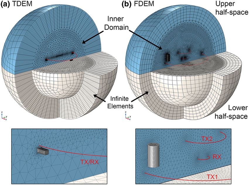
Effects of metallic system components on marine electromagnetic loop data 2255

                                            modelling. These procedures motivate the opportunity to design dedicated, compact,
                                            low-bias platforms and provide a solution for autonomous and remotely steered de-
                                            signs by minimizing their effect on the sensitivity of the controlled-source electromag-
                                            netic sensor.

                                            Key words: Electromagnetics, Modelling, Numerical study, Signal processing.

I N T RO D U C T I O N                                               also rely on a thoughtful construction and design, avoiding
                                                                     the use of electrically conductive materials in proximity of the
Over the last years, the marine controlled-source electromag-
                                                                     receiver to prevent bias on the measured data. Thus, a trade-
netic method (CSEM) exhibited large steps in the development
                                                                     off between rigid, cost-effective and non-conductive materi-
of new sensor platforms to meet the task of future resource ex-
                                                                     als (e.g. stainless steel versus fibreglass composites) has to be
ploration. In comparison to traditional geophysical and geo-
                                                                     found. In practice, the use of metals such as titanium is in-
chemical methods, applied to delineate mineralizations along
                                                                     evitable, considering the need of pressure housings for system
the seafloor, current investigations demand the detection of
                                                                     electronics and additional measuring or observation devices
extinct and buried mineral deposits. The contrast in electri-
                                                                     (e.g. conductivity/temperature/depth probes (CTD), magne-
cal conductivity between the valuable ores and the surround-
                                                                     tometers, altimeters, acoustic positioning, camera systems in-
ing host rock motivated the development of new CSEM de-
                                                                     ertial measurement units (IMU)). A possible approach is there-
vices. Even though von Herzen et al. (1996) and Cairns et al.
                                                                     fore to separate system electronics and sensor to a distance
(1996) conducted initial studies on electric measurements at
                                                                     where no bias is measurable. By the nature of marine off-
the Trans-Atlantic Geotraverse (TAG) hydrothermal mount,
                                                                     shore surveys, the time–cost–benefit equation is critical. This
it took over 10 years until severe interest in marine, high-
                                                                     favours the development of multi-sensor platforms or steer-
grade, polymetallic deposits and their exploration was fuelled
                                                                     able ROV/autonomous unmanned vehicle (AUV)-based de-
by rising resource prices. Kowalczyk (2008) performed first
                                                                     signs, to refine and complement the measured data set and en-
interdisciplinary studies, including bathymetric and magnetic
                                                                     hance geological interpretations (Kowalczyk, 2008; Lee et al.,
surveys and a remotely operated vehicle (ROV)-based coil ex-
                                                                     2016; Bloomer et al., 2018). Here, a spatial separation be-
periment, to search for conductive structures at the Solwara 1
                                                                     tween the transmitter/receiver and the metal components is
hydrothermal field. Swidinsky et al. (2012) studied the sensi-
                                                                     constrained by the extremely limited space, if not completely
tivity of transient loop sensors for submarine massive sulphide
                                                                     unfeasible. Hence, a certain degree of bias is inevitable in these
exploration. Since then, several devices have been applied for
                                                                     cases, which are relevant to active noise levels recognized by
massive sulphide mapping, including electrical and electro-
                                                                     several authors including Nakayama and Saito (2016) and
magnetic (EM) dipole systems (e.g. Gehrmann et al., 2019;
                                                                     Bloomer et al. (2018). A pure mapping approach is therefore a
Ishizu et al., 2019) and horizontal loop systems that offer a
                                                                     robust and fast way to identify larger conductivity anomalies
small footprint, high vertical resolution and compactness. GE-
                                                                     by analysing relative deviations from the background signal.
OMAR’s MARTEMIS time-domain electromagnetic (TDEM)
                                                                     Yet, this approach does not exploit the full potential of the
and the GOLDEN EYE frequency-domain electromagnetic
                                                                     method, which aims at the inversion of the measured data to
(FDEM) loop system, operated by Germany’s Federal Insti-
                                                                     derive physical parameter distributions and geological inter-
tute for Geosciences and Natural Resources (BGR), have been
                                                                     pretations. This requires sensitive measurements that are ca-
developed and deployed at various hydrothermal fields. Con-
                                                                     pable of delivering reliable, high-quality data sets. This study
ductive structures at the TAG and Palinuro Seamount (Hölz
                                                                     therefore assesses and quantifies the static effects of critical
et al., 2015) and in the German licence areas were successfully
                                                                     system components and evaluates their influence on the pro-
mapped for polymetallic sulphides at the Central Indian Ridge
                                                                     duced data sets and inversion results for the first time. Two
(Schwalenberg et al., 2016; Müller et al., 2018). Sensor oper-
                                                                     case studies of highly sensitive, marine CSEM systems with (1)
ations in mid-ocean ridge settings, at seamounts of complex
                                                                     time-domain and (2) frequency-domain coil sensors are anal-
bathymetry, and under harsh weather conditions, require rigid
                                                                     ysed to quantify their platform-immanent bias and to develop
and compact devices for safe on-board handling and deep-
                                                                     data calibration and system optimization strategies. The nu-
water surveying. However, especially loop–loop EM systems
                                                                     merical calculations, supported by field data, are carried out

© 2020 The Authors. Geophysical Prospecting published by John Wiley & Sons Ltd on behalf of European Association of
Geoscientists & Engineers., Geophysical Prospecting, 68, 2254–2270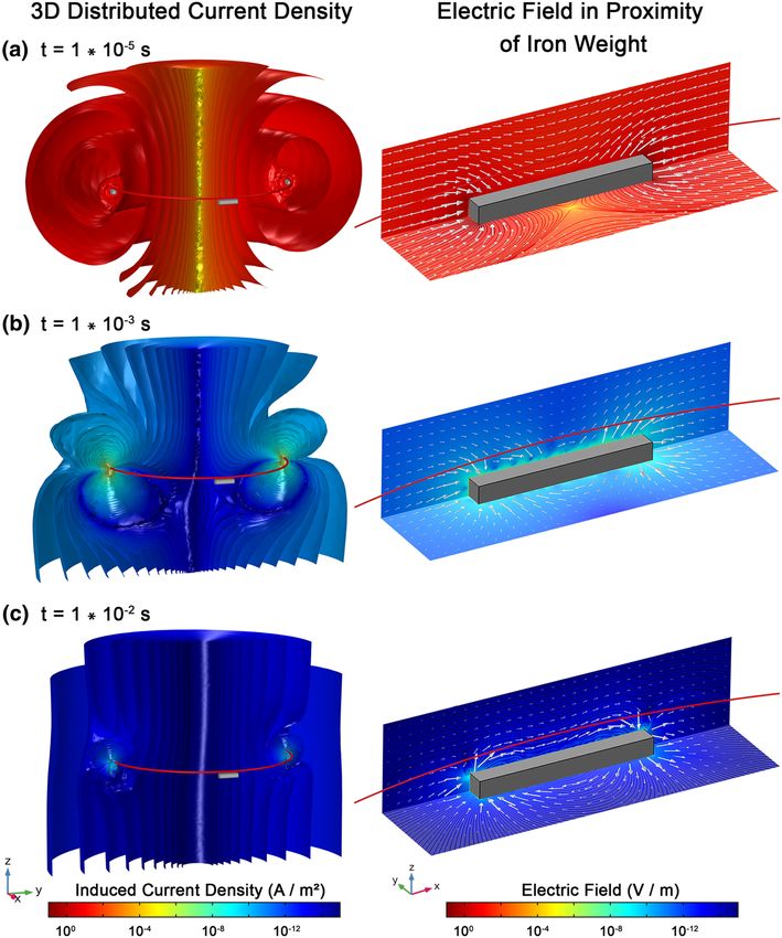
2256 K. Reeck et al.
self-potential (SP) electrodes are usually installed on the coil
frame. The instrument is operated at a flight height of 1–3
m above the seafloor which is frequently measured by an al-
timeter from the upper frame through the coil. Since 2015,
several surveys have been carried out on an annual basis, in-
cluding cruises to the Trans-Atlantic Geotraverse hydrother-
mal site in 2016, the Mediterranean Palinuro seamount off
Sicily in 2015 and 2017 and the Grimsey hydrothermal field
in 2018 and 2019 (Hölz et al., 2018). For all cruises, data were
successfully recorded, identifying the buried, electrically con-
ductive metal sulphite. Until 2017, metal corner connections
and iron weights were utilized as a cheap and durable solu-
tion to enhance the rigidity and handling of the coil frame.
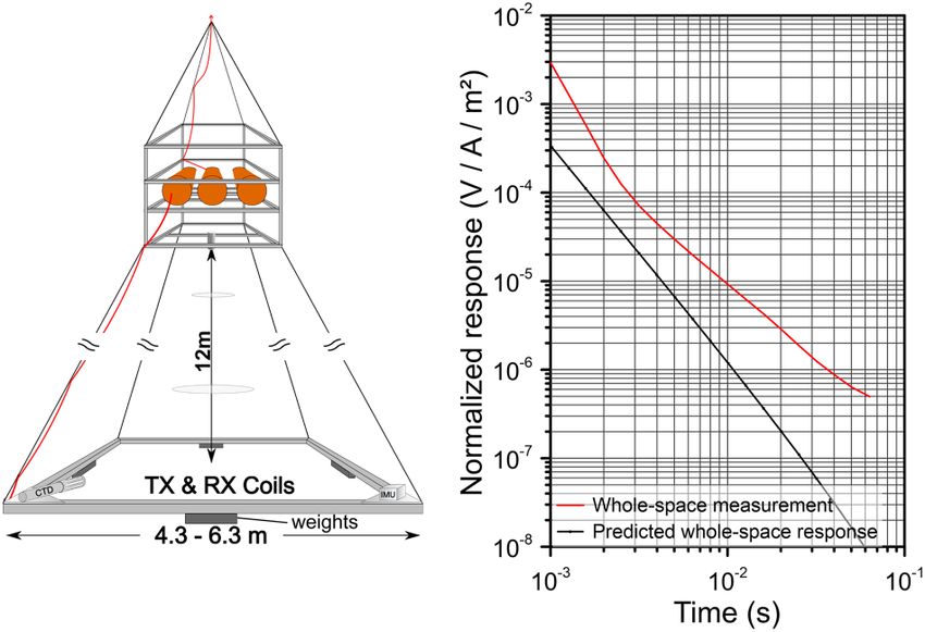
Figure 1 MARTEMIS TDEM system and (biased) data example: (a) However, these highly conducting elements also led to a signif-
Concept of GEOMAR’s MARTEMIS time-domain coil system with
icant, non-uniform and time-dependent offset in the measured
separated system electronics (upper frame) and the coincident-loop
sensor (lower frame) connected by long ropes. The conductive weights data, complicating the analysis substantially (Fig. 1b). This is-
were installed directly onto the coil frame as well as smaller, additional sue is now resolved through improvements on the fibreglass
sensors like a CTD and an IMU. (b) Biased data example of a station- structure and use of non-conducting barite weights. The af-
ary whole-space measurement in the water column during POS509 in fected data sets required a thorough post-processing and bias
2017.
removal prior to the inversion (e.g. Haroon et al., 2018). How-
ever, a scientific approval of the used calibration concept has
by finite element (FE) modelling in the commercially available remained pending up to this point and will be demonstrated
COMSOL Multiphysics suite, applicable to resolve both time in the following.
and frequency-domain quasi-static EM problems. The derived
bias factors for variable sensor configurations and visualiza-
FREQUENCY-DOMAIN SYSTEM
tions based on the computed current density distributions in
3D are especially useful when: (a) developing new or evalu- Federal Institute for Geosciences and Natural Resources’
ating present CSEM profilers in terms of high sensitivity/low (BGR’s) GOLDEN EYE frequency-domain coil system, devel-
bias, (b) analysing and calibrating existing data sets of other oped in 2012, features a more compact and rigid design: a
comparable devices to allow for the inversion and full inter- fibreglass structure carries the transmitter (TX) and receiver
pretation. (RX) coils as well as all titanium pressure housings (Fig. 2a).
The design enables the device to be used as a multi-sensor
platform, incorporating cameras with live link, a conduc-
TIME-DOMAIN SYSTEM
tivity/temperature/depth, a forward-looking sonar, a magne-
GEOMAR’s MARTEMIS system has been under successive tometer and a self-potential/induced polarization system. The
development since 2012 and trades a compact design for a compactness and monitoring capabilities provide the oppor-
distinct separation of up to 15 m between an upper fibre- tunity to easily land the system on the seafloor for station-
glass frame, holding most electric field distorting titanium, ary, high-resolution measurements. The electromagnetic sen-
system electronic pressure housings, and a lower frame, car- sor features a compensation (‘bucking’) coil that generates a
rying a coincident-loop transmitter (TX) and receiver (RX) magnetic cavity in place of the RX coil. This allows for sen-
coil (Fig. 1a). This rope-connected construction allows for a sitive measurements of in-phase and quadrature components
rapid adjustable, modular set-up based on a survey vessel’s while continuously transmitting up to 12 combined sine waves
specification. Usual coil sizes between 18.5 and 39.7 m2 lead in a frequency range from 10 to 10,000 Hz. The system pro-
to depth of investigations (DOI) between 30 and 50 m (Hölz vides approximately 20 m depth of investigations with high
et al., 2015). Depending on the target, a horizontal, electri- near-surface resolution.
cal dipole with two polarizations may be utilized instead of Similar to the MARTEMIS system, a bias was identi-
the coil to map resistive structures. Additional instruments, in- fied in the measured data over all frequencies of the in-
cluding a conductivity/temperature/depth probe, an IMU and phase and quadrature components (Fig. 2b). By submerging
© 2020 The Authors. Geophysical Prospecting published by John Wiley & Sons Ltd on behalf of European Association of
Geoscientists & Engineers., Geophysical Prospecting, 68, 2254–2270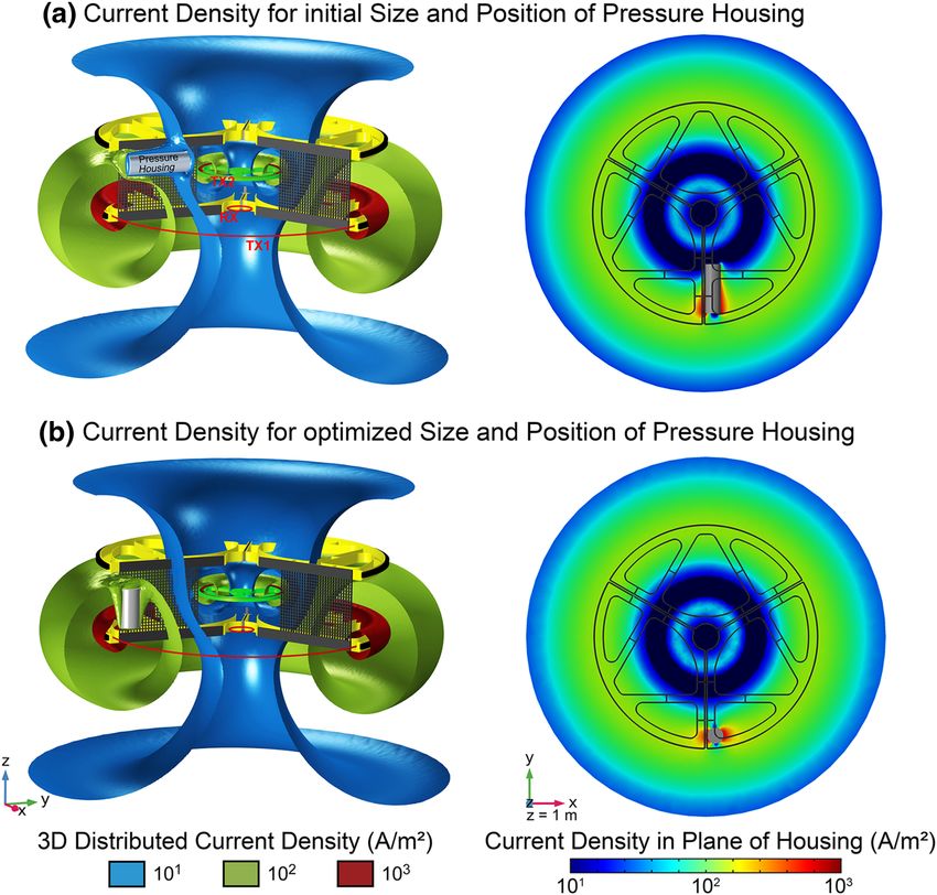
Effects of metallic system components on marine electromagnetic loop data 2257
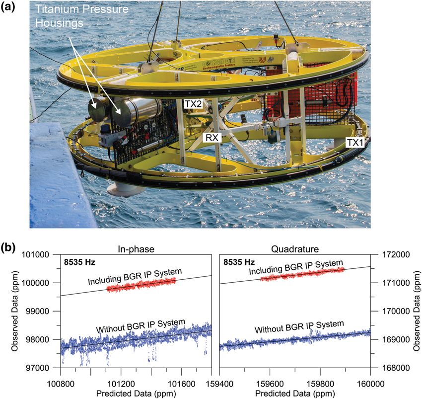
Figure 2 GOLDEN EYE FDEM system and (biased) data example: (a) GOLDEN EYE profiler deployed from RV Heincke. The FDEM system
consists out of a large transmitting (TX1) coil and a coplanar concentric receiving (RX) coil in the lower plane and an upper, elevated ‘bucking’
(TX2) coil in ensemble with an underwater sensing infrastructure. (b) Data example of a range of whole-space measurement in the water column
against the predicted responses based on CTD measurements during the INDEX2015 cruise for different setups. The BGR SP/IP system adds
two large titanium housings to the instrument that lead to the observed offset (red).
the GOLDEN EYE in a seawater pool with various configu- AC/DC module that solves Maxwell-Amperes law (equation
rations, it was experimentally proven that the distortions were (1) for time-domain electromagnetics, respectively, equation
related to the pressure housings in close proximity of the TX (2) for frequency-domain electromagnetics).
and RX coils. Thus, substantial post-processing and calibra-
∂D
tion was required to successfully analyse and invert the data ∇ × H − σE − − Je = 0, (1)
∂t
sets (Müller et al., 2018). Due to the nature of a compact
multi-sensor platform, positioning of pressure housings out of
∇ × H − σ E − jωD − Je = 0, (2)
the sensor’s range is not possible. Therefore, efficient calibra-
tion methods and system optimization strategies are required where σ denotes the electric conductivity, j denotes the imagi-
to minimize the biasing effects on the data and interpretation. nary number, H denotes the magnetic field, E denotes the elec-
tric field, B denotes the magnetic flux density, D denotes the
displacement current, ω denotes the angular frequency and Je
FINITE ELEMENT MODELLING IN COMSOL
denotes an external current density. Given the constitutive re-
M U LT I P H Y S I C S
lations for magnetically and electrically linear materials (equa-
The 3D forward modelling was conducted in COMSOL Mul- tions 3 and 4), this transforms into the governing equations (5)
tiphysics 4.3a and 5.3a using the magnetic fields physics of the and (6) for time and frequency domain that are solved for the
© 2020 The Authors. Geophysical Prospecting published by John Wiley & Sons Ltd on behalf of European Association of
Geoscientists & Engineers., Geophysical Prospecting, 68, 2254–2270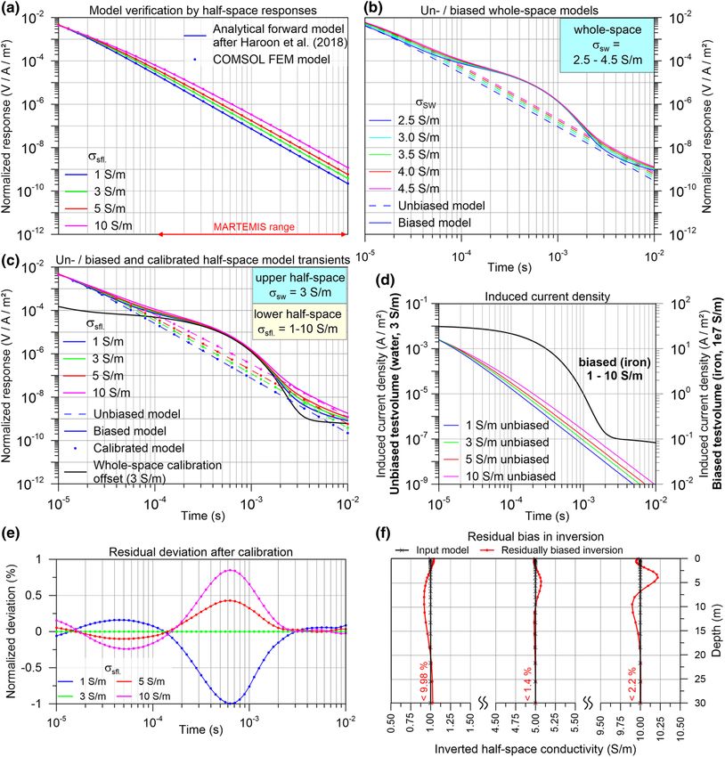
2258 K. Reeck et al.

Figure 3 Finite-element-model set-up for
(a) TDEM and (b) FDEM. Cross-section
of the finite element models. For the
inner computational domain, a tetrahe-
dral meshing is used and refined in ar-
eas of high field gradients and low skin
depths (e.g. coil area, red). For the out-
ermost area, an infinite elements domain
with swept mesh is used, which virtually
stretches the coordinates towards infinity
and dampens the fields.

magnetic vector potential A on a finite element (FE) grid (see        mum skin depth and therefore on the frequency and electrical
COMSOL 2017 for further details).                                     conductivity of the domain (Fig. 3). A spherical, inner com-
                                                                      putational domain serves as main model space. In the upper
B = μ0 μr H with μr = (1 + χm ) ,                             (3)
                                                                      half-sphere, all relevant objects of the device are parameter-
                                                                      ized, including the transmitter (TX)/receiver (RX) coils as well
D = ε0 εr E with εr = (1 + χe ) ,                             (4)     as weights or pressure housings. The lower half-sphere yields
where μ0 and ε0 denote the magnetic permeability and electric         the opportunity to assign a layered earth model and buried ob-
permittivity of free space, μr and εr denote the relative mag-        jects. Furthermore, a mesh refinement resolves the high field
netic permeability and electric permittivity, and χ m and χ e the     gradients in close proximity of the TX coils. The outer do-
magnetic and electric susceptibility.                                 main is meshed as ‘infinite elements’, used to dampen the fields
                                                                      by virtually stretching the elements to infinity and avoiding
    ∂A        ∂ 2A
σ      − ε0 εr 2 + ∇ × μ−1 −1
                        0 μr ∇ × A − Je = 0.                  (5)     any amplifying, diffusion-hindering effects. Prior to the bias
    ∂t        ∂t
                                                                      modelling, a series of tests were completed to verify the so-
                                                                  lution’s accuracy. Domain and mesh scaling/sensitivity tests
    jωσ − ω2 ε0 εr A + ∇ × μ−1 −1
                            0 μr ∇ × A − Je = 0.              (6)
                                                                      were conducted by analysing the influence of the domain and
     It is important to note that for the relevant conductiv-         mesh size.
ity and frequency range, the quasi-static approximation is as-
sumed so that the corresponding terms of the displacement
                                                                      TIME-DOMAIN 3D FINITE ELEMENT
current in equation (5) and (6) can be neglected.
                                                                      MODEL AND STUDIES
     Initial concepts of the FE models were designed as whole-
space and half-space solutions for an efficient, 2.5D axial-          The upper fibreglass frame of the MARTEMIS system is ne-
symmetric geometry to benchmark and verify the model                  glected in the 3D simulations, since experimental field testing
against analytical solutions and field data with low computa-         showed that the influence of the titanium housings is negligi-
tional costs. Subsequently, 3D models were developed, incor-          ble at a distance of over 15 m from the receiver (RX) coil. This
porating non-symmetric and more complex elements like pres-           simplifies the model due to the reduced size of the main com-
sure housings. Different domains are used to apply an ideal,          putational domain and results in significantly less degrees of
tetrahedral meshing on each component, based on the maxi-             freedom and computational costs. As a result, the model only

                    © 2020 The Authors. Geophysical Prospecting published by John Wiley & Sons Ltd on behalf of European Association of
                                                                      Geoscientists & Engineers., Geophysical Prospecting, 68, 2254–2270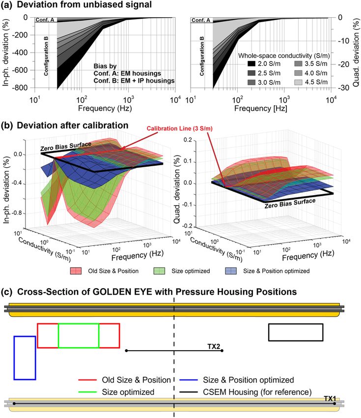
Effects of metallic system components on marine electromagnetic loop data 2259

consists of the transmitter (TX) coil, which also acts as a coin-                FREQUENCY-DOMAIN 3D FINITE
cident RX (Fig. 3a). For further simplification and symmetry,                    ELEMENT MODEL AND STUDIES
the coil is chosen to be circular with 4.85 m diameter and 40 A
                                                                                 The GOLDEN EYE sensor is based on the GEM-3 configura-
excitation current, reaching the equivalent TX moment of the
                                                                                 tion after Won et al. (1997), which is composed of two coaxial,
MARTEMIS’ square coil (4.3 m × 4.3 m, 40 A). Due to this
                                                                                 circular transmitting coils. A larger 3.34 m diameter transmit-
simplification, the initially used iron corners were neglected in
                                                                                 ter (TX1) with 60 A (peak–peak) and 8 windings generates
the model, considering their complex geometry. The modelled
                                                                                 the primary magnetic field, while a 1.0 m diameter elevated
bias is solely introduced by the four iron weights. A distance
                                                                                 ‘bucking’ coil (TX2) of 7 reverse windings is tuned to buck out
of 1 m to the seafloor is chosen to represent optimal measure-
                                                                                 the primary magnetic field at the 0.3 m diameter receiver (RX)
ment conditions. The induced voltage in the RX coil (Vind,Rx )
                                                                                 coil, located in the centre of the TX1 coil (Figs 2a and 3b). The
is subsequently obtained by integrating the time derivative of
                                                                                 transmitter (TX) coils are incorporated in the FE model, us-
the vertical magnetic flux density (Bz ) over the coil area, with
                                                                                 ing line currents. Pressure housings are implemented as cylin-
r being the radius and φ being the azimuth of the (circular)
                                                                                 drical cavity tubes with corresponding lengths, diameters and
coil:
                                                                                 wall thicknesses. The conductivity of the titanium cylinders
                                                                                 was set to 4.12 × 10⁶ S/m. The interior of each pressure tube

                      rRx           2π
                                         dBz (r, φ)                              was chosen to be air to resolve the effect of the pure titanium
Vind,   Rx   =−                                     dr dφ.                (7)
                  0             0           dt                                   body. The RX coil is simplified to a point probe, measuring the
                                                                                 vertical magnetic flux density at the common centre of TX1
                                                                                 and RX. The response is calculated by the ratio between the
      Vind,Rx is subsequently normalized by the TX current and
                                                                                 un-bucked primary field and the measured, induced secondary
coil area.
                                                                                 field in parts-per-million. For the actual instrument, a small
      For the upper half-space, a constant conductivity of 3 S/m
                                                                                 reference coil in the centre of the TX2 coil continuously mea-
was chosen to represent seawater conductivity. A high con-
                                                                                 sures the primary field intensity and is used to normalize the
ductivity of 106 S/m is assigned to the iron weights, yielding a
                                                                                 secondary field. Since the induced voltage of a coil is propor-
volume of 4000 cm3 each. Lower half-space (seafloor) conduc-
                                                                                 tional to the time derivative of the orthogonal magnetic flux
tivities are varied in a series of studies to simulate low (1 S/m)
                                                                                 through the (small) RX coil, a point probe is considered as
and high (5 and 10 S/m) conducting half-space and whole-
                                                                                 a suitable simplification. Prior to the model studies, a bench-
space responses.
                                                                                 marking was carried out by comparing the analytical solution
      Two basic studies were conducted:
                                                                                 to the solution of the point probes and the calculated induced
1. Whole-space modelling with varying conductivities from
                                                                                 voltage (Vind,Rx ) after Ward and Hohmann (1988) from the
2.5 to 4.5 S/m in steps of 0.5 S/m.
                                                                                 vertical magnetic flux density (Bz ) for the RX coil (equation
2. Half-space modelling with an upper half-space conductiv-
                                                                                 8) in 2.5D and 3D (Fig. 5):
ity of 3 S/m and variable lower half-space conductivities of 1,                                   rRx  2π
5 and 10 S/m.                                                                    Vind, Rx = −iω             Bz (r, φ) dr dφ.                    (8)
      A time-dependent solver was used in the specified time                                     0     0

range from 10−6 s to 10−2 s, with 10 steps per decade tak-                            Even though the full modelling of all coils is more elegant,
ing an average computational time of 30 min for a half-space                     the simplification yields an important time-saving aspect since
model on an Intel i7 8900k with 64 GB of RAM. To stabi-                          the degrees of freedom and therefore the computational time
lize the solutions, the built-in stabilized biconjugate gradient                 of the model are drastically reduced. This enables the model to
solver was optimized with custom, fixed time-stepping and                        run in a reasonable amount of time (45 min for a half-space
continuous Jacobian calculations (see COMSOL 2017 for fur-                       model with full frequency sweep on the Intel i7-8900k with
ther details). Since instable solutions and aliasing effects can                 64 GB of RAM).
arise from imprecise and automated (free) time-stepping and                           The following studies were conducted:
thus interpolated results of the solver, studies with refined time               1. Whole-space modelling with varying conductivities from 2
steps and larger time ranges (10−9 to 100 s, 20 steps/decade)                    to 4.5 S/m in steps of 0.5 S/m.
were carried out to control the solution. These numeric finite                   2. Half-space modelling with an upper half-space conductiv-
element models were compared with results from analytical                        ity of 3 S/m and lower half-space conductivities of 0.1, 1, 3, 5
1D models.                                                                       and 10 S/m.

© 2020 The Authors. Geophysical Prospecting published by John Wiley & Sons Ltd on behalf of European Association of
Geoscientists & Engineers., Geophysical Prospecting, 68, 2254–2270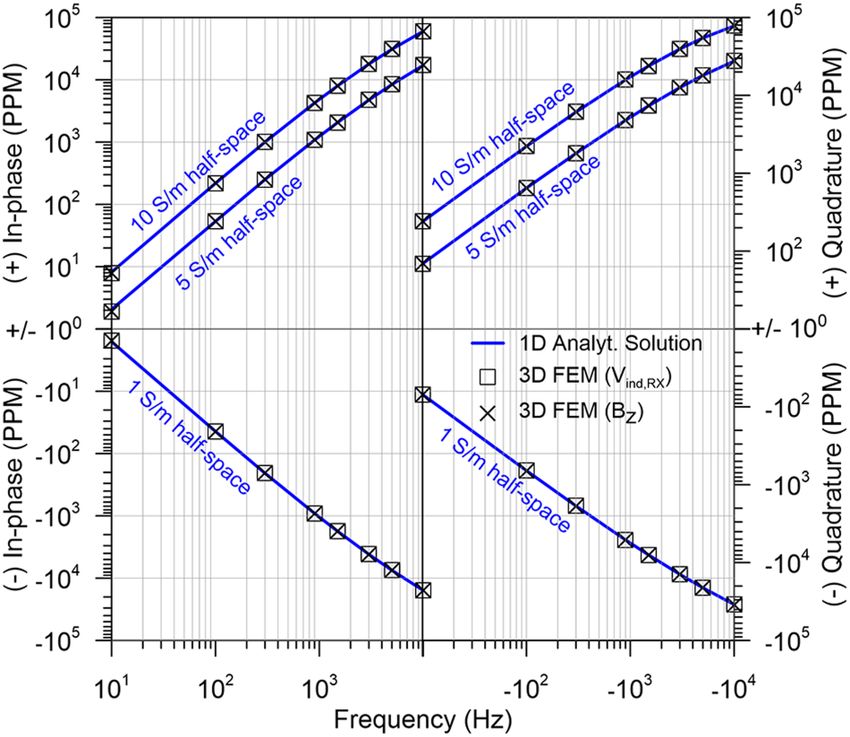
2260 K. Reeck et al.

     After result evaluation, additional optimization steps          (cf. Fig. 1b). The iron weights are therefore clearly confirmed
were carried out, including the re-dimensioning and reposi-          as a main source of bias, although the amplitude deviation is
tioning of the pressure housings. For the studies, a common          generally higher in the measured data. This difference is likely
frequency spectrum of the instrument with 30, 105, 285, 885,         due to the neglected iron edges in the modelling and therefore
2715 and 8535 Hz was swept, according to the set-up of a             a lower amount of conductive material in the sensor’s vicin-
previous survey. For frequency-domain electromagnetics, the          ity. However, the highest amplitude deviations occur at early
default configuration of the implemented stabilized biconju-         times, indicating the close proximity of the metal objects to
gated gradient solver was used in all studies.                       the coil. Further amplitude variations are caused by the sec-
                                                                     ondary electric fields produced through the decaying charge
                                                                     in the conductive weights. Therefore, the bias can be directly
R E S U LT S T I M E - D O M A I N                                   related to the change of the induced current density J in the
Verification of 3D finite element model by 1D analytical             specified volume of the weights (equation (9)).
forward model                                                        J = σ E.                                                      (9)
A three-dimensional time-domain electromagnetic model of                   For the background model (volume being water), the in-
the MARTEMIS system has been developed by using COM-                 duced current density depends on the lower half-space’s con-
SOL’s AC/DC magnetic fields module. While first models               ductivity (Fig. 4d, coloured lines). By changing the material
lacked the precision to match the 1D analytical solution, the        to iron, the current density increases drastically, leading to an
customization of the time-stepping solving algorithm solved          apparent decoupling from the lower half-space’s conductiv-
this issue. Afterwards the model was successfully verified           ity: a dependency between lower half-space conductivity and
against the 1D analytically calculated forward model (Fig. 4a):      induced current density is no longer visible and the resulting
the modelled transients for all half-space/whole-space models        calibration offset can be considered nearly static for the anal-
match the solution of the 1D solution in the analysed time           ysed range of 1 to 10 S/m (Fig. 4d, black line).
range of 10−5 to 10−2 s.

                                                                     Calibration of biased data by 1D analytical forward model
Introduction of the bias effect in 3D finite element model
                                                                     The independence from the sub-surface conductivity structure
The reproduction of the bias effect detected in the measured         offers the possibility to calibrate the sensor against a known
MARTEMIS data sets was achieved by introducing highly                whole-space conductivity model based on measured conduc-
conducting (106 S/m) iron weights into the 3D model. Figures         tivity/temperature/depth values. However, this approximation
4b and c illustrate the difference between biased and unbi-          can only be considered valid while the apparent decoupling
ased whole-space, respectively, half-space models. A high, but       between seafloor and the biasing object holds true, for exam-
varying deviation of up to 1.5 magnitudes from the original          ple, the conductivity contrast stays sufficiently large. A proof
transients (coloured dashed lines) can be observed in the com-       of this concept can be presented by calibrating biased data. To
puted time range for both whole-space and half-space models.         avoid further error sources found commonly in measured data
The separation between the biased and unbiased responses             sets, synthetic data for whole-space and half-space models are
can be observed in early times (between 10−5 and 10−4 s),            used.
and in the same range of time a separation between differ-                 A whole-space model is used as calibration measure-
ent half-space models is expected. Since this is one decade be-      ment, assuming a steady seawater conductivity of 3 S/m. The
low MARTEMIS’ earliest sampling time of 10−4 s, a recorded           ‘seafloor measurements’ models consist of the upper half-
transient is likely to be completely biased. The observable vari-    space with a seawater conductivity of 3 S/m and a lower half-
ation by the change in seawater conductivity is small due to         space with either 1, 5 or 10 S/m. These are considered as cases
the generally large amplitude of the bias effect, but becomes        of low conducting background sediments and high to very
more visible at later times (10−3 to 10−2 s). In this relevant       high conducting massive sulphides that meet the envisioned
time range, the different models are well distinguishable, but       application of the MARTEMIS system. To calibrate the syn-
still biased by a variation of approximately 0.5 S/m at mini-        thetic biased measurements (SWS,biased ), an unbiased system re-
mum. The biased modelled data correlate well with the biased,        sponse (SWS,unbiased ) for a whole space (WS) of known conduc-
measured whole-space data in terms of amplitude and timing           tivity is needed. This can be derived either from the 3D model

                   © 2020 The Authors. Geophysical Prospecting published by John Wiley & Sons Ltd on behalf of European Association of
                                                                     Geoscientists & Engineers., Geophysical Prospecting, 68, 2254–2270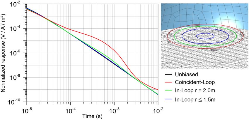
Effects of metallic system components on marine electromagnetic loop data 2261

Figure 4 Results of TDEM modelling: (a) TDEM verification of the FE model–derived solution against an analytical calculated forward model
for varying lower half-space conductivities. (b) Unbiased (dashed, coloured) and biased (solid, coloured) transients of the MARTEMIS system
for a set of whole-space conductivities ranging between 2.5 and 4.5 S/m. (c) Unbiased (dashed, coloured) versus biased (solid, coloured) model
responses for a set of varying lower half-space conductivities with 1, 3, 5 and 10 S/m. Subtraction of the unbiased whole-space (3 S/m) response
from the biased whole-space response results in the whole-space calibration offset (solid, black). This offset is used to calibrate all half-space
responses (dots, coloured). (d) Induced current density in the defined testvolume of a single iron weight with different material properties (water,
iron). In case of the testvolume being iron, a dependence of the current density on the lower half-space conductivities is no longer visible. (e)
The deviation between the calibrated and unbiased model responses after the calibration is considered as residual bias. (f) Inversion of these
residually biased half-space model responses. The input model was used as a starting model to avoid any Occam-related deviations (RMS ≤ 1,
error floor 1%). Due to the calibration the whole-space (3 S/m) response is perfectly calibrated while the 1, 5 and 10 S/m responses are showing
equivalent variations to the signal deviation in (e) of up to ±1% from the original signal in MARTEMIS’ significant time range of 10−4 to 10−2
s. This leads to errors of up to ∼10% for a non-conductive seafloor with 1 S/m, whereas higher conducting seafloor show lower offsets of ∼1.4%
for 5 S/m and 2.2% for 10 S/m. This favours the envisioned application of the MARTEMIS system targeting highly conductive ore deposits.

© 2020 The Authors. Geophysical Prospecting published by John Wiley & Sons Ltd on behalf of European Association of
Geoscientists & Engineers., Geophysical Prospecting, 68, 2254–2270
2262 K. Reeck et al.

or more easily from an available, time-saving, analytical solu-         Generally, the conductivity contrast is amplified as observed
tion. By subtraction, a time-dependent calibration offset S is          before: lower conductivities appear slightly less conductive,
calculated (equation 10):                                               while higher conductivities appear more conductive. While for
                                                                        the uppermost part of the profiles, the start of the observed
 S (t ) = SW S, biased − SW S, unbiased .                      (10)
                                                                        sign change can be recognized, the deeper part of the profile
     This whole-space calibration offset is now subtracted              remains almost unbiased. Depending on the purpose of the
from each biased transient, independently from the sub-                 instrument, this may influence the requested sensitivity of the
seafloor conductivity, to obtain the calibrated transients              sensor. In MARTEMIS’ case, of which purpose is to detect
(Fig. 4c, coloured point markers). The analysis of the resulting        large, inactive massive sulphide deposits with high conductiv-
‘calibrated’ signal shows similar transients compared with the          ities above seawater (3 S/m), a 2.5% deviation still results in
unbiased signal, thus proving the general applicability of the          the identification of the deposit. Thus, no severe consequences
concept.                                                                arise from this slight loss of sensitivity.

Residual bias in calibrated data                                        System optimization to reduce residual bias
Normalization of this calibrated response to the unbiased sig-          An optimization of the MARTEMIS system solely relates
nal for all seafloor measurements shows deviations less than            to the reduction of conductive elements in proximity of
0.5% for most of the time series, but ∼1% in the time range             the coincident transmitter and receiver coils. In 2018, the
of 10−4 to 10−3 s, which is in the magnitude of the expected            metal weights were simply replaced by non-conductive barite
minimum relative measurement error (Fig. 4e). Still, this addi-         weights and the metal edges by fibreglass composites, which
tional error source stacks with systematic and random errors            proved to be extremely durable during recent measurements.
and may influence the retrieved conductivity of the data set. A         Thus, conductive parts are completely eliminated from the
considerable relevance to an inversion result can be attributed,        lower frame and whole-space measurements are now in ex-
since the sign of the deviation is dependent on the conductivity        cellent agreement to the theoretical response.
contrast: in the time range of 10−4 to 10−3 s, lower conduc-
tive half-spaces will produce negative deviations from the un-
biased signal and vice versa. For the range of 10−5 to 10−4 s, a        R E S U LT S F R E Q U E N C Y - D O M A I N
sign change with lower amplitude can be observed. However,              Verification of 3D finite element model by 1D analytical
since this time range is not resolvable by the MARTEMIS sys-            forward model
tem, it is reasonable to deduce that the calibration will amplify
the measured conductivity contrast towards seawater.                    Comparing the finite element (FE) model responses against
                                                                        the 1D analytical solution shows the successful development
                                                                        of the 3D FE model. To illustrate this in Fig. 5, the whole-space
Influence of residual bias on inversion results                         response is subtracted from each half-space response and dis-
To quantify this residual influence, the calibrated responses of        played on a logarithmic scale: an excellent agreement is visible.
the biased half-space models were inverted for the time range           Both the response based on the calculated induced voltage in
of 10−4 to 10−2 s, using an Occam-inversion algorithm (Con-             the receiver (RX) coil (Vind,Rx ), as well as the solution based
stable et al., 1987) based on the 1D forward code of Swidin-            on vertical magnetic flux density derived from the central
sky et al. (2012). To avoid any Occam-based deviations, the             point probe (Bz ) show identical solutions. Due to the lower
input model was used as starting model for the inversion.               computational costs, the latter solution is used in all further
Figure 4(f) shows the inversion results for each residually             calculations.
biased half-space model after calibration. Comparable to
the normalized deviations of the calibrated model responses
                                                                        Introduction of the bias effect in 3D finite element model
in Fig. 4(e), small variations are visible that depend on the
conductivity of the lower half-space: the 1 S/m half-space ex-          The results of the frequency-domain whole-space model show
hibits the highest deviation by ∼10% at a depth span of 5               an effect similar to the one observed in the whole-space
to 15 m. The conductive half-spaces 5 and 10 S/m show de-               measurements of the INDEX2015 survey (cf. Fig. 2b). Espe-
viations of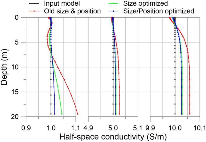
Effects of metallic system components on marine electromagnetic loop data 2263

                                                                         A are 20 cm shorter than the added housings in configuration
                                                                         B and are placed further to the outside of the frame (see Fig. 6c
                                                                         for size reference).

                                                                         Calibration of biased data by 1D analytical forward model

                                                                         To eliminate the bias without the removal of the necessary
                                                                         housings, calibration techniques are required. One of the ap-
                                                                         plied techniques is based on the dependency between con-
                                                                         ductivity and observed response (Fig. 2b): a frequency- and
                                                                         phase (respectively in-phase/quadrature)- specific calibration
                                                                         against the forward-calculated (predicted) response is com-
                                                                         monly used to eliminate system-immanent deviations between
                                                                         the analytical model and measured data to allow the inver-
                                                                         sion of the data. As shown by Müller et al. (2012) and Baasch
                                                                         et al. (2015), this can be achieved by the measurement of the
Figure 5 FDEM verification; FDEM verification between the 3D FE          seawater’s conductivity via conductivity/temperature/depth
models and the 1D analytical solution for a set of relative half-space   probes during a survey, used to create a database of (bi-
responses of 1, 5 and 10 S/m: the whole-space response of 3 S/m is
                                                                         ased) whole-space measurements (SBiased ) and corresponding
subtracted and a positive/negative logarithmic scale is used to allow
                                                                         forward-calculated analytical solutions (SCTD ) for the span of
for a better comparison. The signal of the induced voltage in the coil
corresponds to the signal of the Bz component in the centre point of     measured seawater conductivities (equation 11). By linear re-
the coil (point probe), allowing for a simplification of the model and   gression, a complex frequency (f)-dependent multiplier (A)
reducing computational time.                                             and offset value (B) are calculated and used to calibrate the
                                                                         data set afterwards:
self-potential/induced polarization (SP/IP) system results in a
                                                                         Sbiased f = A f SCTD f + B f .                             (11)
major deviation from the initial configuration (Fig. 6a). The
bias of an added pressure housing differs by (a) the in-phase                Limitations of the procedure arise from the fact that
or quadrature component, (b) the chosen frequency and (c)                an optimum sensor calibration is achievable only when the
the conductivity of the surrounding whole space. Configu-                conductivity of the surrounding is known and homogeneous.
ration A, yielding the basic set-up of GOLDEN EYE with                   The true conductivity of the seafloor is generally unknown
two smaller electromagnetic housings to perform controlled-              and may deviate in a large range of < 0.1 S/m for resistive
source electromagnetic method measurements, leads to a bias              rocks like basalts to over 10 S/m for highly conducting ore
of approximately 50% in the low-frequency in-phase com-                  deposits.
ponent and 2.5% in the low-frequency quadrature compo-
nent, both decreasing towards higher frequencies. The in-
                                                                         Residual bias in calibrated data
fluence of the conductivity is related to the conductivity
contrast between seawater and the pressure housings. The                 Comparable to the time-domain electromagnetic evaluation,
bias increases with higher contrasts and therefore lower                 we examine the residual bias effects by the variation of the
conductivities.                                                          lower half-space’s conductivity (0.1, 1, 5 and 10 S/m) in
      Configuration B, which adds two additional, larger pres-           the model while calibrating the response with a whole-space
sure housings to the system for SP/IP measurements, multiplies           measurement of 3 S/m. Figure 6(b) illustrates the residual
the bias effect by a factor of 16, while the overall characteris-        bias as a surface in a conductivity-frequency space (red sur-
tics remain constant. Considering the pure titanium volume of            face). The overall bias is effectively reduced by the calibra-
the housings, which yields about 6300 cm3 for configuration              tion up to zero where the 3 S/m whole-space conductivity
A and approximately a threefold volume for configuration B,              is reached. Deviating from this line, a residual bias remains
this effect does not simply scale with the pure titanium mass. It        for all other conductivities. For the in-phase components,
is more likely connected to the overall distribution of titanium         the initial effect in the uncalibrated data is reduced drasti-
between the TX and RX coils. The housings in configuration               cally to ∼1%, showing a decrease towards a sign change

© 2020 The Authors. Geophysical Prospecting published by John Wiley & Sons Ltd on behalf of European Association of
Geoscientists & Engineers., Geophysical Prospecting, 68, 2254–2270
2264 K. Reeck et al.
Figure 6 FDEM bias and calibration of the GOLDEN EYE. (a) Deviation from the unbiased whole-space signals for a set of different whole-
space conductivities and the two configurations of the device used during the INDEX2015 cruise. Configuration A represents the GOLDEN
EYE minimal set-up with two (smaller) titanium housings used for the EM soundings. Configuration B includes the SP/IP system, represented by
two additional, significantly larger titanium pressure housings. Thus, the bias effect is significantly larger. (b) Results of the system calibration
as residual bias surfaces in a conductivity–frequency–space for the initial set-up (red) and two optimization steps (green, blue). The reduction
of size (green) and the repositioning of the housing (blue) significantly reduce the amount of residual bias. The zero-bias-calibration line for 3
S/m is indicated as red line, while the optimum zero-bias-surface is illustrated in black. (c) Cross-section of the GOLDEN EYE indicating the
different set-ups during the optimization process. The black box illustrates the size of one of the EM housings for reference needed to operate
the system.
in the mid-frequency range and then rising up to 0.1% for System optimization to reduce residual bias
the high frequencies. The quadrature component shows an
With these results, approaches for a system optimization were
equivalent reduction ∼0.1% decreasing further towards lower
gathered, leading to (a) a possible reduction in size of the
frequencies.
pressure housings and (b) the resulting possibility to shift the
© 2020 The Authors. Geophysical Prospecting published by John Wiley & Sons Ltd on behalf of European Association of
Geoscientists & Engineers., Geophysical Prospecting, 68, 2254–2270Effects of metallic system components on marine electromagnetic loop data 2265
conducting half-spaces by approximately 50% (Fig. 7, blue
and green line).
DISCUSSION
The proposed calibration procedure yields an adequate ap-
proach to remove the larger part of the platform-immanent
bias. We have shown that the remaining, residual bias is small
enough to successfully invert the data and to produce rea-
sonable results even though deviations remain. Whether these
residuals are acceptable mainly depends on the envisioned ap-
plication, sensitivity and resolution requirements of a device.
For both MARTEMIS and GOLDEN EYE, a residual uncer-
Figure 7 Influence of residual bias on the inversion; 1D Inversion re- tainty of 1% to 2% for higher conducting cases, respectively,
sults of the residually biased half-space responses of 1, 5 and 10 S/m
≤ 0.1 to 0.2 S/m is rather negligible, considering the extremely
(RMS ≤ 1). Comparable with the TDEM results, the un-optimized
deviation is highest for the lowest conductivity by ∼10% (0.1 S/m),
inhomogeneous structure with large conductivity contrasts of
followed by the 10 S/m response by ∼0.6% (0.6 S/m). Due to the low- a massive sulphide deposit. In comparison, a surficial sedi-
est conductivity contrast towards the calibration point of 3 S/m, the ment mapping device, like the NERIDIS benthic profiler with
5 S/m response yields the lowest relative deviation of ∼0.4% (0.25 a smaller, comparable sensor to the GOLDEN EYE (Müller
S/m). The system optimization reduces the maximum bias to 1% (1 et al., 2012), would suffer severely from similar bias offsets.
S/m), 0.02% (5 S/m) and 0.025% (10 S/m).
Nonetheless, some persistent issues need to be addressed.
The most obvious is the loss of sensitivity by using an ap-
position of the pressure housings to an optimum position proximation to calibrate the data. Considering the maximum
(Fig. 6c). While option (a) targets the overall titanium mass deviation of the biased signals after calibration of about 1%
in the configuration, option (b) relates to the geometric dis- (Figs 4e and 6b), this systematic yet unknown error in terms
tribution of the titanium in relation to the coils. Both the size of amplitude and sign stacks with the random noise level of
reduction (green surface) and repositioning, by rotating the the instrument, leading to an approximate twofold of the un-
housing by 90° and moving it as far away from the RX as certainty. When respecting this larger error floor during the
possible (blue surface), effectively leads to a further reduction inversion by normalizing the data to this increased error, con-
of the bias (Fig. 6b), while the general characteristics of the ductivity contrasts are harder to resolve and sensitivity is lost.
bias surfaces remain. However, disregarding this error will lead to the systematic
over- or underestimation of the seafloor conductivity. In time
domain, even an enhancement of the measured contrast can
Influence of residual bias on inversion results
be predicted in the relevant time range, caused by the am-
To assess the influence of the initial bias and the optimiza- plification of this effect (Fig. 4e and f). On the other hand,
tion steps on the inversion process, the residually biased signal dynamic variations of this bias caused by moving conductive
of each step is inverted by an analytical 1D forward model- system components due to structural weaknesses during a sur-
driven inversion routine (Baasch et al., 2015). Corresponding vey will produce unpredictable time-dependent anomalies that
to the higher penetrating low-frequency in-phase component, are impossible to calibrate by the proposed method. While for
the deviation from the initial forward response is highest with static seafloor measurements this effect may be eliminated by
>10% for the highest penetration depths of 20 m, but also landing the device, a possible ship-induced heaving motion in
dependent on the half-space’s conductivity (Fig. 7, red line). the water column during the calibration measurements or a
Here the higher conducting half-spaces show lower deviations more efficient flying mode close to the seafloor is problem-
of 0.5% (5 S/m) respectively 6% (10 S/m), emphasizing higher atic. At this point, the importance of the calibration measure-
conducting targets. Following the results of the residual bias ments during the survey has to be stressed. The measurement
calculations, the optimization steps lead to a significant im- of a known environment is required, which basically reduces
provement of the inversion results by reducing the deviations the possible calibration points to the water column of known
for the low conductive half-space by ∼90% and for the higher conductivity and sufficient extent that exceeds the depth of
© 2020 The Authors. Geophysical Prospecting published by John Wiley & Sons Ltd on behalf of European Association of
Geoscientists & Engineers., Geophysical Prospecting, 68, 2254–22702266 K. Reeck et al.
Figure 8 Distortion of the generated ring current as 3D cut-away diagram (left) and horizontal plane view (right) in frequency domain (1000
Hz). (a) Deformation of the induced current density near the initially used titanium pressure housing. The induced ring current is channelled
towards the higher conducting object as path of lowest resistance which forms local extrema. (b) The deformation of the induced current density
is reduced due to the optimization of the pressure housing by resizing it and rotating it into a vertical orientation.
investigations (DOI) of the instrument. Strong thermohaline sible for cases when metallic components are not completely
layering of the water column can be detected by conductiv- inevitable. Here, the optimization procedure for the GOLDEN
ity/temperature/depth measurements during the diving phases EYE showcased an important aspect: the signature of metal-
and needs to be respected by a layered forward model in pro- lic components is not solely related to the inductive coupling
cessing. Time-varying layering in coastal areas needs to be and thus does not simply scale with the amount of conduc-
countered by multiple calibration points, covering the com- tive material used. It is also affected by the channelling of the
plete survey. Too sparse calibration points that hardly cover generated ring current through the higher conducting object,
the range of upper half-space conductivities during seafloor leading to a conductive coupling effect that influences the geo-
measurements, as well as bias sources in range (e.g. ships), will metrical distribution of the secondary fields and ultimately the
lead to offsets and an invalid calibration. This usually results measured response. While the inductive effect is related to the
in the systematic over- or underestimation of the inverted con- volume of conductive material and the magnetic flux density
ductivity section. Therefore, a practical way to deal with cali- as a function of distance to the source, the conductive effect
bration measurements is to include them at each start and end can be attributed to the geometrical distribution of the con-
of a profile, leading to a large database of calibration points ductive material near the sensor. The placement of the metallic
that can handle occasional imprecise measurements as well as pressure housings in areas of steep E-field gradients leads to
seawater conductivity variations and drift effects. the production of large, local extrema due to the current chan-
Considering these limitations, optimized platforms are nelling, and thus high offsets in the measured signal (Fig. 8a).
the way forward to keep the immanent bias as low as pos- Moving the housing to a more homogeneous area results in
© 2020 The Authors. Geophysical Prospecting published by John Wiley & Sons Ltd on behalf of European Association of
Geoscientists & Engineers., Geophysical Prospecting, 68, 2254–2270Effects of metallic system components on marine electromagnetic loop data 2267
Figure 9 Distortion of the generated current density as 3D cut-away diagram (left) and the distribution of the electric field near the iron weights
(right) in time domain. At 10−6 s, (a) the current density distribution (left) is essentially dominated by the induced ring current, which leads to
a channelling of the electric field through the higher conducting body and the charge up of the weight (right). Subsequently and represented by
10−3 s (b) and 10−2 s (c), the charged-up weights start to produce secondary, dipole-like fields (right), which lead to the distortion of the current
density (left). Note that the central area of the coil still shows a homogeneous current density distribution.
smaller local extrema with less influence on the measured sig- ring current. At 10−5 s, the channelling of the ring current
nal, even though the inductive effect may increase (Fig. 8b). through the conductive object is visible and comparable to
However, the repositioning of a housing into areas of low field the frequency-domain electromagnetic case, leading to the ob-
gradients away from the sensitive receiver (RX) will reduce the served increase of the induced current density, indicating the
inductive effect and may be considered if compactness is not charge up of the object (Fig. 9a). In the surrounding volume,
required. the generated ring current still dominates, while no offset is
In the time-domain case, the same effects are visible visible in the signal. Subsequently, the distributed current den-
in early times but now also relate to the decaying induced sity starts to change significantly. The charged up weights
© 2020 The Authors. Geophysical Prospecting published by John Wiley & Sons Ltd on behalf of European Association of
Geoscientists & Engineers., Geophysical Prospecting, 68, 2254–22702268 K. Reeck et al.
A further decrease to 0.5 m does not yield any further im-
provement. While a calibration is still necessary for this case,
the lower bias will lead to a numerically more stable offset cal-
culation. The difference between the biased and unbiased re-
sponse becomes smaller and the influence of imprecise calibra-
tion measurements decreases. However, possible drawbacks of
a smaller RX coil in terms of a lower signal-to-noise ratio and
thus a lower DOI need consideration, as well as the structural
more complex set-up.
Figure 10 Comparison between coincident-loop and in-loop re-
sponses in time domain. Biased whole-space responses are calculated
CONCLUSION
for different in-loop RX configurations. Due to the less distorted cen-
tre area of the coil, smaller RX areas show a lower bias, even though The observed bias effects in marine controlled-source elec-
no further improvements are visible below a radius of 1.5 m.
tromagnetic method (CSEM) data have been successfully re-
traced to conductive objects in close proximity to the receiver
produce local, dipole-like anomalies by the slower decaying (RX) for both time- and frequency-domain cases. Numerical
charge that distorts the decaying ring current and, thus, the modelling showed how highly conducting metal components
signal (Fig. 9b). This effect is dominant up to 5 × 10⁻³ s when change the response as a function of the surrounding seawater
the secondary fields start to decrease and the current density and seafloor conductivity. A primary calibration of the mea-
distribution normalizes (Fig. 9c). sured data against the predicted response of the measured sea-
Even though the effect was removed for the MARTEMIS water conductivity can be considered as a valid approach to
system by replacing the weights and edges with non- remove a substantial part of the bias for both time and fre-
conductive materials, we can propose an optimization strat- quency domain, enabling an inversion of the data and pro-
egy for more complex cases where this may not be feasible. ducing reasonable results. However, a residual bias remains as
Considering AUVs, ROVs or any other dedicated multi-sensor a function of seafloor conductivity and time respectively fre-
platform, it is unlikely to replace or move initially mounted in- quency. In our numerical case studies, we detected maximum
struments and parts in favour of the controlled-source electro- bias levels of 1% to 2% after calibration, approximately dou-
magnetic method (CSEM) sensor. Nakayama and Saito (2016) bling the estimated uncertainty of the devices. After inverting
discussed and tested two additional configurations to avoid this calibrated data, this accounts for 0.1 to 0.2 S/m devia-
noise in their measured data, by separating the remotely oper- tion. For higher conductivities and conductivity contrasts to-
ated vehicle from the sensor, using a towed system and using wards the background material, these values become increas-
their CSEM sensor as a deployable station. Another common ingly negligible, favouring the intended usage in ore deposit
approach would certainly be to separate the RX from the dis- exploration. Since the seafloor conductivity is generally not
turbed near field in proximity of the transmitter (TX), by mov- known, but the objective of the inversion process, this resid-
ing it to the undisturbed far field. Still these options drastically ual bias cannot be removed by calibration procedures without
increase costs and efforts while sacrificing the compactness of significant effort (e.g. ground truthing). For these cases, opti-
the device. Another remaining, more elegant optimization ap- mization approaches yield the possibility of a further reduc-
proach is therefore to modify the TX/receiver (RX) geometry tion of this platform-immanent bias. Redesigning and repo-
by avoiding distorted field areas in the integration area of the sitioning essential conductive system components into bias-
coil. Hence, we can utilize the more homogeneous field dis- minima results in less disturbance of the distributed current
tribution, found towards the centre of the MARTEMIS sys- density at the RX coil. Hence, we regard this as the way for-
tem, avoiding the local anomalies in proximity of the TX coil ward to remove a considerable part of the platform-immanent
(Fig. 9). Accordingly, this would translate into changing from bias, and to design and build compact, multi-sensor platforms
a coincident loop to a central in-loop configuration with a including CSEM sensors without sacrificing too much of the
smaller RX radius. To test this approach in our model, we re- sensor’s sensitivity. At this point, a careful evaluation between
duced the RX radius stepwise, to analyse the effect on the bias the benefits and the impact of additional sensors and de-
in a 3 S/m whole-space environment (Fig. 10). We found that vices needs to be carried out since every conductive compo-
an in-loop RX radius of 1.5 m reduces the bias to a minimum. nent still increases the immanent bias level. In case of existing
© 2020 The Authors. Geophysical Prospecting published by John Wiley & Sons Ltd on behalf of European Association of
Geoscientists & Engineers., Geophysical Prospecting, 68, 2254–2270You can also read