Supporting Spatial Management of Data-Poor, Small-Scale Fisheries With a Bayesian Approach
←
→
Page content transcription
If your browser does not render page correctly, please read the page content below
ORIGINAL RESEARCH
                                                                                                                                                 published: 01 July 2021
                                                                                                                                       doi: 10.3389/fmars.2021.621961

                                            Supporting Spatial Management of
                                            Data-Poor, Small-Scale Fisheries
                                            With a Bayesian Approach
                                            Jennifer Rehren 1* , Maria Grazia Pennino 1 , Marta Coll 2 , Narriman Jiddawi 3 and
                                            Christopher Muhando 4
                                            1
                                              Centro Oceanográfico de Vigo, Instituto Español de Oceanografía (IEO), Vigo, Spain, 2 Institute of Marine Science, Spanish
                                            National Research Council (ICM-CSIC), Barcelona, Spain, 3 Institute of Fisheries Research MALNF, Zanzibar, Tanzania,
                                            4
                                              Institute of Marine Sciences, University of Dar es Salaam, Zanzibar, Tanzania

                                            Marine conservation areas are an important tool for the sustainable management of
                                            multispecies, small-scale fisheries. Effective spatial management requires a proper
                                            understanding of the spatial distribution of target species and the identification of its
                                            environmental drivers. Small-scale fisheries, however, often face scarcity and low-quality
                          Edited by:
                                            of data. In these situations, approaches for the prioritization of conservation areas need
                      Chiara Piroddi,
          Joint Research Centre, Italy      to deal with scattered, biased, and short-term information and ideally should quantify
                     Reviewed by:           data- and model-specific uncertainties for a better understanding of the risks related
                     Marie Etienne,         to management interventions. We used a Bayesian hierarchical species distribution
        Agrocampus Ouest, France
                   Andrea Pierucci,
                                            modeling approach on annual landing data of the heavily exploited, small-scale, and
   COISPA Tecnologia & Ricerca, Italy       data-poor fishery of Chwaka Bay (Zanzibar) in the Western Indian Ocean to understand
                  *Correspondence:          the distribution of the key target species and identify potential areas for conservation.
                       Jennifer Rehren
                                            Few commonalities were found in the set of important habitat and environmental
                jen.rehren@gmail.com
                                            drivers among species, but temperature, depth, and seagrass cover affected the spatial
                  Specialty section:        distribution of three of the six analyzed species. A comparison of our results with
        This article was submitted to
                                            information from ecological studies suggests that our approach predicts the distribution
        Marine Fisheries, Aquaculture
               and Living Resources,        of the analyzed species reasonably well. Furthermore, the two main common areas
              a section of the journal      of high relative abundance identified in our study have been previously suggested by
         Frontiers in Marine Science
                                            the local fisher as important areas for spatial conservation. By using short-term, catch
         Received: 27 October 2020
           Accepted: 11 June 2021           per unit of effort data in a Bayesian hierarchical framework, we quantify the associated
           Published: 01 July 2021          uncertainties while accounting for spatial dependencies. More importantly, the use of
                             Citation:      accessible and interpretable tools, such as the here created spatial maps, can frame a
      Rehren J, Pennino MG, Coll M,
                                            better understanding of spatio-temporal management for local fishers. Our approach,
   Jiddawi N and Muhando C (2021)
     Supporting Spatial Management          thus, supports the operability of spatial management in small-scale fisheries suffering
  of Data-Poor, Small-Scale Fisheries       from a general lack of long-term fisheries information and fisheries independent data.
          With a Bayesian Approach.
           Front. Mar. Sci. 8:621961.       Keywords: small-scale fisheries, spatio-temporal management, Chwaka Bay, Western Indian Ocean region, coral
    doi: 10.3389/fmars.2021.621961          reefs, seagrass, Bayesian hierarchical model

Frontiers in Marine Science | www.frontiersin.org                                  1                                               July 2021 | Volume 8 | Article 621961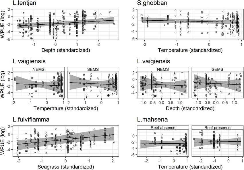
Rehren et al.                                                                                              A Bayesian Approach for Data-Poor Fisheries

INTRODUCTION                                                                 important to better understand the risks related to management
                                                                             interventions. Bayesian hierarchical species distribution models
Small-scale fisheries employ over 90% of the world’s capture                 are well suited for this purpose because they allow for a more
fishers (FAO., 2015, 2018) and are the major livelihood and                  accurate estimation of uncertainty, given that observed data
protein suppliers in many coastal communities around the world               and model parameters can be considered as random variables
(Chuenpagdee, 2011; Belhabib et al., 2015; Teh and Pauly,                    (Banerjee et al., 2004).
2018; Loring et al., 2019; Salas et al., 2019). It is believed that             We use a Bayesian hierarchical species distribution modeling
well-managed small-scale fisheries can contribute to poverty                 approach on landing data from different fishing gears collected
alleviation and food security (Bene et al., 2007; Purcell and                in 2014 to assess and predict the distribution range of key target
Pomeroy, 2015). However, assessing and managing these fisheries              species of Chwaka Bay. We identify common environmental
is challenging given the large number of species caught and                  drivers of distribution and areas of overlapping high relative
the adaptive behavior of fishers in space, time, and fishing                 abundance to prioritize potential conservation areas. The
methods (Wiyono et al., 2006; Salas et al., 2007; Daw, 2008).                analyzed species represent key target resources found in fisheries
The lack of alternative livelihoods and the strong resource                  catches throughout the Western Indian Ocean. Thus, our results
dependency of many small-scale fishing communities impede                    serve as baseline information for future studies in the region.
common management measures such as total allowable catches
or effort regulations (Pomeroy, 2012). Within the context of a
global agenda to protect 10% of coastal and marine ecosystems                MATERIALS AND METHODS
through area management by 2020 (CBD, 2010), many tropical
countries attempt to manage their coastal areas through different            Study Area
use-zones (Wells et al., 2007; De Santo, 2013).                              Chwaka Bay is a semi-enclosed bay-system located on the East
    Such an example is found in Zanzibar (Tanzania), where most              Coast of Zanzibar (Tanzania) (Figure 1). The bay is relatively
of the coastline has been designated a conservation area ranging             shallow, with depths up to 20 m in the outer borders and
from general use zones to locally managed partially protected and            some parts of the bay falling dry during low tide. The sea
privately managed no-take areas (McLean et al., 2012; Rocliffe               surface temperature ranges from 25 to 31◦ C and salinity from
et al., 2014). Zanzibar has achieved international targets by                35h at the bay opening to 26h in the bay proper (Jiddawi
protecting 11% of its continental shelf, but a rapid appraisal by            and Lindström, 2012). Strong tidal currents, with a mean tidal
regional experts estimated that only 25% of the coral reef MPAs              range of 3.2 m (Nyandwi and Mwaipopo, 2000), cause high
are effective (Rocliffe et al., 2014). Chwaka Bay on the east coast          turbidity in the bay by stirring up sediments (Gullström et al.,
of Zanzibar is an important, year-round fishing area, which is               2006). The north-eastern (November–March) and south-eastern
part of Zanzibar’s large Mnemba Island Marine Conservation                   (April–October) monsoons drive the bay’s climate, with the
Area management plan (MIMCA) (McLean et al., 2012). But                      latter showing stronger winds, longer rain periods, and lower
compliance with mesh-size and gear regulations is low (de la                 temperatures (Shaghude et al., 2012). The bay consists of a large
Torre-Castro and Lindström, 2010; Wallner-Hahn et al., 2016),                mangrove forest on the southern shore, dense seagrass meadows
making the bay a general use zone. A long history of intense                 throughout the bay, and a fringing reef at the bay opening. These
exploitation (de la Torre-Castro and Rönnbäck, 2004; Rehren                  habitats form a continuum through particulate organic matter
et al., 2018a), an increase in fishing effort (de la Torre-Castro            exchange (Mohammed et al., 2001) and tidal, seasonal, foraging,
and Lindström, 2010; Department of Fisheries Development.,                   and ontogenetic migration of fish (Gullström et al., 2012).
2016), the use of illegal gears, and spatial use-conflicts (de la                The diversity of habitats and the protection from wave energy
Torre-Castro and Lindström, 2010) have led to concerns for                   through the fringing reef give rise to a highly productive,
the sustainability of Chwaka Bay’s fisheries. In a participatory             year-round fishing area surrounded by several fishing villages
workshop in 2016, invited fishers advocated for implementing                 (Figure 1). The local community highly depends on the
a no-take zone to combat the decrease in their catches and the               fisheries’ resources for income and protein supply (Jiddawi and
reoccurring user conflicts (Rehren, 2017).                                   Lindström, 2012). The fishery targets multiple species ranging
    However, a prerequisite for the success of such no-take zones            from invertebrates (e.g., sea cucumber, octopus), reef- and
is to understand the spatial distribution of target species and              seagrass-associated fish (e.g., parrotfish and rabbitfish) to large
identify its environmental drivers. While the people of Chwaka               pelagic species (e.g., mackerels and jacks). The main fishing gears
Bay strongly depend on fisheries resources for livelihoods and               are basket traps, dragnets, handlines, spears, and, to a minor
food security (Jiddawi, 2012), fisheries managers face scarcity              extent, floatnets, longlines, fences, and gillnets (Rehren et al.,
and low-quality of data (Rehren et al., 2020). Because of the                2018a). Dragnet fishers are mainly from Chwaka village located
high-cost and spatial limitations of fisheries independent data              in the south of the bay, and their numbers have increased over
collection, often the only source of information is landings data of         the years (de la Torre-Castro and Lindström, 2010). The nets are
individual fishers. This information is relatively easy to collect but       weighted down with stones and dragged over the seafloor. Spatial
comes with a strong sampling bias (Pennino et al., 2019). Spatio-            use-conflicts arise from dragnets’ damage to sensitive habitats
temporal modeling approaches, therefore, need to account for all             and basket traps from other fishers (Jiddawi and Ohman, 2002;
dependencies in the data, use information from different sources,            Mangi and Roberts, 2006; de la Torre-Castro and Lindström,
and quantify associated uncertainties. The latter is particularly            2010). Following a prohibition of dragnets in 2001, the fishing

Frontiers in Marine Science | www.frontiersin.org                        2                                        July 2021 | Volume 8 | Article 621961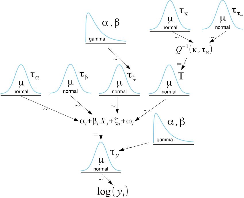
Rehren et al.                                                                                                           A Bayesian Approach for Data-Poor Fisheries

  FIGURE 1 | Chwaka Bay, Zanzibar (Tanzania). The bay comprises large mangrove stands in the south, a fringing reef at the bay opening, and coral patches inside
  the bay. Seagrass meadows are found throughout the bay with dense aggregations toward the central part.

grounds off Marumbi village were demarcated with buoys to                            of the fishing boats that went fishing on the day of sampling.
ensure the protection of Marumbi fishers from dragnet fishing                        The number of fishers sampled per gear and landing site was
(de la Torre-Castro and Lindström, 2010). Despite this locally                       based on the gear and landing site’s relative proportion. The
enforced zone, all gears are deployed throughout the entire bay.                     catch was classified to family, or if possible to species level
For over 20 years, fishers report decreases in their catch rates                     (Bianchi, 1985; Anam and Mostarda, 2012), weighed to the
(de la Torre-Castro and Rönnbäck, 2004; Geere, 2014), which,                         nearest 1 g, and standardized to weight per fisher [weight per
together with the use of small mesh sizes and destructive gears,                     unit of effort (WPUE), kg fisher− 1 ]. The data collection was
has led to a general concern of overfishing in the bay (de la Torre-                 done directly at the beach during landing before the fishers
Castro and Lindström, 2010; de la Torre-Castro et al., 2014).                        sold their catch. Individuals of any size caught during fishing
                                                                                     were landed and used at least for home consumption. The
Data Collection                                                                      number of fishers, boat, gear, and fishing hours and the type
Fisheries data, habitat, and depth information were collected by                     of gear, boat, and propulsion were also collected. We assigned
the first author during the north–east monsoon (January–June)                        each sample to the corresponding lunar cycle (i.e., full moon,
and the south–east monsoon (September–December) season in                            third quarter, new moon, and first quarter) and season (i.e.,
2014. Data collection was carried out on 18 days per month                           north–east monsoon and south–east monsoon). Information
at the main landing sites (i.e., Chwaka village, Uroa village,                       about the fishing location was collected as the name of the
and Marumbi village, Figure 1), covering a minimum of 30%                            fishing ground. In April and December 2014, the main fishing

Frontiers in Marine Science | www.frontiersin.org                                3                                              July 2021 | Volume 8 | Article 621961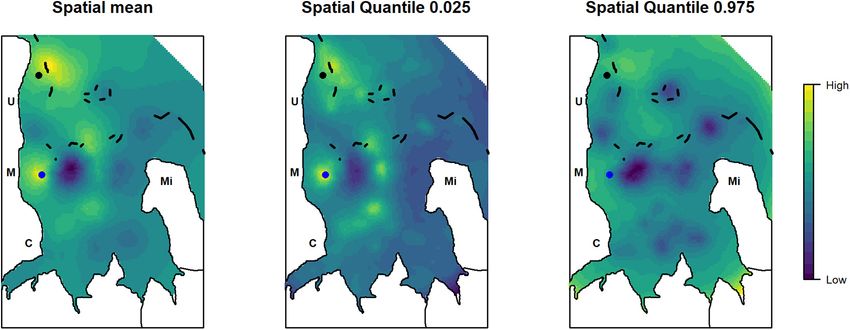
Rehren et al.                                                                                                      A Bayesian Approach for Data-Poor Fisheries

grounds (71%) were mapped together with experienced fishers.                      The relationship between the logarithm of the WPUE and
The depth and seagrass and sand percentage cover were collected               predictors was modeled using a normal distribution (Figure 2).
for 57% of the mapped fishing grounds and on additional non-                  We included an independent and identically distributed random
fished, random locations in the bay. Depth was measured with                  metier effect (Gómez-Rubio, 2020) that accounts for variations
a diving computer and corrected with the tide level records                   in WPUE due to differences in fishing methods and technologies
obtained from the Tanzania Ports Authority.1 The substrate                    (hereafter metier effect). Metiers were assigned to the different
percentage cover was estimated within 2–6 quadrats at each                    samples based on the associated fishing village,4 vessel, gear, and
location. Depth, seagrass, and sand were then interpolated                    propulsion type. We further accounted for spatial autocorrelation
within the spatial extent of the sampling locations using kriging             by including a numeric vector with a mean of 0 and a Matern
techniques. Seagrass nor sand displayed any trend, and thus                   covariance function linking each observation to a spatial location.
ordinary kriging was used with a spherical and exponential                    Thus, our model accounts for independent, region-specific, and
variogram model, respectively. Depth distribution showed a clear              metier-specific noise not explained by the available covariates.
trend, and thus universal kriging with a cubic variogram model                For the parameters involved in the fixed effects, vague Gaussian
was applied to data detrended by a second-order polynomial                    priors with a mean of 0 and a variance of 100 were used, while
trend surface analysis. The interpolation was done using the                  a gamma prior distribution on the precision τ with parameters 1
geoR package (Ribeiro et al., 2020). Shapefiles of coral reef                 and 0.00005 was used for the metier effect. The random spatial
presence–absence were obtained from the Institute of Marine                   effect only depends on two hyperparameters: the range and
Science, Zanzibar. The daily sea-surface temperature of 2014                  the variance of the spatial effect. Penalized complexity priors
was obtained from the GHRSST level 4 data set (0.01◦ × 0.01◦ )                (Fuglstad et al., 2018) were used to describe prior knowledge
downloaded from the OPeNDAP data repository2 using the XML                    on these hyperparameters. We set a prior range of 1 km with a
package (Temple Lang, 2020) implemented in the R software.                    probability of 0.05 for it to be lower and a prior variance of 1.7–2
The temperature was transformed from Kelvin to Celsius, and                   (depending on the species) with a probability of 0.05 for it to be
the annual average was calculated. We used the habitat variables,             higher. We performed a sensitivity analysis of the choice of priors
depth, temperature, lunar cycle, and season as explanatory                    for the spatial effect by testing different priors and verifying that
variables for the distribution of the WPUE of the most dominant               the posterior distributions were consistent and concentrated well
species in the catches (Table 1). We chose the above explanatory              within the support of the priors (Supplementary Figure 1).
variables because they have been identified as key predictors                     Bayesian inference was performed using the Integrated Nested
to determine spatial patterns of marine species (e.g., Beger and              Laplace Approximations (INLA) approach (Rue et al., 2009)
Possingham, 2008; Moore et al., 2009; Roos et al., 2015). The                 with its corresponding package.5 INLA uses the so-called
spatial distribution of the WPUE values was used as a proxy for               Stochastic Partial Differential Equation approach to approximate
the species’ relative abundance.                                              the Gaussian field with the Matern covariance function by a
                                                                              Gaussian Markov random field (Rue et al., 2009).
Statistical Analysis                                                              We selected the most parsimonious model, starting with
All analyses and graphics were performed in R (R Core                         all covariates (except those with VIF values > 3), based on
Team, 20203 ). Prior to the analysis, the explanatory variables               the goodness-of-fit using the deviance information criterion
were standardized (i.e., difference from the mean divided by                  (DIC) (Spiegelhalter et al., 2002) and Watanabe–Akaike
the corresponding standard deviation) (Gelman et al., 2014)                   information criterion (WAIC) (Watanabe, 2010; Supplementary
using the decostand function in the vegan package (Oksanen                    Table 1). The model selection process was automated by
et al., 2019) to better interpret both the direction (positive                using the Bdiclcpomodel_stack function available on GitHub.6
or negative) and magnitude (effect sizes) of the parameter                    We included covariates in the final model if the probability
estimates. We used the variance inflation factor (VIF,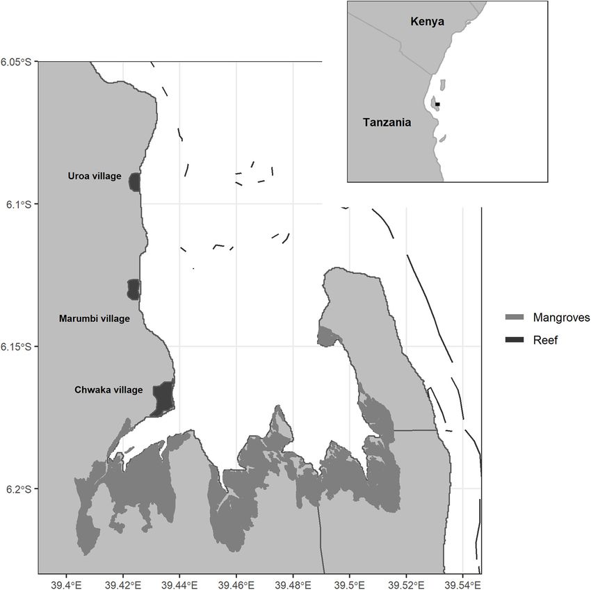
Rehren et al.                                                                                                               A Bayesian Approach for Data-Poor Fisheries

TABLE 1 | Key characteristics of the analyzed target species.

Species                    Family          Habitat association      Depth range            Feeding group      IUCN status     Median size           Main gear
                                                                        [m]                                                    (cm TL)

Siganus sutor             Siganidae          Reef-associated            1–50                  Herbivore       Least concern        19              Trap, dragnet
Lutjanus fulviflamma      Lutjanidae         Reef-associated            3–35                Zoobenthivore     Least concern        18         Dragnet, trap, handline
Lethrinus lentjan        Lethrinidae         Reef-associated            10–90               Zoobenthivore     Least concern        17         Trap, dragnet, handline
Lethrinus mahsena        Lethrinidae         Reef-associated            2–100               Zoobenthivore     Endangered           15         Trap, dragnet, handline
Leptoscarus vaigiensis    Scaridae           Reef-associated            1–15               Herbivore grazer   Least concern        19              Trap, dragnet
Scarus ghobban            Scaridae           Reef-associated            1–90           Herbivore scraper      Least concern        17              Trap, dragnet

While the median size (total length, TL) and main gear were obtained from the present data set, other characteristics were taken from FishBase (Froese and Pauly, 2019).

  FIGURE 2 | Graphical representation of the model. The logarithm of the WPUE (γi ) follows a normal distribution. For the fixed effects parameters, vague Gaussian
  priors with a mean of 0 and a variance of 100 were used. ζi is a Gaussian distributed random metier effect with a mean of 0 and a precision τζ . By default, INLA
  assigns a gamma prior with parameters 1 and 0.00005 to the precision. The random spatial effect (ωi ) is approximated with a Matern covariance function (Q). The
  parameters κ and τω determine the range and the total variance of the spatial effect. The penalized complexity priors of these parameters follow a normal
  distribution. This adaption of a Kruschke style diagram was generated using Bååth (2013) template for LibreOffice.

We further evaluated the final model through residual plots                            of the spatial effect can be seen as a proxy for the species’
(homogeneity of variance, outliers) (Supplementary Figure 2)                           relative abundance.8 The spatial effect maps were then stacked,
and visualizing model predictions. Model assumptions were                              and the posterior distribution of the mean, first, and third
also analyzed by visualizing the predictive integral transform                         quantile was calculated to identify overlapping areas of high
(Supplementary Figure 3), which measures the probability                               relative abundance.
of a new value to be lower than the observed value (Held
et al., 2010). INLA has built-in functions allowing for a                              8
                                                                                        The data and the script for the model construction can be accessed
linear interpolation of the spatial effect within each triangle                        at      https://github.com/Jrehren/Frontiers-2020-Rehren-Supporting-spatial-
into a finer regular grid. The resulting high-resolution map                           management-with-Bayesian-approach

Frontiers in Marine Science | www.frontiersin.org                                  5                                               July 2021 | Volume 8 | Article 621961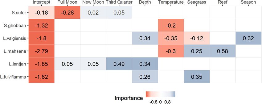
Rehren et al.                                                                                                             A Bayesian Approach for Data-Poor Fisheries

   Figures were created using the ggplot2 package, and maps                             of the environmental variables were found to be important in
were created with the marmap (Pante et al., 2020), mapdata                              the distribution of S. sutor (Figure 3), and only full moon was
(Richard A. Becker and Ray Brownrigg, 2018), mapproj (R by                              selected as a relevant predictor forming a negative relationship
Ray Brownrigg McIlroy et al., 2018), cowplot (Wilke, 2019),                             with abundance. The emperor species showed a strong positive
ggspatial (Dunnington, 2018), rnaturalearth (South, 2017a), and                         relationship with depth (Figure 5), leading to higher relative
rnaturalearthdata (South, 2017b) packages.9                                             abundances around the bay opening close to Uroa and Michamvi
                                                                                        (Figure 4). Reef occurrence was the strongest predictor of
                                                                                        L. mahsena (Figure 3), intensifying the spatial pattern of
RESULTS                                                                                 high relative abundances around the bay opening where the
                                                                                        fringing reef is present. The distribution of L. fulviflamma and
Drivers and Distribution of Target                                                      S. ghobban, contrastingly, showed a spatial pattern of higher
Species                                                                                 relative abundances in the south of the bay (Figure 4). Although
Spatial dependencies and the random metier effect contributed                           the distribution of L. fulviflamma was driven by greater depth,
strongly to the explained variance and hence improved model                             it is even stronger driven by high seagrass cover (Figure 5). It is
performance. The temporal covariates had a relatively strong                            present in dense seagrass meadows in the bay proper and around
effect on species distribution. While the third quarter and                             Chwaka village. The relative abundance of L. vaigiensis indicated
full moon were important covariates for Siganus sutor and                               a slightly negative relationship with seagrass and a strong positive
Lethrinus lentjan (Figure 3), season was only important in                              relationship with depth (Figure 5), leading to a spatial pattern
the distribution of Leptoscarus vaigiensis. This relationship was                       of high values around Uroa toward the bay opening and in the
positive, indicating higher relative abundances for L. vaigiensis                       middle of the bay (Figure 4). The posterior distribution of the
during the south–east monsoon season (Figure 3). The strong                             standard deviation of all spatial effects was relatively high, with
positive relationship between the third quarter moon phase and                          the highest values toward the bay opening and the south of the
the distribution of L. lentjan indicates that this is a relevant                        bay, where the number of observations for the target species
predictor of high WPUE values. Important environmental drivers                          decreases (Figure 4).
were highly variable among species, but the magnitude of their
effects was relatively similar (Figure 3). While depth was an                           Identifying Areas of High Relative
important predictor for the distribution of L. vaigiensis, L. lentjan,
and Lutjanus fulviflamma, temperature was important for Scarus
                                                                                        Abundance
                                                                                        Two main areas of high relative abundance were found by
ghobban, L. vaigiensis, and Lethrinus mahsena (Figure 3). S. sutor
                                                                                        overlaying the mean posterior distribution of the spatial effect
showed a much smoother spatial trend in relative abundance
                                                                                        from all analyzed species: one area in the north of Uroa
across the bay than the other species and had higher numbers
                                                                                        village and one area in front of Marumbi village (Figure 6).
of observations (twofold) (Figure 4). This species is highly
                                                                                        High relative abundances of the target species were also found
dominant in the catches throughout the year and was particularly
                                                                                        close to the patch reefs inside the bay, which is a fishing
caught north of Uroa. The spatial pattern of relative abundance
                                                                                        area frequently visited by fishers even under unfavorable wind
generally shows a clear south to north trend (Figure 4). None
                                                                                        conditions as it is partly protected by the fringing reef. The
9
 Source code for the map can be accessed at https://github.com/MgraziaPennino/          fringing reefs and the deeper outer parts do not seem to create
Create_map_study_area/blob/master/Map_study_area.R                                      areas of particular high relative abundance for the analyzed

    FIGURE 3 | Summary of the selected environmental drivers for each species and the value of the corresponding slope. The legend represents the probability of the
    slope (Importance) to be below (negative, red) or above (positive, blue) zero.

Frontiers in Marine Science | www.frontiersin.org                                   6                                             July 2021 | Volume 8 | Article 621961
Rehren et al. A Bayesian Approach for Data-Poor Fisheries
FIGURE 4 | Posterior mean and standard deviation of the spatial random effect. Letters indicate the position of the villages: C, Chwaka; M, Marumbi; U, Uroa; Mi,
Michamvi. Black lines depict the reef.
target species. The area in front of Marumbi corresponds to The environmental drivers found to be important for
the demarcated dragnet-free zone enforced by the Marumbi species distribution were highly dissimilar between the different
villagers. The area in the north of Uroa lies in the region species. This was very apparent among species of the same
suggested by the fishers as a no-take zone during the participatory family: for the two emperor species, relevant selected predictors
workshop conducted in 2016. Both also remain areas of higher were opposite and for the two parrotfish, the only common
relative abundance in the posterior distribution of the upper and environmental driver was temperature. Contrastingly, season was
lower quantiles. only an important driver of the distribution of L. vaigiensis.
The weak influence of seasons on fish density is a general
pattern observed in Chwaka Bay’s mangrove creeks (Mwandya
DISCUSSION et al., 2010) and the seagrass meadows close to Chwaka
and Marumbi village (Lugendo et al., 2007). Only the heavy
Main Drivers of Species Distribution rain season from April to May has been shown by Lugendo
Understanding species distribution is a key aspect in setting et al. (2007) to induce significant changes in environmental
successful spatio-temporal management plans (Franklin, 2009; factors and fish density inside the mangrove creeks of Chwaka
Lawler et al., 2011; Guisan et al., 2013). The results from this Bay. This suggests relatively stable annual catches of the
study provide information on important distribution drivers of other target species, representing a significant part of trap
the WIO’s key target species and commonalities among them. and dragnet catch (Rehren et al., 2018a). Reduced temporal
Frontiers in Marine Science | www.frontiersin.org 7 July 2021 | Volume 8 | Article 621961Rehren et al. A Bayesian Approach for Data-Poor Fisheries FIGURE 5 | Functional response of the weight per unit of effort of each species to their main environmental drivers. Solid lines and shaded regions are the mean and 95% credibility intervals, respectively. NEMS stands for North–East Monsoon Season and SEMS for South–East Monsoon Season. FIGURE 6 | Posterior distribution of the mean, first, and third quantile of the combined spatial effect of the analyzed species to identify areas of overlapping high relative abundance. The dots represent a dragnet free zone (blue) enforced by the Marumbi fishers and the area proposed for the implementation of a no-take zone during the participatory workshop in 2016 (black). Letters indicate the position of the villages: C, Chwaka; M, Marumbi; U, Uroa; Mi, Michamvi. Black lines depict the reef. fluctuations in catches and the protection from wave energy The full moon lunar phase was the only relevant predictor through the fringing reef makes the bay a vital fishing ground for S. sutor. This species is of high importance to Chwaka Bay’s that decreases the vulnerability of the fishing community. fishery since it dominates the main gears, and its annual yield Attempts to reallocate fishing efforts to offshore areas, which strongly exceeds all other target species (Rehren et al., 2018b). has been part of past management actions (Gustavsson S. sutor grazes over algae beds, and juveniles mainly use seagrass et al., 2014), need to compensate for a potential increase in meadows as nurseries (Dorenbosch et al., 2005; Lugendo et al., income uncertainty. 2005; Kimirei et al., 2011). Larger individuals are usually found Frontiers in Marine Science | www.frontiersin.org 8 July 2021 | Volume 8 | Article 621961
Rehren et al.                                                                                            A Bayesian Approach for Data-Poor Fisheries

around reefs and are associated with deeper depths (Kimirei                abundance. Although these results seem counterintuitive,
et al., 2011). Accordingly, the spatial distribution of S. sutor           Gullström et al. (2011) also found a negative relationship
shows a clear increasing trend in relative abundance toward the            between shoot density and the variability of juvenile and adult
bay opening and, thus, deeper areas. S. sutor, unlike the more             density of L. vaigiensis. Fish assemblages in coral reef and
sedentary emperor species, is a relatively mobile species with a           seagrass habitats in Kenya likewise showed a decrease in overall
home range of about 900 m (Ebrahim et al., 2020a). This might              density with increasing seagrass density (Chirico et al., 2017).
explain its smoother distribution and the lack of patches in the           The authors argued that this relationship possibly arises due
spatial random effect compared to the other species.                       to the reduced movement ability of fish in very dense and
    Our analysis indicates that seagrass plays an important                relatively short seagrass beds. Stronger environmental drivers of
role in the distribution of the emperor species L. mahsena,                L. vaigiensis were depth and temperature in our models, which
the parrotfish L. vaigiensis, and the snapper L. fulviflamma.              probably explains its high relative abundance around the north
L. fulviflamma uses seagrass meadows and particularly mangrove             of Uroa and in the middle of the bay. Gullström et al. (2011)
swamps as nursery areas (Lugendo et al., 2005; Kimirei et al.,             also found temperature to be a driver for the abundance of
2011), explaining the higher relative abundances found in the              L. vaigiensis within different seagrass meadows in Chwaka Bay,
south of the bay. During the workshop in 2016 with 30                      but not depth. The authors, however, mainly studied seagrass
participants, fishers reported that L. fulviflamma used to occur           meadows along the shore, which does not represent the full
in higher quantities in the bay and that the species seemed                range of depth in the bay, possibly explaining the differences in
to have moved toward deeper waters due to an increase in                   our model results.
water temperatures (Rehren, 2017). While our model indicates a
positive relationship of L. fulviflamma distribution with depth,           Potential Areas for Conservation
temperature was not selected as a relevant predictor. Along                Spatio-temporal management is a key strategy to help mitigate
this line, other studies conducted in Tanzania mainland found              conflicts among fishers and protect essential habitats and target
that depth best explained the size-frequency distribution of               species, without entirely depriving fishers of their economic basis
L. fulviflamma among habitats (Kimirei et al., 2015) with                  (Rassweiler et al., 2012; Kerwath et al., 2013; Sale et al., 2014;
adult specimens found on deeper reefs (Kimirei et al., 2011).              Di Franco et al., 2016; Sala et al., 2021). In the WIO region,
Temperature, however, was selected as the main driver for                  the implementation of conservation areas has been a prime
three of the other analyzed species, including S. ghobban, and             management tool to reduce anthropogenic pressures (IUCN.,
overall species density is also negatively related to temperature          2004). In this study, we identified areas of high relative abundance
in mangrove and mud/sand habitats of the bay (Lugendo et al.,              of six key target species of the region to provide information for
2007). Dorenbosch et al. (2005) found high juvenile densities              the prioritization of such conservation areas.
(>70%) and intermediate adult densities (30–70%) of S. ghobban                 The identified overlapping areas of high relative abundance
in seagrass meadows, likely explaining its high relative abundance         are in the north of Uroa, close to reef areas, and in front of
found in the central bay and in the south of the bay where                 Marumbi village, dominated by seagrass meadows. Furthermore,
seagrass meadows occur.                                                    areas close to the patch reefs surrounded by seagrass meadows
    Lethrinus mahsena, also found to be driven by seagrass cover,          inside the bay also showed higher relative abundances. Both
is a generalist occurring in all habitats of the bay (Dorenbosch           emperor species, the rabbitfish S. sutor, and the parrotfish
et al., 2005) and is particularly associated with coral patches and        L. vaigiensis would benefit from the closure of fishing in the
fringing reefs adjacent to seagrass beds (Gell and Whittington,            selected areas. Except for Uroa, the identified areas do not
2002; Locham et al., 2010). This observation also matches our              occur on the proper fringing reef that runs along the bay
findings that the most important driver of its abundance was               opening. Although we use the analyzed WPUE values as a
reef, followed by temperature and seagrass. Accordingly, areas of          proxy for relative abundance, the absence of high relative
high relative abundance of L. mahsena were found around coral              abundances on the fringing reef is likely a mere reflection
patches inside the bay, which are surrounded by large seagrass             of the distribution of effort: the exposure and deeper depths
meadows and at the fringing reef in the north of Uroa. High                at the fringing reef make it harder to fish with the main
relative abundances were also found in front of Marumbi village,           fishing methods. However, the WPUE distribution pattern
a fishing ground dominated by dense seagrass beds.                         indicates that proper reef areas with high coral cover are not
    Little information was available for the other emperor species,        necessarily areas with the highest fishing pressure in small-
L. lentjan, which occurs in all habitats of the bay (Lugendo et al.,       scale fisheries of the WIO region and that non-reef areas in
2005). The adult part of the population mostly occurs around               Chwaka Bay may be as suitable for spatio-temporal management
the reef areas (Dorenbosch et al., 2005). Depth was the only               plans. These findings match the observation from de la Torre-
environmental predictor selected in our model and probably                 Castro et al. (2014) that seagrass meadows, and not reefs,
explains the higher relative abundances in the north of Uroa and           are the fishing grounds with the highest community benefits
the area around Michamvi.                                                  for the fishers of Chwaka village. In the WIO region, spatial
    While L. vaigiensis mainly occurs in seagrass beds                     management plans are often implemented to protect a specific
(Dorenbosch et al., 2005; Lugendo et al., 2005) and feeds                  habitat (Turpie et al., 2000; Wells et al., 2007; Rocliffe et al.,
on seagrass plants (Gullström et al., 2011), our results showed a          2014), which has led to the disproportionate representation of
slight negative relationship between seagrass cover and relative           coral reefs in marine conservation areas (Wells et al., 2007;

Frontiers in Marine Science | www.frontiersin.org                      9                                        July 2021 | Volume 8 | Article 621961
Rehren et al. A Bayesian Approach for Data-Poor Fisheries
de la Torre-Castro et al., 2014; Chirico et al., 2017). The need to this data, such as spatial dependencies and the fisher effect,
include seagrass meadows into fisheries management efforts has through their direct incorporation in the model formulation
not only been highlighted for the bay (de la Torre-Castro et al., (Banerjee et al., 2004; Pennino et al., 2019).
2014) but globally (Unsworth et al., 2019). Our analysis shows that a large part of the variance
Conservation areas are often selected without incorporating was explained by the random effect terms highlighting the
fisher’s behavior in the implementation of spatio-temporal importance of spatial dependencies and effects stemming from
management plans, which has led to weak compliance the use of different gears, boats, and propulsions. The latter
(McClanahan et al., 2006; Rosendo et al., 2011) and reduced effect is very high, suggesting that Chwaka Bay’s fisheries might
benefits for fishing communities (Benjaminsen and Bryceson, be better managed based on fishing units. This requires flexible
2012). For instance, Marine parks in Kenya have been established and adaptive management approaches tailored around the
with little consultation of fishing communities, and in Tanzania, dynamic behavior of fishers in space, time, and fishing methods.
examples of opposing the enforcement of existing conservation A clear benefit of Bayesian models in data-poor situations is
areas exist (Wells et al., 2007). This is surprising as fishers the provision of uncertainty associated with the data and the
have shown to possess strong ecological knowledge about their parameter estimates (Banerjee et al., 2004; Fonseca et al., 2017).
target stocks (Silvano and Valbo-Jørgensen, 2008). Lopes et al. This is particularly important when the stakes are high, as is
(2018) have shown that fisher’s knowledge can even be reliable the case in small-scale fishing communities. Our analysis shows
enough for predicting species occurrence. These observations that the uncertainties associated with our results are relatively
are also reflected in our analysis: the two areas of high relative high, particularly for the areas in the south and the north of the
abundance correspond to the areas that: (1) have been prioritized bay. A central issue associated with fisheries-dependent data is
by fishers for the dragnet free zone in front of Marumbi village that fishers have prior knowledge of the probability of catching
in 2001 (de la Torre-Castro and Lindström, 2010); and (2) have their target species at a given location leading to sampling bias.
been proposed as a potential no-take zone in the workshop of Furthermore, in our case study, greater depths and the presence
2016 (Rehren, 2017). This study has been conducted to support of hard corals make fishing harder for dragnet fisher, lowering the
local spatio-temporal management actions with quantitative number of observations at the fringing reef. Our approach does
information. In a series of upcoming participatory workshops, not account for such sampling bias in the data, which might have
the relative abundance maps with their associated uncertainties influenced the identification of the high relative abundance areas.
will be used to effectively visualize and convey our key findings to Another limitation is the difficulty in obtaining a precise geo-
the local stakeholders. With these workshops, we aim to combine localization of the catch in tropical, small-scale fisheries because
short-term fisheries dependent data and fishers’ knowledge of the large number of vessels, their dynamic behavior, and the
to synthesize the most relevant information about the spatial lack of technical equipment. Usually, the spatial location of the
dynamics of Chwaka Bay’s fisheries and target resources and to catch is associated with a fishing ground name and mapped
prioritize spatial management actions. subsequently, or the fishing ground location is identified on a
map by the fisher. These procedures reduce the spatial precision
of the catch and can mislead inference. The observation that
Potential and Limitations of the our model selects the same area for conservation as fishers
Approach did during the participatory workshop in 2016 (Rehren, 2017)
In many small-scale fisheries, dependence on resources for increases the confidence in our model results. It must be noted
livelihood and protein supply is high, making their sustainable that these action plans were formulated and discussed with a
management particularly important (Belhabib et al., 2015; Teh limited number of fishers. A comparison of our results with
and Pauly, 2018; Loring et al., 2019; Salas et al., 2019). information from ecological studies about the habitat preference
Appropriate management plans are, however, impeded by the and ecology of four of the analyzed species also suggests that
notorious lack of data (Salas et al., 2007; Salayo et al., 2008; our approach predicts the distribution of the analyzed species
Samoilys et al., 2015). Fisheries independent surveys are often reasonably well. For the remaining two species (i.e., S. ghobban,
cost-intensive and visual census data collected around Zanzibar L. lentjan), not enough information was found to evaluate our
are spatially limited and only represent a temporal snapshot models properly. For S. sutor, it is likely that we missed to
(Rehren et al., 2020). Fisheries catch information, on the other include the distribution of macroalgae in the bay as a predictor
hand, is collected throughout the WIO region at a subset of variable because S. sutor grazes on epibenthic algae and feeds on
landing sites (UNEP-Nairobi Convention and WIOMSA, 2015) macroalgae thalli (Ebrahim et al., 2020b). But it is also possible
and thus becomes the most cost-effective and accessible source that the spatial change in environmental or habitat variables in
of information when evaluating the spatio-temporal dynamics the bay is not strong enough to significantly affect S. sutor’s
of target resources. Suppose that fishers’ catches represent distribution because the area is relatively small and S. sutor’s
thousands of sampling observations (García-Quijano, 2007) and mobility is relatively high. Salinity and primary productivity
those fishers use multiple gears catching a multitude of species. are other predictors that have been identified to drive species
In that case, it can be argued that fisheries catches as a whole distribution (Roos et al., 2015; Gonzáles-Andrés et al., 2016; Coll
might better reflect species relative abundance than spatially et al., 2019). Studies from the bay, however, suggest that salinity
and temporally limited visual census data. Bayesian hierarchical is not a driver of fish density (Lugendo et al., 2007) and that
modeling approaches can better handle problems associated with habitat variables generally are more important predictors for fish
Frontiers in Marine Science | www.frontiersin.org 10 July 2021 | Volume 8 | Article 621961Rehren et al. A Bayesian Approach for Data-Poor Fisheries
assemblages and abundance (Gullström et al., 2008; Mwandya ecological principles of complementarity, representativeness, and
et al., 2010). connectivity (Ban et al., 2011).
Information on environmental drivers at a high-resolution
scale is often lacking, making it difficult to model the distribution
of resources in small fishing areas such as Chwaka Bay. DATA AVAILABILITY STATEMENT
We used data collected by the first author about depth and
habitat variables and interpolated them to get an estimate The datasets presented in this study can be found in
at all fishing grounds. Thereby, we did not consider the online repositories. The names of the repository/repositories
uncertainty associated with the covariate estimations, which and accession number(s) can be found below: https://
can cause erroneous inference and a biased estimate of the github.com/Jrehren/Frontiers-2020-Rehren-Supporting-spatial-
covariate effect (Martínez-Minaya et al., 2018). Consequently, management-with-Bayesian-approach.git.
we compared models with and without the interpolated data:
while some species had similar spatial random effect maps,
for other species using the non-interpolated data resulted AUTHOR CONTRIBUTIONS
in peaks or throughs at missing locations (Supplementary
Figure 4). In other words, including only a subset of the MP, MC, and JR conceived and designed the research. NJ and JR
data would have resulted in misidentifying areas of high designed the data collection. MP and JR performed the analysis.
relative abundance. Ideally, information on environmental CM provided data for the analysis and the maps. MP, MC, NJ,
covariates should be available at all fishing grounds to avoid CM, and JR wrote the manuscript. All authors contributed to the
potential misalignment. article and approved the submitted version.
Areas prioritized by the fishing community or the approach
used here may not be sufficient to achieve ecological objectives.
The structural complexity of seagrass meadows in the bay, for FUNDING
instance, is an important factor that can drive fish abundance
(Gullström et al., 2008) and habitats often function together This project was funded by the German Research Foundation
with surrounding habitats determining fish composition through (DFG) within a research fellowship program (RE 4358/1-1). The
seascape structure (Berkström et al., 2012). Furthermore, the data used in the analysis was collected in 2014 within a program
areas prioritized by the Chwaka Bay fishers are relatively (SUTAS) funded by the Leibniz Gemeinschaft. MC acknowledges
small, while large marine protected areas are associated with the ‘Severo Ochoa Centre of Excellence’ accreditation (CEX2019-
higher success, particularly when protecting highly mobile 000928-S) to the Institute of Marine Science (ICM-CSIC).
species (Claudet et al., 2008; Vandeperre et al., 2011; Edgar
et al., 2014; White et al., 2017). But it has also been
shown that small community-based marine protected areas SUPPLEMENTARY MATERIAL
established in coral reef developing nations may nonetheless
be highly successful (Ban et al., 2011; Chirico et al., 2017). The Supplementary Material for this article can be found
In the long-term such conservation efforts need to be online at: https://www.frontiersin.org/articles/10.3389/fmars.
scaled up to regional or national levels to achieve the 2021.621961/full#supplementary-material
REFERENCES Bene, C., Macfadyen, G., and Alisson, E. H. (2007). Increasing the Contribution of
Small-Scale Fisheries to Poverty Alleviation and Food Security. Rome: FAO.
Anam, R., and Mostarda, E. (2012). Field Identification Guide to the Living Marine Benjaminsen, T. A., and Bryceson, I. (2012). Conservation, green /blue grabbing
Resources of Kenya. FAO Species Identification Guide for Fishery Purposes. Rome: and accumulation by dispossession in Tanzania. J. Peasant Stud. 39, 37–41.
FAO. doi: 10.1080/03066150.2012.667405
Bååth (2013). Available online at: http://www.sumsar.net/blog/2013/10/diy- Berkström, C., Gullström, M., Lindborg, R., Mwandya, A. W., Yahya, S. A. S.,
kruschke-style-diagrams/ (accessed January 10, 2021). Kautsky, N., et al. (2012). Exploring ’knowns’ and ’unknowns’ in tropical
Ban, N. C., Adams, V. M., Almany, G. R., Ban, S., Cinner, J. E., McCook, L. J., seascape connectivity with insights from East African coral reefs. Estuar. Coast.
et al. (2011). Designing, implementing and managing marine protected areas: Shelf Sci. 107, 1–21. doi: 10.1016/j.ecss.2012.03.020
emerging trends and opportunities for coral reef nations. J. Exp. Mar. Biol. Ecol. Bianchi, G. (1985). FAO Species Identification Sheets for Fishery Purposes. Field
408, 21–31. doi: 10.1016/j.jembe.2011.07.023 Guide to the Commercial and Marine Brackish-Water Species of Tanzania.
Banerjee, S., Carlin, B. P., and Gelfand, A. E. (2004). Hierarchical Modeling and Project No. TCP/URT/4406. Rome: FAO.
Analysis for Spatial Data. Boca Raton, FL: Chapman and Hall. CBD, (2010). Strategic Plan for Biodiversity 2011-2020 and the Aichi Targets. Report
Beger, M., and Possingham, H. P. (2008). Environmental factors that influence of the Tenth Meeting of the Conference of the Parties to the Convention on
the distribution of coral reef fishes: modeling occurrence data for broad-scale Biological Diversity. Nagoya: CBD.
conservation and management. Mar. Ecol. Prog. Ser. 361, 1–13. doi: 10.3354/ Chirico, A. A. D., McClanahan, T. R., and Eklöf, J. S. (2017). Community- and
meps07481 government-managed marine protected areas increase fish size, biomass and
Belhabib, D., Sumaila, U. R., and Pauly, D. (2015). Feeding the poor: contribution potential value. PLoS One 12:e0182342. doi: 10.1371/journal.pone.0182342
of West African fisheries toemployment and food security. Ocean and Coast. Chuenpagdee, R. (ed.) (2011). World Small Scale Fisheries Contemporary Visions.
Manag. 111, 72–81. doi: 10.1016/j.ocecoaman.2015.04.010 Delft: Eburon Academic Publishers.
Frontiers in Marine Science | www.frontiersin.org 11 July 2021 | Volume 8 | Article 621961Rehren et al. A Bayesian Approach for Data-Poor Fisheries
Claudet, J., Osenberg, C. W., Benedetti-Cecchi, L., Domenici, P., García- García-Quijano, C. G. (2007). Assemblages : bridging between scientific and
Charton, J. A., Pérez-Ruzafa, Á, et al. (2008). Marine reserves: size and local ecological knowledge in Southeastern Puerto Rico. Am. Anthropol. 109,
age do matter. Ecol. Lett. 11, 481–489. doi: 10.1111/j.1461-0248.2008. 529–536. doi: 10.1525/AA.2007.109.3.529.530
01166.x Geere, D. (2014). Adaption to Climate-Related Changes in Seagrass Ecosystems in
Coll, M., Pennino, M. G., Steenbeek, J., Solé, J., and Bellido, J. M. (2019). Predicting Chwaka Bay (Zanzibar). Göteborg: University of Göteborg.
marine species distributions: complementarity of food web and Bayesian Gell, F. R., and Whittington, M. W. (2002). Diversity of fishes in seagrass beds in the
hierarchical modelling approaches. Ecol. Model. 405, 86–101. Quirimba Archipelago, northern Mozambique. Mar. Freshw. Res. 53, 115–121.
Daw, T. M. (2008). Spatial distribution of effort by artisanal fishers: exploring doi: 10.1071/MF01125
economic factors affecting the lobster fisheries of the Corn Islands, Nicaragua. Gelman, A., Carlin, J., Stern, H., and Rubin, D. (2014). Bayesian Data Analysis, Vol.
Fish. Res. 90, 17–25. doi: 10.1016/j.fishres.2007.09.027 2. Boca Raton, FL: Chapman & Hall.
de la Torre-Castro, M., Di Carlo, G., and Jiddawi, N. S. (2014). Seagrass Gómez-Rubio, V. (2020). Bayesian Inference with INLA. London: Chapman and
importance for a small-scale fishery in the tropics: the need for seascape Hall.
management. Mar. Pollut. Bull. 83, 398–407. doi: 10.1016/j.marpolbul.2014. Gonzáles-Andrés, C., Lopes, P. F. M., Cortés, J., Sánchez-Lizaso, J. L., and Pennino,
03.034 M. G. (2016). Abundance and distribution patterns of Thunnus albacares in Isla
de la Torre-Castro, M., and Lindström, L. (2010). Fishing institutions: addressing del Coco National Park through predictive habitat suitability models. PLoS One
regulative, normative and cultural-cognitive elements to enhance fisheries 11:e0168212. doi: 10.1371/journal.pone.0168212
management. Mar. Policy 34, 77–84. doi: 10.1016/j.marpol.2009.04.012 Guisan, A., Reid, T., Baumgartner, J. B., Naujokaitis-Lewis, I., Sutcliffe, P. R.,
de la Torre-Castro, M., and Rönnbäck, P. (2004). Links between humans and Tulloch, A. I. T., et al. (2013). Predicting species distributions for conservation
seagrasses – an example from tropical East Africa. Ocean Coast. Manag. 47, decisions. Ecology Letters 16, 1424–1435. doi: 10.1111/ele.12189
361–387. doi: 10.1016/j.ocecoaman.2004.07.005 Gullström, M., Berkström, C., Öhman, M. C., Bodin, M., and Dahlberg, M. (2011).
De Santo, E. M. (2013). Missing marine protected area (MPA) targets: how the push Scale-dependent patterns of variability of a grazing parrotfish (Leptoscarus
for quantity over quality undermines sustainability and social justice. J. Environ. vaigiensis) in a tropical seagrass-dominated seascape. Mar. Biol. 158, 1483–
Manag. 124, 137–146. doi: 10.1016/j.jenvman.2013.01.033 1495. doi: 10.1007/s00227-011-1665-z
Department of Fisheries Development. (2016). Marine Fisheries Frame Survey Gullström, M., Bodin, M., Nilsson, P. G., and Öhman, M. C. (2008). Seagrass
2016, Zanzibar. Zanzibar: Ministry of Agriculture, Natural Resources, structural complexity and landscape configuration as determinants of tropical
Livestock; Fisheries Zanzibar. SWIOFish Project/World Bank. Department of fish assemblage composition. Mar. Ecol. Prog. Ser. 363, 241–255. doi: 10.3354/
Fisheries Development. meps07427
Di Franco, A., Thiriet, P., Di Carlo, G., Dimitriadis, C., Francour, P., Gutiérrez, Gullström, M., Dorenbosch, M., Lugendo, B. R., Mwandya, A. W., Mgaya, Y. D.,
N. L., et al. (2016). Five key attributes can increase marine protected areas and Berkström, C. (2012). “Biological connectivity and nursery function of
performance for small-scale fisheries management. Sci. Rep. 6, 1–9. doi: 10. shallow-water habitats in Chwaka Bay,” in People, Nature and Research in
1038/srep38135 Chwaka Bay, Zanzibar, Tanzania, eds M. de la Torre-Castro, and T. J. Lyimo
Dorenbosch, M., Grol, M. G. G., Christianen, M. J. A., Nagelkerken, I., and Van Der (Zanzibar Town: WIOMSA), 175–192.
Velde, G. (2005). Indo-Pacific seagrass beds and mangroves contribute to fish Gullström, M., Lunden, B., Bodin, M., Kangwe, J., Öhman, M. C., Mtolera, M. S. P.,
density and diversity on adjacent coral reefs. Mar. Ecol. Prog. Ser. 302, 63–76. et al. (2006). Assessment of changes in the seagrass-dominated submerged
doi: 10.3354/meps302063 vegetation of tropical Chwaka Bay (Zanzibar) using satellite remote sensing.
Dunnington, D. (2018). Ggspatial: Spatial Data Framework for ggplot2. Available Estuar. Coast. Shelf Sci. 67, 399–408. doi: 10.1016/j.ecss.2005.11.020
online at: https://CRAN.R-project.org/package=ggspatial (accessed January 4, Gustavsson, M., Lindström, L., Jiddawi, N. S., and de la Torre-Castro, M. (2014).
2021). Procedural and distributive justice in a community-based managed marine
Ebrahim, A., Bijoux, J. P., Mumby, P. J., and Tibbetts, I. R. (2020a). The protected area in Zanzibar, Tanzania. Mar. Policy 46, 91–100. doi: 10.1016/j.
commercially important shoemaker spinefoot, Siganus sutor, connects coral marpol.2014.01.005
reefs to neighbouring seagrass meadows. J. Fish Biol. 96, 1034–1044. doi: 10. Held, L., Schrödle, B., and Rue, H. (2010). “Posterior and cross-validatory
1111/jfb.14297 predictive checks: a comparison of MCMC and INLA,” in Statistical Modelling
Ebrahim, A., Martin, T. S. H., Mumby, P. J., Olds, A. D., and Tibbetts, I. R. and Regression Structures: Festschrift in Honour of Ludwig Fahrmeir, eds T.
(2020b). Differences in diet and foraging behaviour of commercially important Kneib, and G. Tutz (Heidelberg: Physica-Verlag HD), 91–110. doi: 10.1007/
rabbitfish species on coral reefs in the Indian Ocean. Coral Reefs 39, 977–988. 978-3-7908-2413-1_6
doi: 10.1007/s00338-020-01918-6 IUCN. (2004). Managing Marine Protected Areas: A Toolkit for the Western Indian
Edgar, G. J., Stuart-Smith, R. D., Willis, T. J., Kininmonth, S., Baker, S. C., Banks, Ocean. Nairobi: IUCN Eastern African Regional Programme.
S., et al. (2014). Global conservation outcomes depend on marine protected Jiddawi, N., and Lindström, L. (2012). “Physical characteristics, socio-economic
areas with five key features. Nature 506, 216–220. doi: 10.1038/nature1 setting and coastal livelihoods in Chwaka Bay,” in People, Nature and Research
3022 in Chwaka Bay, Zanzibar, Tanzania, eds M. de la Torre-Castro, and T. J. Lyimo
FAO. (2015). Voluntary Guidelines for Securing Sustainable Small-Scale Fisheries. (Zanzibar Town: WIOMSA), 23–40.
Rome: Food; Agriculture Organisation of the United Nations. Jiddawi, N. S. (2012). “Artisanal fisheries and other marine resources in Chwaka
FAO. (2018). Voluntary Guidelines for Securing Sustainable Small-Scale Fisheries Bay,” in People, Nature, and Research in Chwaka Bay, Zanzibar, Tanzania, eds
in the Context of Food Security and Poverty Eradication. Available online at: M. de la Torre-Castro, and T. J. Lyimo (Zanzibar Town: WIOMSA), 193–212.
http://www.fao.org/docrep/field/003/ab825f/AB825F00.htm{#}TOC (accessed Jiddawi, N. S., and Ohman, M. C. (2002). Marine fisheries in Tanzania. Ambio 31,
May 31, 2021). 518–527.
Fonseca, V. P., Pennino, M. G., de Nóbrega, M. F., Oliveira, J. E. L., Kerwath, S. E., Winker, H., Götz, A., and Attwood, C. G. (2013). Marine protected
and de Figueiredo Mendes, L. (2017). Identifying fish diversity hot- area improves yield without disadvantaging fishers. Nat. Commun. 4, 1–6. doi:
spots in data-poor situations. Mar. Environ. Res. 129, 365–373. doi: 10.1038/ncomms3347
10.1016/j.marenvres.2017.06.017 Kimirei, I. A., Nagelkerken, I., Griffioen, B., Wagner, C., and Mgaya, Y. D.
Franklin, J. (ed.) (2009). Mapping Species Distributions: Spatial Inference and (2011). Ontogenetic habitat use by mangrove/seagrass-associated coral reef
Prediction. Cambridge: CambridgeUniversity press. fishes shows flexibility in time and space. Estuar. Coast. Shelf Sci. 92, 47–58.
Froese, R., and Pauly, D. (2019). FishBase. Available online at: http://www.fishbase. doi: 10.1016/j.ecss.2010.12.016
org (accessed February 8, 2020) Kimirei, I. A., Nagelkerken, I., Slooter, N., Gonzalez, E. T., Huijbers, C. M., Mgaya,
Fuglstad, G. A., Simpson, D., Lindgren, F., and Rue, H. (2018). Constructing priors Y. D., et al. (2015). Demography of fish populations reveals new challenges
that penalize the complexity of Gaussian random fields. J. Am. Stat. Assoc. 114, in appraising juvenile habitat values. Mar. Ecol. Prog. Ser. 518, 225–237. doi:
445–452. doi: 10.1080/01621459.2017.1415907 10.3354/meps11059
Frontiers in Marine Science | www.frontiersin.org 12 July 2021 | Volume 8 | Article 621961You can also read