Soil total phosphorus and nitrogen explain vegetation community composition in a northern forest ecosystem near a phosphate massif - Biogeosciences
←
→
Page content transcription
If your browser does not render page correctly, please read the page content below
Biogeosciences, 17, 1535–1556, 2020
https://doi.org/10.5194/bg-17-1535-2020
© Author(s) 2020. This work is distributed under
the Creative Commons Attribution 4.0 License.

Soil total phosphorus and nitrogen explain vegetation community
composition in a northern forest ecosystem near a phosphate massif
Laura Matkala1 , Maija Salemaa2 , and Jaana Bäck1
1 Institute
          for Atmospheric and Earth System Research/Forest Sciences, Faculty of Agriculture
and Forestry, University of Helsinki, P.O. Box 27, 00014 Helsinki, Finland
2 Natural Resources Institute Finland (Luke), Latokartanonkaari 9, 00790 Helsinki, Finland

Correspondence: Laura Matkala (laura.matkala@helsinki.fi)

Received: 25 March 2019 – Discussion started: 13 May 2019
Revised: 22 January 2020 – Accepted: 22 February 2020 – Published: 26 March 2020

Abstract. The relationship of the community composition            1   Introduction
of forest vegetation and soil nutrients were studied near the
Sokli phosphate ore deposit in northern Finland. Simulta-
neously, the effects of the dominant species and the age of        Climate and availability of soil nutrients are important fac-
trees, rock parent material and soil layer on these nutrients      tors controlling the species composition of tree stand and un-
were examined. For this purpose, 16 study plots were es-           derstorey vegetation in boreal forests (Cajander, 1909, 1949;
tablished at different distances from the phosphate ore along      Kuusipalo, 1985; Økland and Eilertsen, 1996). High-latitude
four transects. Phosphate mining may take place in Sokli in        forest ecosystems are characteristically cold, have a short
the future, and the vegetation surveys and soil sampling con-      growing season and are nutrient poor. Organic matter de-
ducted at the plots can be used as a baseline status for fol-      composition and nutrient release are usually slow in cold
lowing the possible changes that the mining may cause in the       climates (Hobbie et al., 2002). The edaphic conditions are
surrounding ecosystem. The total phosphorus (P) and nitro-         reflected in the growth and chemical composition of plant
gen (N) contents of the soil humus layer were positively re-       species, as well as in species composition of vegetation (Vin-
lated with species number and abundance of the understorey         ton and Burke, 1995; Salemaa et al., 2008). In addition, tree
vegetation, and the correlation was slightly higher with P         cover affects the species composition and abundance in the
than N. This is interesting, as N usually has the most im-         understorey by shading (Verheven et al., 2012; Tonteri et al.,
portant growth-limiting role in boreal ecosystems. The spa-        2016) and regulating nutrient input in throughfall precipita-
tial variation in the content of soil elements was high both       tion (Salemaa et al., 2019) and litterfall (Ukonmaanaho et al.,
between and within plots, emphasizing the heterogeneity of         2008).
the soil. Dominant tree species and the soil layer were the           Nitrogen (N) and phosphorus (P) are generally the main
most important environmental variables affecting soil nutri-       growth-limiting nutrients for plants (Koerselman and Meule-
ent content. High contents of P in the humus layer (maxi-          man, 1996). Boreal forests are mostly N limited (Tamm,
mum 2.60 g kg−1 ) were measured from the birch-dominated           1991), and fertilization with N usually speeds up forest
plots. As the P contents of birch leaves and leaf litter were      growth (Saarsalmi and Mälkönen, 2001). Nitrogen is bound
also rather high (2.58 and 1.28 g kg−1 , respectively), this may   in organic material, and only a little is directly available for
imply that the leaf litter of birch forms an important source      plants as inorganic ammonium (NH4+ ) and nitrate (NO3− )
of P for the soil. The possible mining effects, together with      (Marschner, 1995) or as organic forms like amino acids
climate change, can have an influence on the release of nutri-     (Näsholm et al., 2008, and references within). Phosphorus
ents to plants, which may lead to alterations in the vegetation    deficiency occurs in temperate and tropical forest ecosys-
community composition in the study region.                         tems, but P is rarely a limiting factor in boreal forests on
                                                                   mineral soil (Augusto et al., 2017). However, P can be growth
                                                                   limiting on boreal peatlands (Moilanen et al., 2010; Brække

Published by Copernicus Publications on behalf of the European Geosciences Union.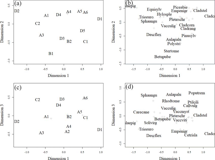
1536                     L. Matkala et al.: Soil total phosphorus and nitrogen explain vegetation community composition

and Salih, 2002). The ratio of soil N to soil P is significant        We hypothesize that there are positive relationships be-
for forest growth on a global scale (Augusto et al., 2017).         tween the following factors:
Hedwall et al. (2017) found that the species richness of vas-
                                                                        a. N and P contents of the soil humus layer and the abun-
cular plants in a temperate forest doubled with combined NP
                                                                           dance and species composition of the understory vege-
fertilization in southern Sweden but not when either of the
                                                                           tation,
nutrients was added alone. This positive effect was strongest
in grass species. In boreal N-limited forests, the number of            b. N and P contents in the topmost soil layers and the N
vascular plant species (grasses and forbs) increased with in-              and P contents of needle and leaf biomass,
creasing N concentration of the organic layer (Salemaa et al.,
2008). Hofmeister et al. (2009) noticed that in a temperate             c. N and P contents in the topmost soil layers and the oc-
forest the species richness of the herb layer was higher in                currence of birch trees in the research plots.
P-rich than P-poor soils but only if strong N limitation oc-
curred simultaneously in the P-rich soils. However, in many         2     Material and methods
regions where humans have enhanced atmospheric N deposi-
tion, the number of plant species has decreased (Dirnböck et        2.1    Site description
al., 2014). For instance, high soil N was related to decreased
herb-layer species richness in deciduous forests in Sweden          We established 16 study plots along four transects (A–D)
(Dupré et al., 2002).                                               around the planned Sokli mining district (67◦ 480 N, 29◦ 160 E)
   In this study, we analysed whether plant species compo-          in Savukoski, eastern Lapland, in 2014 and 2015 (Fig. 1).
sition and nutrient levels of tree leaves indicate soil total       The plots were located different distances from the phosphate
N and P at a northern boreal (Hämet-Ahti, 1981) research            ore in four transects, enabling evaluation of the possible ef-
site in Sokli, Finland. At this site, the soil contains naturally   fects of the mine in the future. No plots were located inside
large variations in P content. In Sokli, there is a large deposit   the mining district, as accessing and doing research at the
of phosphate rock, a carbonatite complex mainly consisting          mining district would have required a permit from the mining
of apatite (Ca5 (PO4 )3 F), which was discovered by the Min-        company. The carbonatite massif of Sokli belongs to the De-
ing and Steel Company of Rautaruukki Oy in 1967 (Varti-             vonian Kola Alkaline Province (Tuovinen et al., 2015). Nine
ainen and Paarma, 1979). Plans to open a phosphate mine             of the plots were located in Natura 2000 conservation areas.
in Sokli have been on display for decades and will possi-           Plots A4, A5, and A6 were in Värriö; A1 and A2 were in
bly be realized in the future. The vegetation at the carbon-        Yli-Nuortti; B1, B2, and B3 were in Törmäoja; and D5 was
atite complex differs from that of the typical forests of the       in the UK-puisto–Sompio–Kemihaara Natura area. In terms
region (Talvitie, 1979; Pöyry Environment, 2009). Downy             of topography, Törmäoja is a valley, reminiscent of the form
birch (Betula pubescens) is dominant and often the only tree        of a kettle (kattilalaakso in Finnish) (Natura 2000: Standard
species, whereas more typical forests in the region are dom-        Data Form FI1301512 and FI1301513). The central parts of
inated by Scots pine (Pinus sylvestris) or Norway spruce            the valley are treeless or the trees are at sapling stage because
(Picea abies). Understorey vegetation at Sokli is slightly          cold winds blowing through the valley kill the new buds in
richer in herb and grass species compared with surrounding          the spring. Thus, our plots at Törmäoja were on the edge of
forests, where dwarf shrubs, bryophytes and lichen dominate         the less steep western part, where some mature trees grow.
the understorey. However, vegetation similar to that in Sokli       The majority of the plots had a mixed composition of at least
can be found as patches elsewhere in the region.                    two tree species, while in some plots the tree cover consisted
   The general aim of this study was to determine the undis-        of only one species. An additional factor affecting vegetation
turbed baseline status of the forest ecosystem in terms of soil,    cover and species composition at our research site is reindeer
understorey vegetation and tree layers in the Sokli area in         herding. Since all the plots were located in areas where rein-
case there is a need to monitor the effects of phosphate min-       deer roam freely, we assume that the pressure caused by graz-
ing. Phosphate mining can cause, for instance, aerial deposi-       ing and trampling is equal in all plots. The plots of this study,
tion of heavy metals and phosphate onto the surroundings of         together with SMEAR 1 (Station for Measuring Ecosystem-
the mine (Reta et al., 2018), which can lead to changes in the      Atmosphere Relations) at the Värriö Subarctic Research Sta-
abundance and species composition of the understorey. Vege-         tion (67◦ 460 N, 29◦ 350 E) (Hari et al., 1994), serve as a gra-
tation, soil and foliage chemistry surveys provide data on the      dient type network for monitoring the current status and the
current state of the ecosystem (from the year 2015) that can        possible, mining-induced, changes of the environment in the
be used as a reference level for the changes. Our specific aim      future.
was to identify which factors in the soil and tree layer explain       Meteorological parameters from the years of data collec-
the composition and abundance of plant species. In addition,        tion and for the climatological normal period of 1980–2010
we studied which environmental variables could explain soil         are presented in Appendix A. The wind blows almost equally
nutrient contents, especially total P content.                      from the south-west and north-east during spring and sum-
                                                                    mer, whereas in winter and autumn the prevailing wind di-

Biogeosciences, 17, 1535–1556, 2020                                                      www.biogeosciences.net/17/1535/2020/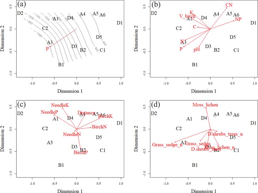
L. Matkala et al.: Soil total phosphorus and nitrogen explain vegetation community composition 1537
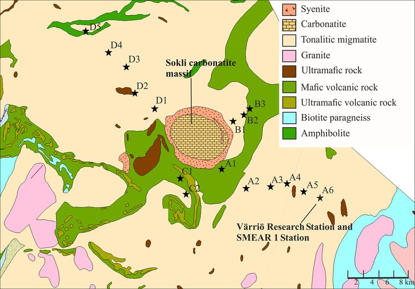
Figure 1. Geological map of the research area. Plots are marked with black stars. The easternmost plot is located at the SMEAR 1 Station.
(source: Hakku Service, https://hakku.gtk.fi/en/locations/search, last access: 28 February 2019.)
rection is south-west (Ruuskanen et al., 2003). The growing 2.2.1 Sampling of soil
season, when daily average temperature exceeds 5 ◦ C, lasts
from June to September. Soils are haplic Podzols with sandy Altogether, 256 soil samples were collected from 16 plots us-
tills (FAO, 1988). ing a soil corer (inner diameter 5 cm) in June 2015. The soil
was sampled within a 1 m distance from the subplots (see
2.2 Plot set-up and vegetation characterization Liski, 1995). The soil cores were separated by visual criteria
into four soil horizons: the top layer, which is a mixture of lit-
The distance between two plots depended on the topogra- ter and decomposing organic layer (F); the humus layer (O);
phy and existing roads, but generally it was about 2 km. A the eluvial layer (A); and the illuvial layer (B) (see Köster
plot consisted of four clusters, each including three 1 m2 et al., 2014). The rocky soil and shallow humus layer made
subplots for observations and sampling (Fig. 2). The size it impossible to sample the mineral soil layers in some clus-
of the whole plot was 30 m × 30 m. We recorded all tree ters. The soil samples from each horizon were combined into
species growing on the plots, measured their heights and composite samples in each cluster in the field. The composite
diameter at breast height (dbh) (equivalent to a height of samples were air-dried, except for the organic F and O hori-
1.3 m) (Table 1). Stem volumes were estimated using the zons, which were dried at 60 ◦ C for 48 h. Dried mineral soils
equations of Laasasenaho (1982). We estimated tree age by were sieved with a 2 mm sieve, and the F and O horizons
measuring dbh and examining the existing approximated tree were milled before storing in a dry place for further analy-
age from plot A6 at SMEAR 1, where the mature trees are ses.
about 70 years old. We considered trees with dbh 1–9.9 cm
as young, 10–14.9 cm as middle-aged and > 15 cm as old. 2.2.2 Sampling of needles and leaves
We visually assessed the cover (percent surface area) and
counted the number of plant species in the understorey veg- Five pines and five spruces per plot were chosen for nee-
etation per plot in all 12 subplots in the summers of 2014 dle sampling in September 2015, when the needle growth
and 2015 (Appendix B). We used a 1 m2 frame to delineate had ended. If less than five trees per species were present,
the subplot (Salemaa et al., 1999). All species in the bottom all of them were chosen. Three branches (length approxi-
layer (bryophytes and lichens) and field layer (dwarf shrubs, mately 50 cm) were taken from the upper third of the canopy
tree seedlings, grasses, sedges and forbs of height < 50 cm) using a branch saw. We took only second-order branches
were included. because cutting of first-order branches would have been
too destructive to the trees (see Helmisaari, 1990). Nee-
www.biogeosciences.net/17/1535/2020/ Biogeosciences, 17, 1535–1556, 2020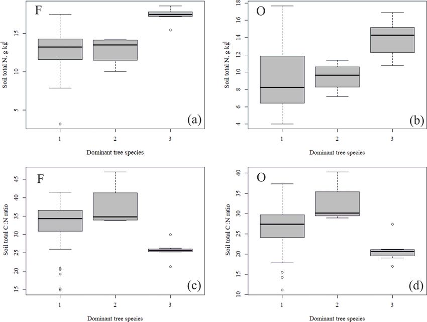
1538                          L. Matkala et al.: Soil total phosphorus and nitrogen explain vegetation community composition

Table 1. Tree species composition of the research plots (dbh = diameter at breast height).

   Plot   Trees ha−1      Basal area of   Total volume of         Volume of           Volume of          Volume of    Average dbh      Average dbh    Average dbh
                       trees (m2 ha−1 )   trees (m3 ha−1 )   pine (m3 ha−1 )   spruce (m3 ha−1 )   birch (m3 ha−1 )   of pine (cm)   of spruce (cm)   of birch (cm)
   A1          1300                 10                 75               44                  0.02              30.7             10              1.8               7
   A2          1200                 12                 78              69.2                  2.3               6.9            9.1              6.5             5.7
   A3           900                  8                 46                 –                  0.5              45.5              –              6.4             9.1
   A4           600                 16                130              83.7                 35.5              11.2           21.5             11.3               9
   A5          1200                 17                125              94.5                 20.9              10.0           18.7              8.4             6.2
   A6           500                 10                 54              53.7                    –               0.7           16.7                –             3.9
   B1           300                  1                  3               2.8                 0.07                 –           13.4              5.6               –
   B2           300                  5                 33              32.6                    –                 –           18.2                –               –
   B3           500                 17                128             127.9                  0.2               0.4           19.2              6.8             5.7
   C1           800                  3                 14              14.3                    –                 –            6.1                –               –
   C2          1100                 14                105              47.1                 41.1              17.7           21.6             12.1               7
   D1           700                 14                 99              99.3                    –              0.03           11.9                –             3.3
   D2          1100                  9                 48                 –                    –                48              –                –             9.8
   D3           500                  4                 18              15.3                    –               2.5            8.5                –             9.2
   D4           300                  7                 43              13.6                 17.2              12.3           21.5              22              9.9
   D5           700                 11                 98              98.3                    –                 –           11.4                –               –

                                                                                          We sampled green birch leaves in July 2015 and sampled
                                                                                      leaf litter in September 2015. Approximately 10 green leaves
                                                                                      from 10 different trees were picked and combined (Rautio
                                                                                      et al., 2010). Only mature, undamaged leaves were chosen.
                                                                                      Birch litter was collected under the same tree canopies from
                                                                                      which the green leaves had been taken and in approximately
                                                                                      the same number as the green leaf samples. We aimed to take
                                                                                      litter leaves shed in the current year, so that they were de-
                                                                                      composed as little as possible. Green and litter leaves were
                                                                                      dried at 65 ◦ C for 48 h and manually cleaned of extra mate-
                                                                                      rial, such as soil particles and needles. The needles and the
                                                                                      few soil particles attached on the litter leaves were removed
                                                                                      with tweezers. The green leaves did not need cleaning. The
                                                                                      litter leaves were also rather clean, as it had rained at the
                                                                                      time of sampling. After cleaning, the leaves were milled and
                                                                                      stored in a dry place for further analyses. Needles and leaves
                                                                                      were sampled at a different time than the soil. Both needle
                                                                                      (e.g. Helmisaari, 1990) and soil nutrient contents vary be-
                                                                                      tween the seasons. However, as all soil and all needle sam-
                                                                                      pling was conducted at the same time of the season, the com-
                                                                                      parison between the plots was not hindered.

                                                                                      2.3     Laboratory analyses

                                                                                      Total element contents of potassium (K) and P were analysed
                                                                                      from soil and foliar samples by inductively coupled plasma
Figure 2. Set-up of each research plot with clusters and subplots                     optical emission spectrometry. For this analysis, the samples
within clusters. Trees were measured from the whole 30 m × 30 m                       were first wet combusted. A 1 g amount of mineral soil sam-
area.                                                                                 ple and 0.3 g of organic sample were combusted with 1 mL
                                                                                      of H2 O2 and 10 mL HNO3 and heated in a microwave oven.
                                                                                      The samples were then filtered with Whatman Grade 589/3
dle age classes (C = current year; C + 1 = 1-year-old nee-                            filter paper and stored in plastic bottles in a cooler until they
dles; C + 2 = 2-year-old needles) were separated from each                            were analysed.
branch and dried at 65 ◦ C for 48 h, milled and stored in a                               Total carbon (C) and N were analysed directly from dried
dry place for further analyses. The samples were combined                             and milled foliar samples and from the F and O soil layers.
so that there was one C, one C + 1 and one C + 2 composite                            Samples of 2–3 mg were measured and analysed with an el-
needle sample per tree.                                                               ement analyser, which uses a high-temperature combustion

Biogeosciences, 17, 1535–1556, 2020                                                                              www.biogeosciences.net/17/1535/2020/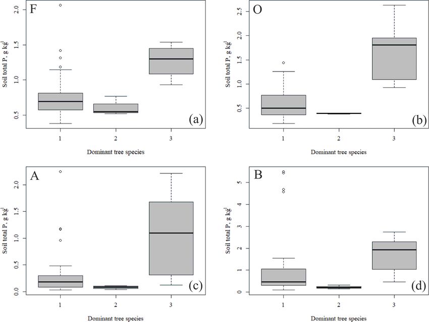
L. Matkala et al.: Soil total phosphorus and nitrogen explain vegetation community composition                                             1539

Figure 3. Soil total phosphorus (P) contents of the research plots (based on dominant tree species) in different soil horizons. Species 1 = pine,
2 = spruce and 3 = birch.

method with subsequent gas analysis of CN (VarioMax, El-                   fects and plot as random effect. Soil total P needed to be log-
ementar Analysensysteme GmbH, Germany). Soil pH was                        transformed, while for N and C : N the visual inspection of
measured from two O layer samples per plot, and their av-                  residual plots (Fig. C1 in Appendix) did not reveal obvious
erage value was used. A total of 20 mg of dried sample was                 deviations from homoscedasticity or normality. We obtained
mixed together with ultrapure water (50 mL). The suspension                p values for the fixed effects by likelihood ratio tests, where
was covered and left standing for 24 h, and pH was measured                the full model with all the fixed effects was tested against
with a glass electrode.                                                    a model where each fixed effect was removed in turn. We
                                                                           used package lme4 (Bates et al., 2015) in R programme 3.4.3
2.4   Statistical analyses                                                 (R Development Core Team, 2017) for building the models.
                                                                           Pseudo R 2 values for the models were calculated by using
We used one-way analysis of variance (ANOVA) and                           package r2glmm (Jaeger, 2017). The models took the follow-
Tukey’s honest significant difference post hoc test for                    ing form:
analysing the plot-wise differences in needle element con-
                                                                           SCP,N,CN = B0 + Bdt + Bta + Bg + Bh + ∈,                          (1)
tents. Plot-averages of needle elemental contents were calcu-
lated across all needle age classes and both conifer species.              where SCP,N,CN is the soil nutrient content (total P or N or
One-way ANOVA was also used in analysing differences be-                   C : N ratio), B0 denotes a fixed intercept parameter, Bdt de-
tween the needle age classes. We grouped the plots based on                notes the fixed unknown parameters associated with the dom-
their dominant tree species into pine, birch and spruce plots              inant tree species, Bta denotes the fixed unknown parameters
and calculated the average soil nutrient contents in each hori-            associated with the age of the dominant tree species, Bg de-
zon in these plots. We then compared the nutrient contents in              notes the fixed unknown parameters associated with the rock
each soil horizon with one-way ANOVA.                                      parent material and Bh denotes the fixed unknown parame-
   We tested the effects of environmental variables on soil                ters associated with the soil horizon. The random effect ∈ is
total P and N contents and C : N with linear mixed-effect                  assumed to take the following form:
models. We used dominant tree species, estimated age class,
rock parent material (Fig. 1), and soil horizon as fixed ef-               ∈= ∝p + u,                                                        (2)

www.biogeosciences.net/17/1535/2020/                                                                 Biogeosciences, 17, 1535–1556, 2020
1540 L. Matkala et al.: Soil total phosphorus and nitrogen explain vegetation community composition
where ∝p denotes the random parameters related to the re- spruce (Table D1). Against our expectations, the needle P
search plot and u is an unobservable error term. Random ef- contents of both conifer species were rather similar across
fect parameters and the random error term are assumed to fol- plots (Table D2). On the other hand, N and C contents, as
low normal distributions ∝p ∼ N (0, σp2 ) and u ∼ N 0, σu2 .
well as the C : N ratio of the conifers, showed some between-
We calculated plot-wise averages from the percentage plot variation (pL. Matkala et al.: Soil total phosphorus and nitrogen explain vegetation community composition 1541
Figure 4. Soil total N content (a, b) and soil C : N ratio (c, d) of the research plots (based on dominant tree species) in soil horizons F and O
(species 1 = pine; species 2 = spruce; and species 3 = birch.
Table 2. Average foliar element contents (g kg−1 ) of the three major nutrients and C, and the relationships of C : N and N : P with standard
deviations. Needle age classes: C = current year; C + 1 = 1-year-old needles; C + 2 = 2-year-old needles.
C N P K C:N N:P
Pine C 510.0 (3.70) 14.10 (0.80) 1.40 (1.40) 4.50 (9.10) 36.0 (1.90) 10.0 (1.10)
Pine C + 1 510.0 (7.30) 13.80 (0.90) 1.20 (0.80) 3.70 (3.70) 38.0 (2.40) 11.80 (1.10)
Pine C + 2 480.0 (140.0) 12.10 (3.70) 1.2 (0.90) 3.50 (3.30) 36.6 (11.20) 10.60 (3.30)
Spruce C 500 (3.80) 12.0 (1.00) 1.70 (0.20) 6.40 (0.90) 42.0 (3.50) 7.10 (0.70)
Spruce C + 1 440.0 (170.0) 10.70 (4.20) 1.50 (0.20) 4.20 (0.90) 37.0 (14.50) 7.30 (2.90)
Spruce C + 2 440.0 (165.0) 10.10 (3.90) 1.40 (0.20) 3.70 (0.80) 39.2 (14.90) 7.50 (3.00)
Birch, green 470.0 (3.40) 25.0 (1.20) 2.60 (0.30) 8.20 (1.50) 19.0 (1.0) 9.80 (1.0)
Birch, litter 490.0 (6.0) 10.10 (1.40) 1.30 (0.50) 2.40 (1.00) 50.0 (7.40) 8.50 (2.10)
had a higher number of forbs and grasses growing on them while the moisture gradient followed the second dimension.
than the plots positioned on the right-hand side of each panel Moisture-demanding species, such as Equisetum sylvaticum,
(Fig. 6a, b). Species such as Calamagrostis epigejos, Carex are located in the upper part of Fig. 6b, and those tolerating
spp., Rubus arcticus and Luzula pilosa had relatively high drier conditions, such as Stereocaulon tomentosum, are lo-
coverage on the left of each panel. Plots further to the right in cated in the lower part of the ordination space in Fig. 6b. An-
each panel had more species that tolerate poor and dry grow- other moisture gradient, expressing specific paludified condi-
ing conditions, such as Cladonia lichens. The tree species tions, seemed to follow the third dimension. Peatland species
also changed from right to left, as the plots on the right were like Sphagnum angustifolium and Aulacomnium palustre are
dominated by pine, whereas furthest on the left in plot D2, located in the upper part of Fig. 6d, and species preferring dry
birch was the only tree species present. In general, the fer- conditions, such as Cetraria islandica, are in the lower part
tility trend in the vegetation followed the first dimension, of Fig. 6d. Considering all three dimensions of ordination
www.biogeosciences.net/17/1535/2020/ Biogeosciences, 17, 1535–1556, 20201542 L. Matkala et al.: Soil total phosphorus and nitrogen explain vegetation community composition
4 Discussion
All the plant species growing in the study plots were com-
mon forest species in Finland (e.g. Reinikainen et al., 2000,
Finnish Biodiversity Information Facility https://laji.fi/en,
last access: 20 March 2019) (Appendix B). However, in some
plots the structure and abundance of species in the under-
storey clearly differed from the surrounding, more typical
northern boreal forests. We found evidence that the number
of species in the group of grasses and sedges, as well as the
cover (percent of the surface) of the same plant group, had
a higher positive correlation with humus P content than N
content (Fig. 5). However, both of these nutrients were im-
portant factors explaining the vegetation composition in the
ordination configuration (Fig. 7), which supports our first hy-
pothesis. We also found that the humus C : N ratio correlated
negatively with the abundance and species composition in
the understorey. Additionally, Salemaa et al. (2008) have ob-
served that total N and the C : N ratio of the humus layer
explained most large-scale vegetation variation across sev-
eral forest sites in Finland. They also measured extractable
soil P, which seemed to have more power to explain vege-
tation patterns in northern Finland than in southern Finland.
Soil P availability was one of the key factors in plant com-
Figure 5. Correlation (Pearson) including soil elements (K, P, C : N, munity variation in alpine habitats in Troms, northern Nor-
pH, C, N : P), number of species (with _n in the end of the name) way (Arnesen et al., 2007), where a higher variety of lichen
and total percentage cover of plant species in different layers (moss species and the frequency of occurrence of Salix herbacea
and lichen, grasses, herbs and sedges, dwarf shrubs and trees), nee-
and certain sedge and grass species were explained by higher
dle elements (N, P, K), plot distance from Sokli, green birch ele-
ments (N, P, K) and birch litter elements (N, P, K). Levels of signif-
availability of P in soil. We conclude that the possible aerial
icance: ∗ = 0.05; ∗∗ = 0.01; ∗∗∗ = 0.001. Positive correlations are deposition of phosphate from the mine in Sokli could lead to
displayed in blue, and negative correlations are displayed in red. changes in plant species composition and abundance if high
Colour intensity and the size of the circle are proportional to the amounts of P are deposited into the ecosystem surrounding
correlation coefficients. the mining region.
Our second hypothesis stated that the N and P contents of
the topmost soil layers correlate with the N and P contents
space, the generalist species, such as Pleurozium schreberi of foliar biomass, but our results (Fig. 5, Table D2) did not
and Vaccinium myrtillus are located in the middle of Fig. 6b, support this hypothesis. The reason could be that we mea-
d. sured total contents of N and P in soil instead of the plant-
The vector arrows fitted to the ordination space (Fig. 7c, available contents of these nutrients. The plant-available con-
d) depict the maximum correlations between environmen- tents of these nutrients might have given different results.
tal variables and plot ordination. The length of an arrow in- Perhaps plant species composition in ground vegetation is
dicates the magnitude and direction of the polarity (plus– sensitive to even small additions of available N and P in the
minus) of the correlation. The highest correlations occurred upper soil layers where the roots occur, whereas higher con-
between the plot-wise average P content of the soil O hori- tents of these elements are required for there to be any ef-
zon and the ordination pattern of the plots (Table C4). The fect on the needles. The P and N levels of our needle sam-
isocline gradient of soil P in relation to the ordination pat- ples were similar to those previously measured in Finland
tern was almost linear (Fig. 7a). Vectors of soil pH, N and P (Helmisaari, 1990; Merilä and Derome, 2008; Moilanen et
content all increased towards the more fertile plots, but the al., 2013). The higher P contents of C needles compared
vectors of soil C : N and N : P went in opposite directions with older needles is common for conifers and occurs be-
(Fig. 7b) indicating poor soil conditions. The average total cause the dry weight in recently matured needles increases
number of grass, forb, and sedge species and their coverage faster than the transportation of P to the needles (Helmisaari,
in the study plots also increased towards the more fertile plots 1990). The N contents of both green birch leaves and leaf lit-
(Fig. 7d). ter agreed with those reported by Ferm and Markkola (1985).
The P contents of the green leaves were higher than mea-
sured in that study (approximately 2.0 g kg−1 ). Although the
Biogeosciences, 17, 1535–1556, 2020 www.biogeosciences.net/17/1535/2020/L. Matkala et al.: Soil total phosphorus and nitrogen explain vegetation community composition 1543 Figure 6. Ordination pattern of the research plots in dimensions 1 and 2 (a, b) and dimensions 1 and 3 (c, d). Panels (a) and (c) give plot ordinations, and (b) and (d) give weighted averages of the most abundant species (highest cover percentage of the surface). Less abundant species are marked with light-coloured crosses. The names of species are combinations of the first four letters of their genera and species names (e.g. Solivirg stands for Solidago virgaurea). The tree species mentioned in the figure are at seedling stage. In (a) plots A4, B3, and A2 and in (c) plots A1 and B1, B2 and B3, and A4 and A2 were located on top of each other. foliar N and P contents were not reflected in the uppermost P (Rinnan et al., 2008) contents in the organic soil layer in soil layers, our results support the third hypothesis, and the those subarctic heaths, where Hylocomium splendens dom- occurrence of birch correlates positively with the N and P inated the moss layer. These results imply that birch is an content of the top layers of soil (Table C2). The plots dom- important factor in recycling and providing P to the soil in inated by birch had significantly higher total P content in certain types of northern forest sites. all but the B layer compared with plots dominated by the In general, the spatial variation in soil element contents conifers (Figs. 3 and 4). Birch leaves were a major source between plots was high, emphasizing the heterogeneity of of litter in the plots where soil P was high. These findings soil fertility level (Figs. C2 and C3). As our results showed, are supported by the study of Lukina et al. (2019), which this heterogeneity can partially be explained by the dominant found that the extractable P content of organic soil layers tree species of the research plot, which especially affects the was significantly higher in birch- and spruce-dominated for- topmost soil layers. According to the nutrient-uplifting hy- est sites than in sites dominated by pine in north-western pothesis (Jobbágy and Jackson, 2004), trees and other veg- Russia. Viro (1955) found that the leaf litter of birch had re- etation can transport minerals such as P and K from the markably high P content compared with other Finnish tree deep soil layers to the surface of soils. The P contents of species. The litter P contents in this study were near the ap- soil samples (Table C1) in our study (1.80–2.60 g kg−1 in proximately 1.50 g kg−1 that Ferm and Markkola (1985) mea- the O horizon) fell mostly in the category we could expect sured from a 40-year-old forest but much less than those re- based on the literature. The P content of the humus layer in ported from younger forests. In a litter experiment in Abisko southern Finnish forest soil has been observed to vary be- (northern Sweden), the addition of birch litter increased both tween 0.80 and 2.10 g kg−1 (Mäkipää, 1999), whereas differ- the total P (Sorensen and Michelsen, 2011) and the available ent studies in northern Finland have found the P contents of www.biogeosciences.net/17/1535/2020/ Biogeosciences, 17, 1535–1556, 2020
1544                       L. Matkala et al.: Soil total phosphorus and nitrogen explain vegetation community composition

Figure 7. Ordination pattern with smooth surface fit and linear vector fit of soil phosphorus (P) in the O layer (a), linear vector fits of soil
element contents in the O layer (b), linear vector fits of foliar data and plot distance from Sokli phosphate ore (c), and linear vector fits of
number of species in different layers of understorey (d). Moss_lichen includes moss and lichen species; Grass_sedge includes forb, grass,
and sedge species; and D.shrubs_trees includes dwarf shrubs and tree seedlings. Plots A4, B3 and A2 were located on top of each other, and
only A4 is shown.

0.39–3.00 g kg−1 in the organic topsoil (Mikkola and Sep-                 ratio of 40 from a northern Finnish forest site, which is higher
ponen, 1986; Reimann et al., 1997). Most of our plots had                 than we measured.
the highest P content in the organic soil layers, implying that              Our study area does not represent typical northern boreal
decaying plant parts were a major source of P added to the                forest, as it was located near the phosphate massif, the effect
soil. Low Arctic soils tend to have organic P as the primary              of which needs to be considered. Talvitie (1979), who used
form of P (Weintraub, 2011). The content of organic P usu-                remote sensing for a geobotanical survey of the Sokli mas-
ally gets smaller in the deeper soil (Achat et al., 2009). Thus,          sif, found that the density of occurrence of birch, juniper and
if P content is high in deep soil layers, as it was in some               grass species increased when carbonatite was the underlying
of our plots, the source of P in these plots is most likely               rock material. The surveys related to Natura 2000 (Standard
to be the underlying bedrock. The plot-wise average pH of                 Data Form FI1301512 and FI1301513) stated that the Tör-
our soil samples agreed with that measured by Köster et                   mäoja and Yli-Nuortti areas, where plots B1–B3 and A1–A2
al. (2014), who conducted their study at the same site, albeit            were, have a high occurrence of grass species and a sparse
not in the same plots. The pH of the soil humus layer cor-                birch-dominated tree cover due to carbonatite in the soil.
related positively with the number of grass, herb and sedge               According to the geological map (Fig. 1), only small parts
species, which is reasonable, since higher pH usually implies             in the western ends of both the Törmäoja and Yli-Nuortti
a more fertile site. The soil N contents from our plots agreed            Natura areas are located on top of carbonatite rock. Simi-
with the reported values from Finnish forest sites (Merilä and            larly, the map shows that those of our plots where the vege-
Derome, 2008; Salemaa et al., 2008), ranging between 9.8                  tation community was reminiscent of Sokli have something
and 12.8 g kg−1 . Salemaa et al. (2008) reported a soil C : N             other than carbonatite as the rock parent material. However,
                                                                          all of our plots have metamorphic (tonalitic migmatite and

Biogeosciences, 17, 1535–1556, 2020                                                              www.biogeosciences.net/17/1535/2020/
L. Matkala et al.: Soil total phosphorus and nitrogen explain vegetation community composition 1545 amphibolite) or igneous (mafic volcanic and ultramafic) rock 5 Conclusions as the parent material, and phosphate mineral apatite can oc- cur in such rocks (Walker and Syers, 1976). It is likely that We found that the total P content of the soil humus layer was these types of rock materials leach more phosphate than other an important factor explaining the community composition types of bedrock (Arnesen et al., 2007). Thus, the rocks out- of forest understorey vegetation near the Sokli phosphate ore side of the carbonatite massif may also have locally high P in Finnish Lapland. The plots with high soil total P in the hu- content, which affects the P content of the soil. The mixed- mus layer had birch as the dominating tree species. As green effect model factor “geology” did not consider this, which birch leaves and leaf litter also had high contents of P, we could be the reason why it was not important in explaining suggest that the litter caused the high total P contents in the soil P content. humus layer. As climate change and the possible mining ac- The baseline status and the current vegetation composition tivities may affect the nutrient and vegetation dynamics in the of our research site was worth studying for several reasons. studied region, the research that we carried out has an impor- We conducted our study in a region which has for decades tant role in both clarifying the current situation and forming been under more or less heated discussion related to whether a baseline for evaluating the magnitude of changes in the fu- mining activities will begin or not. The site is very remote ture. and the plan is to move the material from the mine to loca- tions of further production by trucks (Pöyry Environment, 2009). In addition to the aerial deposition from the mine, this could increase the dust and pollution caused by trans- portation, the amount of which is currently minimal. The ef- fects of mining on the surrounding ecosystem and its vegeta- tion composition can be unpredictable when combined with the changes caused by climate change. High-latitude regions are considered more vulnerable to climate change than more southern regions (Hartmann et al., 2013). Soil microbial ac- tivity may change due to a warmer climate, and therefore N may become more available from organic sources (Rustad et al., 2001). This, together with high soil P, may induce growth and affect vegetation dynamics. Climate change has already caused variation in the vegetation at high latitudes, as decidu- ous shrub coverage has expanded in the Arctic region (Sturm et al., 2001; Park et al., 2016). Greater deciduous shrub cover causes increased leaf litter input, which in turn may bring more nutrients that are recyclable to the ecosystem. www.biogeosciences.net/17/1535/2020/ Biogeosciences, 17, 1535–1556, 2020
1546                     L. Matkala et al.: Soil total phosphorus and nitrogen explain vegetation community composition

Appendix A

Table A1. Meteorological parameters from Värriö. Values for the
climatological normal period are from Pirinen et al. (2012). Grow-
ing degree day sum was calculated as the average daily tempera-
ture (average of daily maximum and minimum temperatures) above
the 5 ◦ C base temperature, accumulated on a daily basis over the
year. Negative values are treated as 0 and ignored. SWE stands for
snow water equivalent. a Data from SMEAR 1 Station. b Data from
SMEAR 1 Station (only 2009–2015). All other data are collected
from the Värriö Subarctic Research Station by the Finnish Meteo-
rological Institute.

                                      2014     2015    Climatological
                                                       normal period
                                                        (1981–2010)
 Average annual temperature (◦ C)     0.84     0.95              −0.5
 Average min. temperature (◦ C)      −2.09     −1.7              −3.5
 Average max. temperature (◦ C)        3.9       3.8              2.6
 Growing degree day sum                860      640               680
 Total precipitation (mm)              610      660               601
    Snowfall (mm, SWE)a                390      420              400b
    Rainfall (mm)                      220      240              190b

Biogeosciences, 17, 1535–1556, 2020                                              www.biogeosciences.net/17/1535/2020/
L. Matkala et al.: Soil total phosphorus and nitrogen explain vegetation community composition 1547 Appendix B Table B1. Average coverage (percentage of surface area) of under- storey plant species per plot. Species A1 A1 A3 A4 A5 A6 B1 B2 B3 C1 C2 D1 D2 D3 D4 D5 Pleurozium schreberi 43.3 51.3 39.6 59.3 44.4 57.1 25.0 24.7 64.7 9.0 38.8 0.3 1.2 53.5 14.5 38.7 Hylocomium splendens 38.7 8.3 22.8 9.6 3.3 1.7 – 3.8 1.3 – 28.9 – 44.6 – 14.5 – Dicranum scoparium – 12.6 – 4.2 5.9 10.7 1.6 2.8 – 8.3 – 72.9 – 1.0 9.7 4.1 Dicranum polysetum – – – – 0.2 0.1 – 0.9 0.8 – – – – – 0.6 0.4 Dicranum majus – – – 1.1 – – – – – – – – – – – 1.3 Barbilophozia barbata – – – 0.1 0.7 0.6 – – – – – – – 0.2 0.2 5.8 Polytrichum strictum – – 2.8 – – – 5.0 5.3 – 0.8 – – – 2.1 – – Polytrichum commune 3.4 0.4 0.7 0.1 – – 0.4 – – – 1.4 – 23.4 4.0 4.9 0.1 Aulacomnium palustre – – – – – – – – – – – – – 3.7 – – Sphagnum angustifolium – – – – – – – – – – 1.0 – – – – – Sphagnum girgensohnii – – – – – – – – – – 0.3 – – – – – Sphagnum capillifolium – – – – – – – – – – – – – 0.2 – – Ptilidium ciliare – – – – – 1.1 – – – – – – – – – – Peltigera aphthosa 1.1 – – – 1.0 – 0.6 0.7 0.4 – – – – – 0.1 – Peltigera rufescens – – 0.2 – – – – – – – – – – – – – Peltigera neopolydactyla – – – – – – 10.9 0.1 – – – – – – – – Nephroma arcticum – 2.3 1.0 3.9 – – 6.1 1.5 0.5 – – – – 0.5 0.1 1.3 Umbilicaria deusta – – – – – – – 0.1 – – – – – – – – Cladonia rangiferina 0.3 1.0 0.3 1.6 1.5 2.0 6.2 2.8 1.6 31.0 – 3.8 – 5.2 0.3 5.3 Cladonia cornuta – – 0.1 – 0.2 – 0.1 0.2 – 0.1 – 0.2 – – – 0.3 Cladonia stellaris – – – – – – – – – – – – – – – – Cladonia deformis – – – – – – – 0.1 – 0.6 – – – – – 0.1 Cladonia crispata var. crispata – – – – – – – – – – – – – – – – Cetraria islandica – 0.1 – – – – – – – – – – – – – – Stereocaulon tomentosum – – – – – – 4.7 2.2 – – – – – – – – Linnaea borealis – – – – 0.3 0.2 – – 0.1 – – – – – – – Vaccinium myrtillus 1.2 4.3 – 10.7 14.7 27.7 – 5.2 2.3 1.4 8.4 1.3 2.7 18.8 6.0 6.9 Vaccinium vitis-idaea 15.3 26.8 5.6 22.2 11.9 5.2 1.3 5.5 21.6 5.7 3.4 28.2 25.8 4.0 7.4 4.4 Vaccinium uliginosum 7.1 0.8 – – – 0.5 15.5 5.3 2.3 2.9 34.3 – 11.6 41.7 6.3 1.5 Empetrum nigrum 2.7 9.8 0.8 8.4 14.1 12.4 – 9.6 32.8 9.3 14.5 15.0 4.1 40.4 7.0 6.9 Arctostaphylos uva-ursi – – – – – – 10.7 0.2 0.4 – – – – – – – Arctostaphylos alpina – – – – – – – – – – – – – – – – Betula nana 23.9 6.3 1.3 – – – – – – – 2.2 – – 2.7 – – Calluna vulgaris – – – – – 0.5 – – – 0.2 – – – 0.6 – 0.4 Rhododendron tomentosum – – – – – – – – – – – – – 0.8 3.6 – Juniperus communis 0.9 – 0.8 0.6 – – 5.7 0.3 2.2 – 2.5 – 3.7 – – – Picea abies – – – 0.5 – – – – – – – – – – – – Pinus sylvestris – – – – – – 1.6 0.8 – 2.1 0.1 0.9 – 0.8 – 0.7 Betula pubescens 1.1 0.2 1.4 – – 0.4 2.5 0.7 – – – – – 0.2 0.1 – Populus tremula – – – – – 0.4 – – – – – – – – – – Diphasiastrum complanatum – – – – – 0.1 0.7 – – – – – – – – – Trientalis europaea – 0.1 0.7 – – – – – – – – – 3.4 – – – Melampyrum sylvaticum – – 0.3 – – – 0.1 – – – – – – 0.1 – – Solidago virgaurea – – 1.1 – – – 1.2 – – – 0.2 – 0.7 – – – Rubus arcticus – – 0.6 – – – – – – – – – 3.2 – – – Rubus chamaemorus – – – – – – – – – – 0.4 – – – – – Antennaria dioica – – – – – – 1.2 – – – – – – – – – Orthilia secunda – – – – – – – – – – 0.1 – – – – – Chamaenerion angustifolium – – – – – – – – – – – – 0.7 – – – Galium uliginosum – – – – – – – – – – – – 0.1 – – – Geranium sylvaticum – – – – – – – – – – – – 0.2 – – – Chelidonium majus – – – – – – – – – – – – 0.1 – – – Comarum palustre – – – – – – – – – – – – 0.3 – – – Equisetum sylvaticum 0.1 – – – – – – – – – – – 0.8 – 0.2 – Luzula pilosa 0.6 – 0.4 – – – 1.8 – – – 0.2 – 2.4 0.3 – – Elymus repens – – – – – – – – – – – – – – – – Deschampsia flexuosa 3.5 0.6 10.3 0.6 – 0.2 2.1 0.3 0.4 – 2.8 – 15.9 7.1 2.2 0.2 Festuca rubra – – – – – – – – – – – – 1.9 – – – Calamagrostis epigejos – – – – – – – – – – – – 5.4 – – – Carex digitata – – – – – – – – – – – – 0.6 – – – Carex nigra – – – – – – – 0.2 – – – – – – – – Carex canescens – – – – – – – – – – 0.5 – 3.4 – – – Carex globularis – – – – – – – – – – – – – 1.7 – – www.biogeosciences.net/17/1535/2020/ Biogeosciences, 17, 1535–1556, 2020
1548                      L. Matkala et al.: Soil total phosphorus and nitrogen explain vegetation community composition

Appendix C: Soil element contents within and across
plots and statistical analyses

Figure C1. The fitted values vs. residuals: q–q plots and histograms
of residuals from the mixed-effect models (the upper row shows val-
ues for phosphorus, and the lower row shows values for nitrogen).

Biogeosciences, 17, 1535–1556, 2020                                               www.biogeosciences.net/17/1535/2020/
L. Matkala et al.: Soil total phosphorus and nitrogen explain vegetation community composition                1549

Figure C2. Soil total P content within plots in different soil layers.

www.biogeosciences.net/17/1535/2020/                                            Biogeosciences, 17, 1535–1556, 2020
1550                      L. Matkala et al.: Soil total phosphorus and nitrogen explain vegetation community composition

Figure C3. Soil total N content and C : N ratio within plots in the F
and O layers.

Biogeosciences, 17, 1535–1556, 2020                                               www.biogeosciences.net/17/1535/2020/
L. Matkala et al.: Soil total phosphorus and nitrogen explain vegetation community composition                                           1551

Table C1. Average total contents of elements (g kg−1 ) in soil layers
and their standard deviations in parentheses. All plots are included.

                        K            P            N             C         C:N             N:P        pH
 F layer    0.83 (0.30)     0.81 (0.32)   13.3 (2.9)    420 (98)        32 (6.8)   17.8 (5.5)           –
 O layer    0.49 (0.22)     0.72 (0.50)    9.9 (3.7)   260 (106)        26 (5.7)   17.2 (7.3)   3.7 (0.2)
 A layer    0.32 (0.22)     0.38 (0.51)            –           –               –            –           –
 B layer    0.59 (0.23)     0.10 (0.13)            –           –               –            –           –

Table C2. Statistical differences of soil elements in each soil layer
of different plots, grouped by their dominant tree species. Levels of
significance: ∗ = 0.05; ∗∗ = 0.01; ∗∗∗ = 0.001.

            P                                          N                                           C:N
 F layer    birch and pine∗∗∗ birch and spruce∗∗       birch and pine∗∗∗ birch and spruce∗∗        birch and pine∗∗ birch and spruce∗∗
 O layer    birch and pine∗∗∗ birch and spruce∗∗∗      birch and pine∗∗                            birch and pine∗ birch and spruce∗∗
 A layer    birch and pine∗∗∗ birch and spruce∗        –                                           –
 B layer    –                                          –                                           –

Table C3. Results from the mixed-effect models, testing the effects
of environmental variables on soil total P and N content and C : N
ratio. The tested variables were dominant tree species of the re-
search plot, estimated tree age, rock parent material (geology) and
soil layer. Random effect was related to plot number. Pseudo-R 2
was calculated based on Nakagawa and Schielzeth (2013), John-
son (2014), and Jaeger et al. (2016).

 Soil total P content
 Fixed effects                      Chi square value           p value      Pseudo-R 2
 Factor (dominant tree species)               7.9009         0.01925               0.45
 Factor (tree age)                            4.0408          0.1326
 Factor (geology)                             4.8171         0.08995
 Factor (soil layer)                          155.97    2.20 × 10⁻¹⁶
 Soil total N content
 Fixed effects                      Chi square value           p value      Pseudo-R 2
 Factor (dominant tree species)               4.9146         0.08567                0.2
 Factor (tree age)                            2.1769          0.3367
 Factor (geology)                             2.2291          0.3281
 Factor (soil layer)                          53.408    2.71 × 10⁻¹³
 Soil total C : N ratio
 Fixed effects                      Chi square value           p value      Pseudo-R 2
 Factor (dominant tree species)               4.2076            0.122               0.2
 Factor (tree age)                            1.3484          0.5096
 Factor (geology)                             0.3339          0.8462
 Factor (soil layer)                          60.036    9.31 × 10⁻¹⁵

www.biogeosciences.net/17/1535/2020/                                                                 Biogeosciences, 17, 1535–1556, 2020
1552 L. Matkala et al.: Soil total phosphorus and nitrogen explain vegetation community composition Table C4. Linear correlations of element contents of soil, needles, and leaves; number of species in different vegetation layers; and plot distance from Sokli with the non-metric multidimensional scaling ordination pattern. The group of “grasses and sedges” includes forb, grass, and sedge species and “d. shrubs and trees” includes dwarf shrubs and tree seedlings. Levels of significance: ∗ = 0.1; ∗∗ = 0.05; ∗∗∗ = 0.01. The first seven rows are soil values. Variable R2 p< K 0.225 0.220 P 0.717 0.002∗∗∗ N 0.368 0.087∗ C 0.137 0.461 C:N 0.576 0.012∗∗ N:P 0.431 0.045∗∗ pH 0.386 0.075∗ Needle P 0.440 0.033∗∗ Needle N 0.010 0.927 Needle K 0.465 0.029∗∗ Birch P 0.247 0.213 Birch N 0.104 0.569 Birch K 0.346 0.099∗ Moss and lichen, species number 0.249 0.223 Grasses and sedges, species number 0.738 0.003∗∗∗ D. shrubs and trees, species number 0.181 0.341 Moss and lichen, percentage cover of surface 0.180 0.325 Grasses and sedges, percentage cover of surface 0.248 0.196 D.shrubs and trees, percentage cover of surface 0.250 0.198 Plot distance from Sokli 0.183 0.344 Biogeosciences, 17, 1535–1556, 2020 www.biogeosciences.net/17/1535/2020/
L. Matkala et al.: Soil total phosphorus and nitrogen explain vegetation community composition                           1553

Appendix D: Needle and leaf nutrient contents per plot

Table D1. Statistically significant differences between needle age
group by species (C = youngest needles; C + 1 = 1-year-old nee-
dles; C + 2 = 2-year-old needles) and p
1554                      L. Matkala et al.: Soil total phosphorus and nitrogen explain vegetation community composition

Data availability. We have made all data used in the anal-              Brække, F. H. and Salih, N.: Reliability of Foliar Analyses of Nor-
yses publicly available. All data can be downloaded from                   way Spruce Stands in a Nordic Gradient, Silva Fenn., 36, 489–
https://doi.org/10.23728/b2share (Matkala et al., 2020).                   504, https://doi.org/10.14214/sf.540, 2002.
                                                                        Cajander, A. K.: Über Waldtypen, Acta For. Fenn., 1, 1–175, 1909.
                                                                        Cajander, A. K.: Forest types and their significance, Acta For. Fenn.,
Author contributions. LM and JB planned the study set-up; LM               56, 1–71, 1949.
conducted all fieldwork, laboratory and statistical analyses and led    Dirnböck, T., Grandin, U., Bernhardt-Römermann, M., Beud-
the writing process; MS had a substantial role in guiding the ordi-        ert, B., Canullo, R., Forsius, M., Grabner, M.-T., Holm-
nation analyses and the writing process; and all authors contributed       berg, M., Kleemola, S., Lundin, L., Mirtl, M., Neumann,
to the writing.                                                            M., Pompei, E., Salemaa, M., Starlinger, F., Staszewski, T.,
                                                                           and Uzieblo, A. K.: Forest floor vegetation response to nitro-
                                                                           gen deposition in Europe, Glob. Change Biol., 20, 429–440,
Competing interests. The authors declare that they have no conflict        https://doi.org/10.1111/gcb.12440, 2014.
of interest.                                                            Dupré, C., Wessberg, C., and Diekmann, M.: Species richness in de-
                                                                           ciduous forests: Effects of species pools and environmental vari-
                                                                           ables, J. Veg. Sci., 13, 505–516, https://doi.org/10.1111/j.1654-
                                                                           1103.2002.tb02077.x, 2002.
Acknowledgements. We thank the staff at the Värriö Subarctic Re-
                                                                        FAO: FAO/Unesco Soil map of the world, revised legend, World
search Station for providing full board during the fieldwork, Marjut
                                                                           Soil Resources Report 60, FAO, Rome, 140 pp., 1988.
Wallner for guidance in the laboratory, Jarkko Isotalo for comment-
                                                                        Ferm, A. and Markkola, A.: Hieskoivun lehtien, oksien ja silmu-
ing on the statistical analyses, Jukka Pumpanen and Kajar Köster
                                                                           jen ravinnepitoisuuksien kasvukautinen vaihtelu. Abstract: Nu-
for advice and equipment for the soil sampling, and Olli Peltola for
                                                                           tritional variation of leaves, twigs and buds in Betula pubescens
helping with field-work. We also thank the two anonymous review-
                                                                           stands during the growing season, Folia For., 613, 1–28, 1985.
ers for their helpful comments.
                                                                        Finnish Biodiversity Information Facility: available at: https://laji.
                                                                           fi/en, last access: 20 March 2019.
                                                                        Hakku service: available at: https://hakku.gtk.fi/en/locations/search,
Financial support. The research has been supported by the Maj              last access: 28 February 2019.
and Tor Nessling Foundation and Finnish Centre of Excellence            Hari, P., Kulmala, M., Pohja, T., Lahti, T., Siivola, E., Palva,
(grant nos. 272041, 307331).                                               L., Aalto, P., Hämeri, K., Vesala, T., Luoma, S., and Pulli-
                                                                           ainen, E.: Air pollution in Eastern Lapland: Challenge for an
Open-access funding provided by Helsinki University Library.               environmental measurement station, Silva Fenn., 28, 29–39,
                                                                           https://doi.org/10.14214/sf.a9160, 1994.
                                                                        Hartmann, D. L., Klein Tank, A. M. G., Rusticucci, M., Alexan-
Review statement. This paper was edited by Yakov Kuzyakov and              der, L. V., Brönnimann, S., Charabi, Y., Dentener, F. J., Dlugo-
reviewed by two anonymous referees.                                        kencky, E. J., Easterling, D. R., Kaplan, A., Soden, B. J., Thorne,
                                                                           P. W., Wild, M., and Zhai, P. M.: Observations: Atmosphere and
                                                                           Surface, in: Climate Change 2013: The Physical Science Basis,
                                                                           Contribution of Working Group I to the Fifth Assessment Report
                                                                           of the Intergovernmental Panel on Climate Change, editeb by:
                                                                           Stocker, T. F., Qin, D., Plattner, G.-K., Tignor, M., Allen, S. K.,
References                                                                 Boschung, J., Nauels, A., Xia, Y., Bex, V., and Midgley, P. M.,
                                                                           Cambridge University Press, Cambridge, United Kingdom and
Achat, D. L., Bakker, M. R., Augusto, L., Saur, E., Dousseron,             New York, NY, USA, 159–254, 2013.
  L., and Morel, C.: Evaluation of the phosphorus status of P-          Hedwall, P-O., Bergh, J., and Brunet, J.: Phosphorus and nitro-
  deficient podzols in temperate pine stands: combining isotopic           gen co-limitation of forest ground vegetation under elevated
  dilution and extraction methods, Biogeochemistry, 92, 183–200,           anthropogenic nitrogen deposition, Oecologia, 185, 317–326,
  https://doi.org/10.1007/s10533-008-9283-7, 2009.                         https://doi.org/10.1007/s00442-017-3945-x, 2017.
Arnesen, G., Beck, P. S. A., and Engelskjøn, T.: Soil Acid-             Helmisaari, H.-S.: Temporal Variation in Nutrient Concentrations
  ity, Content of Carbonates, and Available Phosphorus                     of Pinus sylvestris Needles, Scand. J. Forest Res., 5, 177–193,
  Are the Soil Factors Best Correlated with Alpine Vegeta-                 https://doi.org/10.1080/02827589009382604, 1990.
  tion: Evidence from Troms, North Norway, Arct. Antarct.               Hobbie, S. E., Nadelhoffer, K. J., and Högberg, P.: A syn-
  Alp. Res., 39, 189–199, https://doi.org/10.1657/1523-                    thesis: The role of nutrients as constraints on carbon bal-
  0430(2007)39[189:SACOCA]2.0.CO;2, 2007.                                  ances in boreal and arctic regions, Plant Soil, 242, 163–170,
Augusto, L., Achat, D. L., Jonard, M., Vidal, D., and Ringeval, B.:        https://doi.org/10.1023/A:1019670731128, 2002.
  Soil parent material – A major driver of plant nutrient limitations   Hofmeister, J., Hošek, J., Modrý, M., and Roleček, J.: The influence
  in terrestrial ecosystems, Glob. Change Biol., 23, 3808–3824,            of light and nutrient availability on herb layer species richness in
  https://doi.org/10.1111/gcb.13691, 2017.                                 oak-dominated forests in central Bohemia, Plant Ecol., 205, 57–
Bates, D., Maechler, M., Bolker, B., and Walker, S: Fitting Lin-           75, https://doi.org/10.1007/s11258-009-9598-z, 2009.
  ear Mixed-Effects Models Using lme4, J. Stat. Soft., 67, 1–48,
  https://doi.org/10.18637/jss.v067.i01, 2015.

Biogeosciences, 17, 1535–1556, 2020                                                            www.biogeosciences.net/17/1535/2020/
You can also read