Modeling Fine-Scale Cetaceans' Distributions in Oceanic Islands: Madeira Archipelago as a Case Study
←
→
Page content transcription
If your browser does not render page correctly, please read the page content below
ORIGINAL RESEARCH
                                                                                                                                               published: 08 July 2021
                                                                                                                                     doi: 10.3389/fmars.2021.688248

                                            Modeling Fine-Scale Cetaceans’
                                            Distributions in Oceanic Islands:
                                            Madeira Archipelago as a Case Study
                                            Marc Fernandez 1,2* , Filipe Alves 1,3 , Rita Ferreira 1,3 , Jan-Christopher Fischer 4,5 ,
                                            Paula Thake 5 , Nuno Nunes 6 , Rui Caldeira 3 and Ana Dinis 1,3
                                            1
                                             MARE - Marine and Environmental Sciences Centre, Agência Regional para o Desenvolvimento da Investigação Tecnologia
                                            e Inovação (ARDITI), Funchal, Portugal, 2 cE3c/Azorean Biodiversity Group, Departamento de Biologia, Faculdade
                                            de Ciências e Tecnologia, Universidade dos Açores, Ponta Delgada, Portugal, 3 Oceanic Observatory of Madeira (OOM),
                                            Funchal, Portugal, 4 School of Earth Sciences, University of Bristol, Bristol, United Kingdom, 5 Lobosonda - Madeira Whale
                                            Watching, Estreito da Calheta, Portugal, 6 ITI/LARSyS, Técnico Lisboa, Universidade de Lisboa, Lisbon, Portugal

                                            Species distributional estimates are an essential tool to improve and implement
                           Edited by:       effective conservation and management measures. Nevertheless, obtaining accurate
                      Matthew Lewis,        distributional estimates remains a challenge in many cases, especially when looking
   Bangor University, United Kingdom
                                            at the marine environment, mainly due to the species mobility and habitat dynamism.
                       Reviewed by:
        Victoria Paige Van de Vuurst,       Ecosystems surrounding oceanic islands are highly dynamic and constitute a key actor
         Virginia Tech, United States       on pelagic habitats, congregating biodiversity in their vicinity. The main objective of
                      James Waggitt,
   Bangor University, United Kingdom
                                            this study was to obtain accurate fine-scale spatio-temporal distributional estimates
                 *Correspondence:
                                            of cetaceans in oceanic islands, such as the Madeira archipelago, using a long-term
                     Marc Fernandez         opportunistically collected dataset. Ecological Niche Models (ENM) were built using
                marc.fern@gmail.com         cetacean occurrence data collected on-board commercial whale watching activities
                   Specialty section:
                                            and environmental data from 2003 to 2018 for 10 species with a diverse range of
         This article was submitted to      habitat associations. Models were built using two different datasets of environmental
           Coastal Ocean Processes,
                                            variables with different temporal and spatial resolutions for comparison purposes.
               a section of the journal
          Frontiers in Marine Science       State-of-the-art techniques were used to iterate, build and evaluate the MAXENT
           Received: 30 March 2021          models constructed. Models built using the long-term opportunistic dataset successfully
            Accepted: 15 June 2021          described distribution patterns throughout the study area for the species considered.
            Published: 08 July 2021
                                            Final models were used to produce spatial grids of species average and standard
                             Citation:
    Fernandez M, Alves F, Ferreira R,
                                            deviation suitability monthly estimates. Results provide the first fine-scale (both in
      Fischer J-C, Thake P, Nunes N,        the temporal and spatial dimension) cetacean distributional estimates for the Madeira
        Caldeira R and Dinis A (2021)
                                            archipelago and reveal seasonal/annual distributional patterns, thus providing novel
     Modeling Fine-Scale Cetaceans’
     Distributions in Oceanic Islands:      insights on species ecology and quantitative data to implement better dynamic
      Madeira Archipelago as a Case         management actions.
    Study. Front. Mar. Sci. 8:688248.
    doi: 10.3389/fmars.2021.688248          Keywords: whales, dolphins, pelagic, ecological niche modeling, opportunistic data, whale watching

Frontiers in Marine Science | www.frontiersin.org                                 1                                              July 2021 | Volume 8 | Article 688248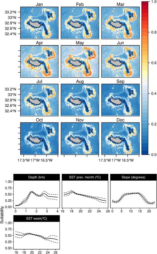
Fernandez et al.                                                                                          Cetaceans’ Distributions in Oceanic Islands

INTRODUCTION                                                               host populations with some degree of residency, such as the
                                                                           short-finned pilot whale (Globicephala macrorhynchus) or the
While the construction of species distributional estimates is              bottlenose dolphin (Tursiops truncatus) (Alves et al., 2013b;
a crucial topic to conserve, protect, manage and monitor                   Dinis et al., 2016a). Other deep-diving cetacean species, such
biodiversity (Rodríguez et al., 2007), it stills remains a challenge       as the sperm whale (Physeter macrocephalus) and Blainville’s
to obtain accurate and reliable products to ensure practical               beaked whale (Mesoplodon densirostris), are among the most
management actions (Araújo et al., 2019). One of the main                  sighted species by commercial whale watching companies with
tools used for these purposes are ecological miche models                  some periodicity.
(ENMs). A class of methods that use occurrence data together                  Moreover, baleen whales occur frequently in the archipelago,
with environmental data to make a correlative model of                     especially the Bryde’s whale (Balaenoptera edeni), with a
the environmental conditions that meet a species’ ecological               relatively high occurrence rate but with a very high interannual
requirements and predict the relative suitability of habitat               variation (Alves et al., 2018). Recent studies revealed cetacean
(Warren and Seifert, 2011). Challenges are even more significant           interconnectivity among neighboring archipelagos, such as the
when estimating species distributions in the marine environment,           Canaries and the Azores, with re-sightings of individuals
where there are many factors to take into account, such as the             from several species among the three archipelagos (e.g.,
species mobility and habitat dynamism (Redfern et al., 2006;               Alves et al., 2019; Dinis et al., 2021). Additionally, Madeira
Fernandez et al., 2017), or the difficulties of sampling at oceanic        constitutes an area of interest for several (at least ten) cetacean
environments, primarily when referring to cetacean populations             species due to being used for traveling, feeding, resting,
(Tyne et al., 2016).                                                       socializing and calving (Alves et al., 2018). However, despite its
    Lately, several studies found that non-traditional data sources        ecological importance, up to date, there are no reliable spatio-
(such as opportunistic or citizen science data; e.g., Catlin-              temporal distributional estimates for any of the cetacean species
Groves, 2012; Embling et al., 2015) can be a cost-effective                present in the area.
solution to overcome some of the challenges mentioned,                        In this study, we provide, for the first time, a fine-scale
allowing to produce relatively accurate cetacean abundance and             spatio-temporal approach to obtain distributional estimates of
distributional estimates (e.g., Fernandez et al., 2018; Robbins            cetaceans around the Madeira archipelago. Having a better
et al., 2019). When studying species in dynamic habitats,                  knowledge of the species suitability throughout the year
opportunistic surveys (and citizen science) can have many                  is critical for their conservation through maritime spatial
advantages over traditional methods. Formal and dedicated                  planning and management of human activities. We built
surveys provide poor coverage in time because of financial and             niche models for the ten most sighted cetacean species
logistic constraints, meaning that they cannot capture long-term           in Madeira, using two different datasets of environmental
variation in species distributions and occurrence.                         variables with different temporal and spatial resolutions.
    Oceanic islands are a key actor on pelagic habitats,                   Models were iterated and selected using several state-of-the-art
congregating biodiversity in their vicinity, primarily due to the          evaluation techniques.
“island-mass effect” (Doty and Oguri, 1956) or “island stirring”
(Mann and Lazier, 1991), which is the topographic disturbance of
oceanic flow by an island and its effects on the marine ecosystem.         MATERIALS AND METHODS
Several oceanographic features, such as wakes and eddies or
vortices (e.g., Aristegui et al., 1994; Caldeira et al., 2002), are        Study Area and Data Collection
originated due to the presence of islands and have a direct effect         The Madeira archipelago is in the NE Atlantic (33◦ N, 17◦ W)
on the local and regional productivity (Barton et al., 2000). Due          and is mainly influenced by a branch of the Gulf Stream, the
to their dynamic nature, their effects on marine species are not           Azores Current system. Caldeira et al. (2002) suggested that the
well understood.                                                           archipelago’s latitude might be the subtropical front, where cold-
    Cetaceans are marine mammals in the order Cetacea, which               temperate waters from the north meet warm tropical waters from
includes whales, dolphins, and porpoises. They have a strong               the south. The island mass effect of the archipelago is easily
influence on the marine ecosystems: as consumers of fish                   noticeable from satellite imagery, with wakes being formed on
and invertebrates, as prey to other predators, as reservoirs               leeward areas and lee eddies spinning of both flanks of Madeira
of carbon, as vertical and horizontal vectors for nutrients                Island. Moreover, upwelling was detected near the island’s coasts,
and as detrital sources of energy and habitat in the deep-                 with the region between Madeira and Desertas Islands being
sea (Roman et al., 2014). Whales and dolphins are essential                particularly dynamic (Caldeira et al., 2002).
to ensure the correct functioning of the marine ecosystems                     Cetacean occurrences were collected in an opportunistically
worldwide, with a vital role in the biogeochemical cycles at               way on-board commercial whale-watching vessels departing
biome and Earth system scale (Albouy et al., 2020; Norris et al.,          from two harbors (Calheta and Funchal) separated over 30 km
2020). A high diversity of cetaceans (∼30 species) has been                on the South Coast of Madeira Island (Figure 1). The
recorded in the Madeira Archipelago (NE Atlantic), including               occurrences were collected by three operators (see section
species featured in the Red List of the International Union for            “Acknowledgments”) during their regular touristic trips from
Conservation of Nature as Endangered, Vulnerable, and Data                 January 2003 until December 2018, with a total of 3,138 days
Deficient (Freitas et al., 2012; Alves et al., 2018). These waters         sampled. Experienced observers from the companies collected

Frontiers in Marine Science | www.frontiersin.org                      2                                       July 2021 | Volume 8 | Article 688248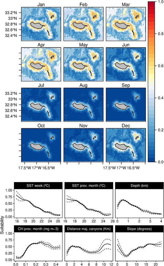
Fernandez et al.                                                                                                        Cetaceans’ Distributions in Oceanic Islands

  FIGURE 1 | Cetacean sightings for 23 species (n = 8,607) pooled together, collected by the commercial whale watching companies departing from Funchal and
  Calheta in Madeira Island (Portugal) from 2003 until 2018.

TABLE 1 | Number of sightings for the 10 most sighted species (out of 23) by             in space and time, which creates autocorrelation problems in
commercial whale watching companies from 2003 until 2018 used in
                                                                                         contiguous grids. Therefore, a filtering approach was applied to
the present study (n = 8,607).
                                                                                         remove potentially related sightings. A spatial thinning procedure
Species                                                                        N         was applied to all the sightings for both temporal groupings (1-
                                                                                         and 8-days), using the spThin R package (Aiello-Lammens et al.,
Atlantic Spotted dolphin (Stenella frontalis)                              3040
                                                                                         2015). Different sizes of the exclusion radius were tested (2, 4,
Bottlenose dolphin (Tursiops truncatus)                                    2733
                                                                                         and 6 km), selecting at the end a value of 2 km, which was
Short-beaked common dolphin (Delphinus delphis)                            1936
                                                                                         the best compromise to reduce related sightings and still keep
Short-finned pilot whale (Globicephala macrorhynchus)                      1503
                                                                                         a good amount of observations. This agrees with the relatively
Bryde’s whale (Balaenoptera edeni)                                             931
                                                                                         small size of the sampled area (around 2,100 km2 ) by the whale-
Sperm whale (Physeter macrocephalus)                                           554
                                                                                         watching boats. Furthermore, during the modeling analysis,
Striped dolphin (Stenella coeruleoalba)                                        292
                                                                                         occurrences were also resampled to one occurrence per pixel for
Blainville’s beaked whale (Mesoplodon densitrostris)                           144
                                                                                         each temporal grouping.
Fin whale (Balaenoptera physalus)                                              130
                                                                                            Due to the sampling effort’s opportunistic nature, we applied
Rough-toothed dolphin (Steno bredanensis)                                      81
                                                                                         a Minimum Sampled Area (MSA) approach, as Fernandez et al.
                                                                                         (2017) used. All the sightings for each specific temporal scale
                                                                                         were pooled together using a Minimum Convex Polygon, adding
location and species identification of each encounter. We applied                        a 2 km buffer. Grids intersecting the polygon were taken as
a database filtering and cleaning to remove duplicate observations                       potentially sampled areas, therefore classified as background.
and incorrect GPS points clearly outside of the study area                               The amount of effort per temporal unit (day or 8-days) was
(or on land). A total of 8,607 sightings from 23 different                               considered using the number of sea trips performed on a
species were selected during this period, from which the ten                             specific period. For each analysis, random background datasets
most sighted species were used in the present study (Table 1).                           (n = 10,000) were created, using the effort as a weighting factor.
Detailed methodological procedures on the data collection on-
board commercial whale-watching vessels are given in Alves et al.
                                                                                         Environmental Variables
(2018).
                                                                                         A set of 19 environmental variables were used to calibrate
                                                                                         the models (Table 2). Six terrain variables (depth, slope, and
Occurrences and Background Data                                                          distance to the 1,000 m bathymetric lines, valley depth, distance
All occurrences records were projected onto 2 and 8 km grids                             to canyon-like features, and distance to major canyons) were
to match the resolution of the two environmental datasets.                               derived from a digital elevation model (DEM) using the
Observations data collected on whale-watching operations might                           bathymetric dataset from the Instituto Hidrográfico of Portugal
have a different source of biases due to the nature of the touristic                     and interpolated using QGIS 3.1 at a resolution of 1 km.
activity. For example, it is not unusual that the same group of                          Physical features, such as the depth and the slope, can directly
animals is visited more than once in a very similar location, both                       influence the distribution of cetaceans (e.g., Moore et al., 2000;

Frontiers in Marine Science | www.frontiersin.org                                    3                                       July 2021 | Volume 8 | Article 688248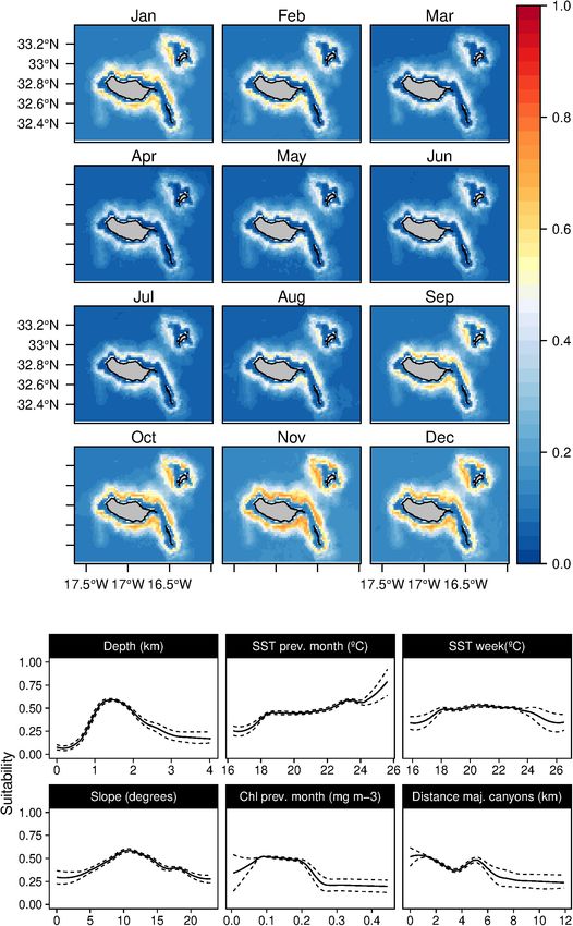
Fernandez et al.                                                                                        Cetaceans’ Distributions in Oceanic Islands

Azzellino et al., 2008). Depth was directly read from the                keeping all the canyon-related variables (see the final variables
DEM; slope and distances to the 1,000 m bathymetric lines                selected for the analysis in Table 2).
were calculated using QGIS 3.1. Moreover, other morphological                Two different sets of environmental layers were constructed.
features, such as canyons, can play an essential role in cetacean        The first assemblage (the daily set) aimed to detect the
distributions. Canyons and other similar features can affect             effect of dynamic variables at a coarse spatial resolution
cetacean abundance patterns due to a series of physical features         (7.8 km) and included a set of nine oceanographic variables
that enhance primary productivity and convert it to potential            at different depths with a daily resolution. The cumulative
prey biomass (Moors-Murphy, 2014). These effects are even                effect of variables (temperature and Chl-a) was measured as
more noticeable when dealing with deep-diving cetacean species,          the mean values for the 30 days previous to the sightings.
which might directly rely on these areas for feeding purposes            The second group of layers (the 8-day set) aimed to
(Breen et al., 2020).                                                    detect the influence of topographic features on a fine-
    We calculated a series of morphological variables to include         scale resolution (2 km), including a set of 4 oceanographic
the effects of morphological features as prey aggregation areas          variables with an 8-day (Table 2). The 30-day mean values of
into the models. The valley depth refers to the vertical distance        temperature and Chl-a were included to test for those variables’
to a channel network base level; it was calculated using the             cumulative effects.
QGIS module “Relative Heights and Slope Positions” based
on Boehner and Selige (2006). The canyon-like features were              Modeling Building and Evaluation
calculated using the topographic position index (TPI), which             Due to the opportunistic nature of the data used in this study,
measures where a point is in the overall landscape/seascape to           without real absences, we used a presence-background algorithm
identify features such as ridges, canyons, or midslopes (Wright          MAXENT (Phillips et al., 2006) to infer the ecological niche
and Heyman, 2008). We computed the TPI with the SAGA GIS1                model of the selected species.
implementation (based on Guisan et al., 1999; Weiss, 2001),                  The kuenm package (Cobos et al., 2019a) in R was used
using a radius of 3,000 m. We selected features corresponding            to select the most important variables, build and evaluate the
to V-shape river valleys and deep narrow canyons (Weiss, 2001).          MAXENT models. Data was introduced using the sightings
We applied a spatial filter (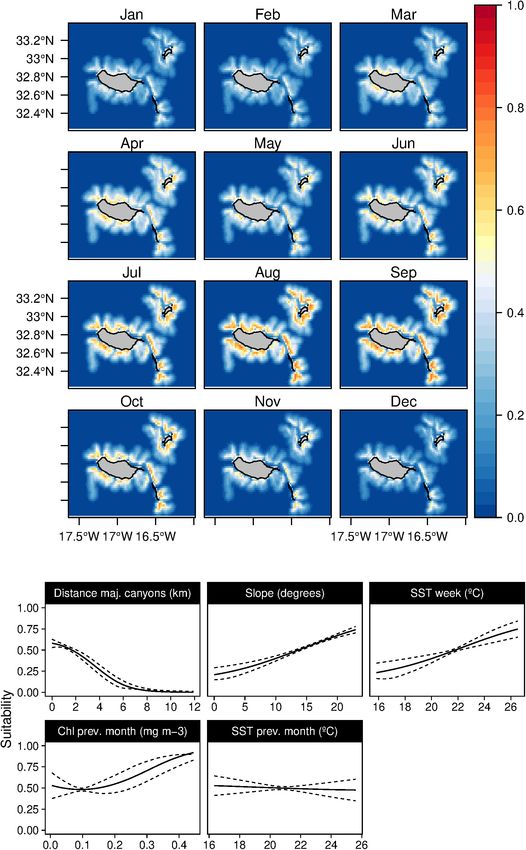
Fernandez et al. Cetaceans’ Distributions in Oceanic Islands
TABLE 2 | Variables used to construct the two different assemblages of layers for the present analysis: the (1) “D” set with a spatial resolution of 7.8 km and a temporal
resolution of 1 day, and the (2) “8-D” set, with a spatial resolution of 2 km and a temporal resolution of 8-days and 1 month.
ACR Variables D set 8-D set UNITS Product source/ID
√ √
DEPTH Depth m Resampled from Instituto Hidrográfico
√ √ ◦
SLOPE Bottom slope Calculated and resampled from Instituto Hidrográfico
√
VALLEY_DEPTH Vertical distance to a channel network m Calculated and resampled from Instituto Hidrográfico
base level
√
D_M_CANYONS Distance to major canyon like features Km Calculated and resampled from Instituto Hidrográfico
√
D_CANYONS Distance to canyon like features Km Calculated and resampled from Instituto Hidrográfico
√ ◦C
SST Sea surface temperature GHRSST Level 4 MUR Global Foundation Sea Surface
Temperature Analysis (v4.1)
√ ◦C
TEMP_0.5 Sea water potential temperature at Atlantic-Iberian Biscay Irish-Ocean Physic Reanalysis
0.5 m product: IBI_REANALYSIS_PHYS_005_001
√ ◦C
TEMP_100 Sea water potential temperature at Atlantic-Iberian Biscay Irish-Ocean Physic Reanalysis
108 m product: IBI_REANALYSIS_PHYS_005_001
√ ◦C
TEMP_700 Sea water potential temperature at Atlantic-Iberian Biscay Irish-Ocean Physic Reanalysis
773 m product: IBI_REANALYSIS_PHYS_005_001
√ ◦C
TEMP_PR_0.5 Sea water potential temperature at Atlantic-Iberian Biscay Irish-Ocean Physic Reanalysis
0.5 m of the previous month product: IBI_REANALYSIS_PHYS_005_001
√ ◦C
TEMP_PR_100 Sea water potential temperature at Atlantic-Iberian Biscay Irish-Ocean Physic Reanalysis
108 m of the previous month product: IBI_REANALYSIS_PHYS_005_001
√ ◦C
TEMP_PR_700 Sea water potential temperature at Atlantic-Iberian Biscay Irish-Ocean Physic Reanalysis
773 m of the previous month product: IBI_REANALYSIS_PHYS_005_001
√
SAL_S Sea water salinity at 0.5 m ppt Atlantic-Iberian Biscay Irish-Ocean Physic Reanalysis
product: IBI_REANALYSIS_PHYS_005_001
√
MIXED_LAYER Mix layer depth m Atlantic-Iberian Biscay Irish-Ocean Physic Reanalysis
product: IBI_REANALYSIS_PHYS_005_001
√
SSH Sea surface height Cm Atlantic-Iberian Biscay Irish-Ocean Physic Reanalysis
product: IBI_REANALYSIS_PHYS_005_001
√ √
CHL Chlorophyll-a concentration in sea mg·m−3 North Atlantic Chlorophyll Concentration from Satellite
water observations reprocessed L4 (ESA-CCI) product:
OCEANCOLOUR_ATL_CHL_L4_REP_OBSERVATIONS_
009_098
√ √
LUNAR_IL Lunar illumination Lux R “lunar” package
√ √
CHL_PR Chlorophyll-a concentration in sea mg·m−3 North Atlantic Chlorophyll Concentration from Satellite
water of the previous month observations reprocessed L4 (ESA-CCI) product:
OCEANCOLOUR_ATL_CHL_L4_REP_OBSERVATIONS_
009_091
√ ◦C
SST_PR Sea surface temperature of the GHRSST Level 4 MUR Global Foundation Sea Surface
previous month Temperature Analysis (v4.1)
both overfitting and underfitting when comparing it to a classical the evaluation, we used the expert-based omission criterion as a
heuristic method (Cobos et al., 2019b). complementary validation method.
The best models were selected by the kuenm process, only Projections of the models were made for each combination
in one case (fin whales on the daily scenario); we did not select of year/month from 2003 to 2018 using a clamping approach to
the best option given by kuenm, but one of the other potential avoid extrapolations to areas outside of the range of the training
candidates selected during the process. In this case, the best conditions (Merow et al., 2013). Finally, the mean suitability
model was slightly overfitted to coastal areas due to the relatively values and standard deviation for all months through all years
low number of observations for the species and the bias associated were calculated.
with the whale-wacthing activity. Therefore, we selected a model
with no restrictions on the Depth variable, as we know that fin
whales are also frequently sighted offshore. RESULTS
To select between the two different environmental datasets
tested (with different temporal and spatial resolution), we used Model Performance
an expert-based omission criterion (areas/time being classified as A total of 87,300 model solutions were generated for the 8-
unsuitable when they are not). Experts evaluation and knowledge day dataset, and 300,300 were generated for the daily data. The
were based on empirical observations of the target species around best results were selected according to their relative predictive
the archipelago in different periods outside the study area. and explanatory capabilities. According to expert knowledge
However, as these datasets were not available at the moment of criteria, models built using the 8-day dataset, with a higher
Frontiers in Marine Science | www.frontiersin.org 5 July 2021 | Volume 8 | Article 688248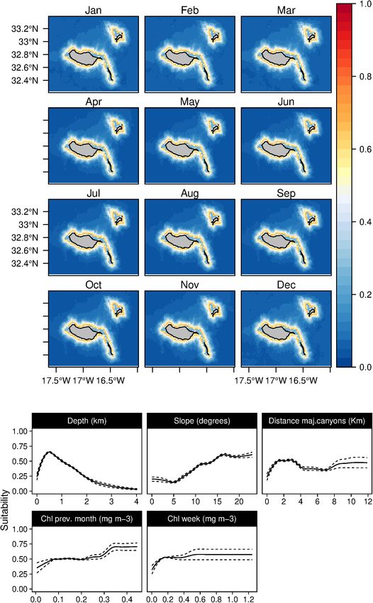
Fernandez et al. Cetaceans’ Distributions in Oceanic Islands
TABLE 3 | Eight-days models regularization multiplier (REG.), feature classes (linear = l, quadratic = q, product = p, threshold = t, and hinge = h), omission rate at 5%
(OR 5%), area under the curve (AUC), and variables selected (with its contribution) for each species.
Species REG. FEAT. OR 5% AUC Vars selected
Globicephala macrorhynchus* 1.5 lqpt 0.048 0.75 Depth (62.5%).
SST previous month (17%).
SST week (7.4%).
Slope (7.3%).
Chl-a previous month (3.9%).
Distance to major canyons (2%).
Physeter macrocephalus* 1.5 lqpt 0.045 0.73 Depth (59.3%).
SST week (12.4%).
Valley depth (11.1%).
Slope (6.3%).
Distance to canyons (5.9%).
Distance to major canyons (4.9%).
Mesoplodon densirostris* 1.5 lqp 0.032 0.73 Distance to major canyons (36.3%).
Slope (31.8%).
SST week (20.5%).
Chl-a previous month (7%).
SST previous month (4.5%).
Stenella frontalis* 2 lqpth 0.044 0.7 Depth (46.4%).
SST previous month (23.3%).
Chl-a week (17.9%).
SST week (10.5%).
Chl-a previous month (2%).
Tursiops truncatus* 1.5 lqpt 0.046 0.73 Depth (73.4%).
Slope (19.6%).
Distance to major Canyons (5%).
Chl-a previous month (1%).
Chl-a week (1%).
Delphinus delphis* 1 lqpt 0.048 0.81 SST week (30.9%).
Chl-a previous month (20.8%).
Depth (17%).
SST previous month (14.3%).
Slope (12.2%).
Distance to major canyons (4.8%).
Stenella coeruleoalba* 1.5 lqpt 0.048 0.80 Depth (59.5%).
SST previous month (19.4%).
Slope (15.5%).
SST week (5.6%).
Steno bredanensis* 1 lqpt 0 0.90 SST week (57.1%).
Slope (23.5%).
Lunar illumination (13.9%).
Distance to major canyons (5.4%).
Balaenoptera physalus 1.5 lqpt 0.038 0.88 Chl-a week (41.4%).
SST previous month (38.1%).
Lunar illumination (12.2%).
Depth (8.3%).
Balaenoptera edeni 1 lq 0.044 0.75 SST week (50.5%).
Depth (43.2%).
Chl-a week (6.3%).
Variables are sorted by percent contribution to the final model. Models marked with an asterisk are the ones selected as “Best.”
spatial resolution and more topographic-based variables, had a (ii) delphinids (bottlenose dolphins, rough-toothed dolphins,
better predictive performance. For 8 of the 10 species considered Atlantic spotted dolphins, short-beaked common dolphins and
in the present study (G. macrorhyncus, P. macrocephalus, M. striped dolphins), and (iii) balaenopterids (fin whales and
densirostris, S. frontalis, T. truncatus, D. delphis, S. coeruleoalba, Bryde’s whales).
and S. bredanensis), the 8-day scenario produced better results
(Table 3). Only two species (B. edeni and B. physalus) produced Deep-Divers
better estimates when using the daily dataset. The results are All the deep-diving species higher suitability values were
presented per functional ecological groups: (i) deep-divers (short- related to the bathymetry or other topographic variables.
finned pilot whales, sperm whales and Blainville’s beaked whale), The short-finned pilot whales (G. macrorhynchus) suitable
Frontiers in Marine Science | www.frontiersin.org 6 July 2021 | Volume 8 | Article 688248
Fernandez et al. Cetaceans’ Distributions in Oceanic Islands
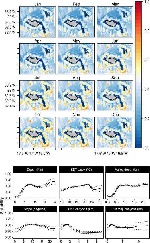
areas were related with depths between 1,000 and 2,000 m values. Relatively high suitability values for the species were
with intermediate slope values and a slight preference for found from July to October, with high standard deviation values
regions closer to major canyons (Figure 2). The SST played in June and November (Supplementary Figure 5).
a relevant role in the species niche, with a preference for In both of the modeling approaches used in this study,
warm waters (18–24◦ C) and low Chl-a values. The daily only one topographic variable was identified as an important
analysis results showed an influence of the shallow mixed predictor for the Atlantic spotted dolphins (S. frontalis), the
layer in the suitability. Models projections suggest a patched bathymetry (Tables 3, 4). The species showed a preference for
temporal and spatial distribution of the species, with highly relatively deep-waters around the 1,000 m isoline. Moreover, both
suitable areas found at the South-east and North of Madeira. during the 8-day and in the previous month, the temperature
Seasonal variability was found, with lower suitability values was selected as the models’ relevant variables. Atlantic spotted
from March to July. However, high standard deviation values dolphins niche was related with temperate/warm waters (over
were found in March and April (Supplementary Figure 1). 18◦ C) with very low productivity values (Figure 7), leading to
Lastly, the daily models showed a subtle influence of the lunar higher suitability values from June until October. However, high
illumination on the species, with higher suitability indexes standard deviation values are found between February and May
with lower values. (Supplementary Figure 6), which denotes the high variability of
Sperm whales (P. macrocephalus) habitat was related with the suitability indexes in those months.
waters deeper than 1 km, with an intermediate slope and closer to In contrast, the short-beaked common dolphins (D. delphis)
any type of canyons (Figure 3). The analysis suggested a relation presented a strong relation with lower values of SST (both in
with areas with low valley depths and close to canyons on mid- the weekly and previous month) along with high values of Chl-
slope areas. Only one oceanographic variable was found relevant a during the previous month (Figure 8). This delphinid niche
for the model selected (the SST), denoting a slight preference was also related to relatively shallow waters, moderate to high
of the species for warmer waters. Low standard deviation values slope regions, and areas closer to major canyons. Moreover, the
of suitability were found (Supplementary Figure 2) for all the daily model showed an influence of the mixed layer depth on
months. the species niche. Common dolphins had higher suitability values
Blainville’s beaked whales (M. densirostris) models showed a in winter and spring (from December to June), with moderate
significant contribution of the major canyons, slope, and SST, standard deviation values in June (Supplementary Figure 7).
with a total contribution of 88.6% on the model construction The striped dolphins (S. coeruleoalba) were predominantly
(Table 3). The species was related to areas with major related to deep waters regions (over 1,000 m) and moderate
canyons, with high slope values and a positive correlation with slope values (Figure 9), alongside a preference for temperate
warm waters (Figure 4). Moreover, a marginal effect of the waters (around 19–20◦ C). While the suitability values obtained
Chl-a and SST on the previous month was also observed. indicate a year-round presence of these delphinids in the
This species showed a patchy distribution primarily in the archipelago, higher suitability values were found from spring
vicinity of canyons and a temporal preference for summer to early summer, with very low standard deviation values
and early autumn. Nonetheless, the standard deviation maps (Supplementary Figure 8).
(Supplementary Figure 3) show relatively high values from
January to April. Balaenopterids
Oceanographic variables were constantly selected as the most
Delphinids influential variables for the baleen whales’ ecological niche
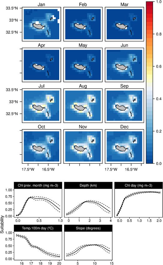
The suitability for bottlenose dolphins (T. truncatus) was found in the present study. The fin whales suitability (B. physalus)
to be primarily related to the bathymetry, slope, and distance was influenced mainly by moderate values of Chl-a in the
to the major canyons, contributing up to 98% to the selected previous month, together with high daily Chl-a values and low
model (Table 3). The species suitability was positively linked to daily values of temperature in 100 m depth. Topographically,
relatively shallow waters with high slope values and somehow the species niche was related to intermediate bathymetry
close to major canyons. Even if marginal, there is also a (with a peak at 2,000 m) and mid-slope values (Figure 10).
preference for waters with high Chl-a values (Figure 5). These Suitability maps exhibited elevated values from February to May,
outcomes produced a generalist distribution of the species on with high standard deviation values from February to August
Madeira’s coastal areas with almost no temporal variability, (Supplementary Figure 9).
also reflected on the low values of standard deviation maps Conversely, very low values of Chl-a during the previous
(Supplementary Figure 4). month were more related to the Bryde’s whales (B. edeni) niche,
The weekly SST was found to be the most influential together with sea surface temperatures in the previous month
factor (Figure 6) determining the rough-toothed dolphins between 20 and 24◦ C (Figure 11). This species’ results also
(S. bredanensis) niche, being linked to warmer waters (above indicated a relation with waters around 1,000 m depth and
20◦ C). The daily scenario models also showed a relation between a positive correlation with the warmer daily temperature at
warm waters and shallow mixed layer depth. Topographically, 100 m. Suitability values for Bryde’s whales were relatively low,
the niche was linked with mid and high slope values in the with a slight increase from June to January; however, high
proximity of major canyons. The results revealed a relation standard deviation values were found from June to November
between rough-toothed dolphin niche and low lunar illumination (Supplementary Figure 10).
Frontiers in Marine Science | www.frontiersin.org 7 July 2021 | Volume 8 | Article 688248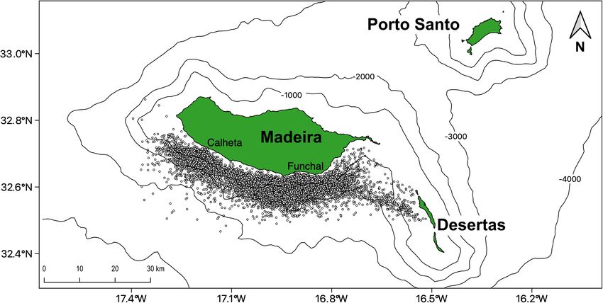
Fernandez et al.                                                                                                          Cetaceans’ Distributions in Oceanic Islands

  FIGURE 2 | Mean monthly suitability maps (above) and smoothed response curves with standard deviation (below) in the Madeira archipelago for Globicephala
  macrorhynchus for the “8-days” models. In the maps, red represents more suitable and blue less suitable. Responses curves are ordered by percent contribution of
  the environmental variables.

DISCUSSION                                                                           indicates good overall predictive performance. This reinforces
                                                                                     the potential of opportunistically collected datasets to produce
The long-term opportunistic dataset used in this study provided                      reliable estimates of habitat suitability, as Henckel et al.
an excellent opportunity to build reliable ecological niche models                   (2020) found recently.
with various environmental conditions. Even if the AUC values                            While a series of techniques to reduce overfitting and select
alone might not be the best model performance indicator                              the best models were applied (e.g., AICc index for model
(Lobo et al., 2008), all selected models ranged between 0.7                          selection), few coincidental relationships between suitability
and 0.9, which, together with the low omission rate values,                          predictions and environmental variables might still be present.

Frontiers in Marine Science | www.frontiersin.org                                8                                              July 2021 | Volume 8 | Article 688248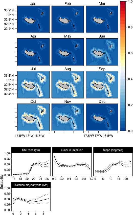
Fernandez et al.                                                                                                          Cetaceans’ Distributions in Oceanic Islands

  FIGURE 3 | Mean monthly suitability maps (above) and smoothed response curves with standard deviation (below) in the Madeira archipelago for Physeter
  macrocephalus for the “8-days” models. In the maps, red represents more suitable and blue less suitable. Responses curves are ordered by percent contribution of
  the environmental variables.

Some of the relations found in the response curves (such                             techniques implemented assure good predictive performance for
as the high suitability predictions on low slope values found                        the models built.
for the common dolphins; Figure 8) might look odd and                                    Despite the small area where data was collected (limited
spurious, affecting the explanatory power. Explanatory power                         mainly to the South coast of Madeira and West of Desertas
and predictive accuracy are different qualities; a model will                        islands), experts confirmed that extrapolated areas agree with
possess some level of each (Shmueli, 2010). Therefore, even if                       their experience. However, using a reduced area to collect
few coincidental relationships might be present, the validation                      training data might result in a truncated response curve

Frontiers in Marine Science | www.frontiersin.org                                9                                              July 2021 | Volume 8 | Article 688248
Fernandez et al.                                                                                                            Cetaceans’ Distributions in Oceanic Islands

  FIGURE 4 | Mean monthly suitability maps (above) and smoothed response curves with standard deviation (below) in the Madeira archipelago for Mesoplodon
  densirostris for the “8-days” models. In the maps, red represents more suitable and blue less suitable. Responses curves are ordered by percent contribution of the
  environmental variables.

for some variables, missing fundamental environmental                                  as the sperm whale, the short-finned pilot whale, or the
values to fully describe the niche (Thuiller et al., 2004;                             bottlenose dolphin). The Maxent clamping implementation
Williams and Jackson, 2007). This could be the case,                                   mitigates this issue (Phillips et al., 2006; Anderson and
especially for those more bottom-related species (such                                 Raza, 2010); however, preferably, a wider sampling area with

Frontiers in Marine Science | www.frontiersin.org                                 10                                              July 2021 | Volume 8 | Article 688248
Fernandez et al.                                                                                                            Cetaceans’ Distributions in Oceanic Islands

  FIGURE 5 | Mean monthly suitability maps (above) and smoothed response curves with standard deviation (below) in the Madeira archipelago for Tursiops
  truncatus for the “8-days” models. In the maps, red represents more suitable and blue less suitable. Responses curves are ordered by percent contribution of the
  environmental variables.

different topographic characteristics would be the best way to                         in the three dimensions. However, its informative potential was
overcome this concern.                                                                 primarily reduced due to the dataset’s coarse spatial resolution
   The daily models added some relevant information on species                         and the use of a broad-scale circulation oceanographic algorithm.
niches, as it considers a broader range of oceanographic variables                     Using models with a finer spatial resolution and including

Frontiers in Marine Science | www.frontiersin.org                                 11                                              July 2021 | Volume 8 | Article 688248
Fernandez et al.                                                                                                           Cetaceans’ Distributions in Oceanic Islands

  FIGURE 6 | Mean monthly suitability maps (above) and smoothed response curves with standard deviation (below) in the Madeira archipelago for Steno
  bredanensis for the “8-days” models. In the maps, red represents more suitable and blue less suitable. Responses curves are ordered by percent contribution of the
  environmental variables.

atmosphere-ocean interactions could improve the results, giving                       Species Ecological Findings
more insights on fine-scale features that can influence cetacean                      Deep-Divers
distributions. This fact is especially relevant when considering                      The three deep-diving species (G. macrorhynchus,
the fine-scale structures generated by the island in the archipelago                  P. macrocephalus, and M. densirostris) showed differentiated
(Caldeira et al., 2002).                                                              niches, both in the spatial and temporal dimensions. The

Frontiers in Marine Science | www.frontiersin.org                                12                                              July 2021 | Volume 8 | Article 688248
Fernandez et al. Cetaceans’ Distributions in Oceanic Islands
TABLE 4 | Daily models regularization multiplier (REG.), feature classes (linear = l, quadratic = q, product = p, threshold = t, and hinge = h), omission rate at 5% (OR 5%),
area under the curve (AUC), and variables selected (with its contribution) for each species.
Species REG. FEAT. OR 5% AUC Vars selected
Globicephala macrorhynchus 1 lqpt 0.044 0.74 Depth (62.7%).
Slope (19.4%).
Mixed layer depth (7.8%).
SSH (7.5%).
Lunar illumination (2.5%).
Physeter macrocephalus 1.5 lqp 0.047 0.65 Depth (40%).
Slope (34.8%).
Temp. at 0.5 m previous month (22%).
Temp. at 700 m daily (3.2%).
Mesoplodon densirostris 1.5 lqpth 0.034 0.73 Slope (55.5%).
Temp. at 0.5 m daily (30%).
Temp. at 0.5 m previous month (8%).
Chl-a previous month (6.4%).
Stenella frontalis 1.5 lqpth 0.047 0.74 Depth (48.9%).
Temp. at 0.5 m daily (20.6%).
Temp. at 0.5 m previous month (19.1%).
Temp. at 100 m previous month (9.7%).
Temp. at 100 m daily (1.8%).
Tursiops truncatus 1 lqpt 0.05 0.68 Slope (60.3%).
Depth (25.7%).
Temp. at 100 m previous month (9.7%).
Temp. at 0.5 m previous month (6.7%).
Delphinus delphis 1.5 lqpt 0.047 0.77 Temp. at 0.5 m previous month (43.2%).
Chl-a previous month (24.6%).
Slope (23.4%).
Mixed layer depth (6.4%).
Depth (2.5%).
Stenella coeruleoalba 2 lqpth 0.032 0.76 Depth (52.7%).
Temp. at 0.5 m previous month (23.6%).
Slope (10.3%).
Mixed layer depth (9.6%).
SSH (3.8%).
Steno bredanensis 2 lqpth 0 0.86 Temp. at 0.5 m previous month (48%).
Mixed layer depth (31.2%).
Slope (19.3%).
Temp. at 100 m previous month (1.5%).
Balaenoptera physalus* 2 lqpt 0.038 0.85 Chl-a previous month (52%).
Depth (20.5%).
Chl-a daily (14.2%).
Temp. at 100 m daily (9.4%).
Slope (3.9%).
Balaenoptera edeni* 1 lqpt 0.049 0.85 Temp. at 0.5 m previous month (33.5%).
Chl-a previous month (25.6%).
Depth (19.7%).
Temp. at 100 m daily (11%).
SSH (10.2%).
Variables are sorted by percent contribution to the final model. Models marked with an asterisk are the ones selected as “Best.”
short-finned pilot whales’ ecological niche was clearly described temporal occurrence pattern for the species in the archipelago
by a preference for warmer waters (over 18◦ C) and low/moderate seems to be shaped by the SST and Chl-a, with resultant higher
chlorophyll values. The species was found to be related to waters suitability values in late-summer/autumn and winter (Figure 2).
slightly deeper than 1,000 m, which agrees with the findings These findings are in accordance with the known species’
on the diving behavior for the species by Soto et al. (2008) in temporal occurrence and might be related to some of the inter-
the Canary Islands and Alves et al. (2013a) in Madeira, with archipelagic movements registered by Alves et al. (2019). Some
dives between 500 and 1,000 m. While major canyons played a animals might travel to other areas (such as the Azores or the
role in the distribution of pilot whales, higher suitability values Canary Islands) using oceanographic features, like the long-lived
were found mostly related to moderate slopes. This agrees with eddies in the Macaronesian region described by Sangrà et al.
Thorne et al. (2017) findings, where canyons and the shelf-break (2009) and Caldeira (2019), a behavior already observed for
zones were found to be suitable habitat for tracked animals. The this species by Thorne et al. (2017) when following the Gulf
Frontiers in Marine Science | www.frontiersin.org 13 July 2021 | Volume 8 | Article 688248Fernandez et al. Cetaceans’ Distributions in Oceanic Islands FIGURE 7 | Mean monthly suitability maps (above) and smoothed response curves with standard deviation (below) in the Madeira archipelago for Stenella frontalis for the “8-days” models. In the maps, red represents more suitable and blue less suitable. Responses curves are ordered by percent contribution of the environmental variables. stream meanders off the Atlantic Coast of the United States. These findings might be related to the subtle influence of the Furthermore, Owen et al. (2019) recently found an influence lunar illumination we found in the daily models (Table 3); results of the lunar moon on the behavior and distribution of pilot indicated that suitability around the island was lower with higher whales in Hawaii, with a displacement toward offshore waters, lunar illumination. Nevertheless, other approaches would be together with deeper and longer dives during the full moon. needed to understand this potential effect better. Frontiers in Marine Science | www.frontiersin.org 14 July 2021 | Volume 8 | Article 688248
Fernandez et al.                                                                                                            Cetaceans’ Distributions in Oceanic Islands

  FIGURE 8 | Mean monthly suitability maps (above) and smoothed response curves with standard deviation (below) in the Madeira archipelago for Delphinus
  delphis for the “8-days” models. In the maps, red represents more suitable and blue less suitable. Responses curves are ordered by percent contribution of the
  environmental variables.

   Sperm whales are known to be a cosmopolitan species                                 for waters deeper than 1 km (but not restricted to a specific range)
(Jefferson et al., 2011). Even if mostly feeding on cephalopods,                       in the proximity of submarine canyons areas. While the species
they can be considered generalist foragers, consuming a wide                           seems to be present in the archipelago throughout the year, there
variety of prey (e.g., Clarke, 1980; Evans and Hindell, 2004).                         is an apparent increase in suitability from June to November,
Our results showed a broader niche of the species on the spatial                       linked to SST, with a peak around 23◦ C, similar to other areas,
dimension than the short-finned pilot whales, with a preference                        such as the Azores (Fernandez et al., 2018). In Madeiran waters,

Frontiers in Marine Science | www.frontiersin.org                                 15                                              July 2021 | Volume 8 | Article 688248
Fernandez et al.                                                                                                            Cetaceans’ Distributions in Oceanic Islands

  FIGURE 9 | Mean monthly suitability maps (above) and smoothed response curves with standard deviation (below) in the Madeira archipelago for Stenella
  coeruleoalba for the “8-days” models. In the maps, red represents more suitable and blue less suitable. Responses curves are ordered by percent contribution of the
  environmental variables.

the group size for the species ranges between 1 and 30 animals,                        groups with offspring in the archipelago might be related with the
with calves present in 25% of the groups (Alves et al., 2018).                         increase of suitability observed from June to December.
Pirotta et al. (2020), found that solitary animals and groups                             Finally, the Blainville beaked whale shows the most restricted
used areas with different characteristics in the Balearic Islands,                     ecological niche of the deep-diving species, mainly being linked
with groups preferring warmer waters. Therefore, the presence of                       to steep relief areas in the vicinity of major canyons (Table 3).

Frontiers in Marine Science | www.frontiersin.org                                 16                                              July 2021 | Volume 8 | Article 688248
Fernandez et al.                                                                                                         Cetaceans’ Distributions in Oceanic Islands

  FIGURE 10 | Mean monthly suitability maps (above) and smoothed response curves with standard deviation (below) in the Madeira archipelago for Balaenoptera
  physalus for the “daily” models. In the maps, red represents more suitable and blue less suitable. Responses curves are ordered by percent contribution of the
  environmental variables.

This results in a very spatially constrained niche in some areas                     the species (Arranz et al., 2011). Finally, the explicit contribution
close to the island’s shoreline, which agrees with the findings in                   of the SST to the models suggests a preference for warm waters,
other regions, such as the Canary Islands (Ritter and Brederlau,                     as suggested by Macleod (2000). All these results lead to relatively
1999) and Hawaii (Schorr et al., 2009). The strong relation found                    good suitability values almost all year round, peaking in summer
with steep areas is probably related to the prey aggregation on                      and early autumn months, which explains the high site fidelity
these specific habitats, representing a reliable food resource for                   patterns previously found by Dinis et al. (2017) around Madeira.

Frontiers in Marine Science | www.frontiersin.org                               17                                             July 2021 | Volume 8 | Article 688248
Fernandez et al.                                                                                                       Cetaceans’ Distributions in Oceanic Islands

  FIGURE 11 | Mean monthly suitability maps (above) and smoothed response curves with standard deviation (below) in the Madeira archipelago for Balaenoptera
  edeni for the “daily” models. In the maps, red represents more suitable and blue less suitable. Responses curves are ordered by percent contribution of the
  environmental variables.

Delphinids                                                                          clear preference for shallow coastal waters (
Fernandez et al.                                                                                            Cetaceans’ Distributions in Oceanic Islands

in the low variability of the suitability values during the year            might be related to the deep-diving foraging behavior previously
(Supplementary Figure 4). Interestingly, we found a marginal                documented in the Azores (Silva et al., 2013). The 8-day analysis
effect of the surface chlorophyll on their distribution, which              also showed an influence of the previous month SST, peaking
could be related to fine-scale effects of primary productivity on           around 18–20◦ C, which agrees with findings by Fernandez et al.
the species distribution, as found for the species in shallow seas          (2018) from the Azores. Conversely, in the present study, the
(Scott et al., 2010).                                                       chlorophyll levels were also relevant (with a preference of values
    While the rough-toothed dolphin was also linked to areas                higher than 0.5 mgm−3 ), which might be a limiting factor for the
with medium or high bottom inclination (usually associated with             species in Madeira. As a result, higher suitability values (and high
islands or seamounts), the temporal distribution for this species           standard deviation) are found mostly during the spring months,
mainly was limited due to a preference for warm waters (over                compared to the Azores, where the species has been recorded
21–22◦ C), such as those on the warm wake present mostly on                 during winter, spring, and summer (Silva et al., 2014). In the
summer months on the South Coast of Madeira (Caldeira et al.,               Azores, the combination of the complex topography with the
2002; Alves et al., 2021).                                                  highly energetic eddy field creates a confluence zone between
    When looking at the small delphinids an interesting pattern             the west and the east North Atlantic (Caldeira and Reis, 2017).
was found, with two species (D. delphis and S. frontalis) with              Additionally, Caldeira (2019) found that the number of long-
differentiated ecological niches. Both species have a similar               lived eddies (lifetime greater than 60 days) generated by the
spatial distribution, with a widespread distribution around the             interaction of the oceanic flow with the islands is much larger
islands, clearly demonstrated by the influence of depth. However,           in the Azores (n = 202) than in Madeira (n = 50). Considering
differences arise when looking at their temporal distribution;              that mesoscale eddies can modulate oceanic productivity in many
the common dolphin was closely related to lower SST values                  ways (Dufois et al., 2016), together with the existence of a
and high chlorophyll concentrations, while the Atlantic spotted             confluence area, might support the extended temporal presence
dolphin preferred warm waters and low chlorophyll values                    of fin whales in the Azores compared to Madeira.
(Figures 7, 8). As a result, higher suitability values were found in            While not much is known, the results presented here agree
winter/spring for the former species and summer/autumn for the              with the Bryde’s whales described literature. The species is known
later species. Au and Perryman (1985) found that in the Eastern             to move through tropical and warm-temperate waters, with a
Tropical Pacific, common dolphins were found to be associated               specific preferred thermal range (Kato and Perrin, 2018). We
with upwelling modified waters, while tropical spotted dolphins             found that higher suitability values mainly were related to warm
(Stenella attenuata) were associated with tropical waters. In               surface waters and low surface chlorophyll concentrations during
the present study, instead of S. attenuata, we have S. frontalis;           the previous months (Figure 11). This agrees with the higher
however, a similar pattern seems to occur, with common dolphins             number of sightings for this species in summer/autumn in the
preferring “cold” waters rich in nutrients and Atlantic spotted             archipelago (Alves et al., 2018). The relatively low suitability
dolphins more associated with warm, and therefore, stratified               values and the high standard deviation we detected could be
areas. This is in agreement with the seasonal regimes found in              caused by the high variability of interannual occurrence rates.
the waters surrounding Madeira, reflected by the ocean static               In the present study, the species was related to a specific SST
stability, with a much better mixed upper ocean in winter and               (between 20 and 24◦ C). Nevertheless, in California, no significant
a more stratified structure present in summer (Alves et al., 2021).         effect of the temperature occurrence pattern was found, with
    Our findings agree with the observations made by Freitas                observations of animals in waters as cold as 15◦ C (Kerosky et al.,
et al. (2004) for Madeira and are in harmony with the niche                 2012). The same authors hypothesize that interannual climate
segregation hypothesis made by Silva et al. (2014) for the Azores.          oscillations and oceanographic indexes (such as the ENSO) could
Nevertheless, it is true that when environmental conditions are             explain some of the variability observed, recognizing that other
suitable for both species, they might occupy the same areas.                environmental variables rather than the SST might influence the
Furthermore, if we also add the high standard deviation values              whales’ movements. Therefore, depending on general circulation
found in the suitability for the Atlantic spotted dolphins, it              patterns, the animals might move to Madeira, to northern
is possible that in some years both species might have high                 latitudes, up to the Azores (Steiner et al., 2008), or could remain
suitability values during some months, especially in spring and             in southern latitudes.
early summer. Finally, the striped dolphin was found to be an
offshore species primarily occurring in deeper waters with a
slight preference for lower temperatures and related to mid-                CONCLUSION
slope areas, agreeing with the findings of Fernandez et al.
(2018) for the Azores.                                                      The distributional estimates presented here are the first attempt
                                                                            to better understand spatial-temporal patterns of cetaceans in
Balaenopterids                                                              the Madeira archipelago. Except for the fin whale, all the
The two balaenopterids considered herein proved to have very                other nine species analyzed in the present study showed a
differentiated niches. The fin whale mainly was related to high             clear relation with specific topographic features, which might
chlorophyll concentrations during the previous month and                    be related to the island-mass effect and associated eddies.
on the same day (Figure 10). The niche was shaped by the                    To better understand how the specific fine-scale island-related
low water temperature preference at 100 m (
Fernandez et al. Cetaceans’ Distributions in Oceanic Islands
recommend using coupled atmospheric-ocean models in future FUNDING
studies. The use of fine-scale accurate data (both in the temporal
and spatial dimension) is crucial to improve dynamic ocean This study was supported by: (i) INTERTAGUA, MAC2/1.1.a/385
management actions in cetaceans, as demonstrated recently by funded by MAC INTERREG 2014-2020, (ii) Oceanic
Hausner et al. (2021). Observatory of Madeira throughout the project M1420-
Moreover, we acknowledge that some models might greatly 01-0145-FEDER-000001-OOM, and (iii) Fundação para a
benefit from more data, especially from unsampled areas. Ideally, Ciência e Tecnologia (FCT), Portugal, through the strategic
the next steps to obtain better distributional estimates will include project UID/MAR/04292/2020 granted to MARE UI&I. AD
data from different sources (such as dedicated surveys, telemetry and FA have grants funded by ARDITI—Madeira’s Regional
data, or other platforms of opportunity like fishing boats, ferries, Agency for the Development of Research, Technology and
or cargo ships) to cover as much as possible the potential factors Innovation, throughout the project M1420-09-5369-FSE-
influencing the species distribution. However, different datasets 000002. RF was partially supported by a FCT doctoral grant
might have different biases, and therefore data merging from (SFRH/BD/147225/2019).
different sources should be analyzed carefully (Fletcher et al.,
2019).
DATA AVAILABILITY STATEMENT ACKNOWLEDGMENTS
We wish to thank to all the people and organizations involved
The original contributions generated for this study are included
in the collection of data over the years. We thank the whale-
in the article/Supplementary Material, further inquiries can be
watching operators Ventura | Nature Emotions, Lobosonda and
directed to the corresponding author.
Seaborn (especially to Miguel Fernandes).
AUTHOR CONTRIBUTIONS
MF, AD, and FA conceived the study design. FA, AD, RF, PT, and SUPPLEMENTARY MATERIAL
J-CF supported the data collection and organized the databases.
MF analyzed the data and wrote the first draft of the manuscript. The Supplementary Material for this article can be found
All authors actively contributed on the writing and editing online at: https://www.frontiersin.org/articles/10.3389/fmars.
of the manuscript. 2021.688248/full#supplementary-material
REFERENCES Anderson, R. P., Lew, D., and Peterson, A. T. (2003). Evaluating predictive models
of species distributions: criteria for selecting optimal models. Ecol. Model. 162,
Aiello-Lammens, M. E., Boria, R. A., Radosavljevic, A., Vilela, B., and Anderson, 211–232. doi: 10.1016/s0304-3800(02)00349-6
R. P. (2015). spThin: an R package for spatial thinning of species occurrence Anderson, R. P., and Raza, A. (2010). The effect of the extent of the study
records for use in ecological niche models. Ecography 38, 541–545. doi: 10.1111/ region on GIS models of species geographic distributions and estimates of
ecog.01132 niche evolution: preliminary tests with montane rodents (genus Nephelomys)
Albouy, C., Delattre, V., Donati, G., Frölicher, T. L., Albouy-Boyer, S., Rufino, M., in Venezuela. J. Biogeogr. 37, 1378–1393. doi: 10.1111/j.1365-2699.2010.02
et al. (2020). Global vulnerability of marine mammals to global warming. Sci. 290.x
Rep. 10, 1–12. Araújo, M. B., Anderson, R. P., Barbosa, A. M., Beale, C. M., Dormann, C. F., Early,
Alves, F., Alessandrini, A., Servidio, A., Mendonça, A. S., Hartman, K. R., et al. (2019). Standards for distribution models in biodiversity assessments.
L., Prieto, R., et al. (2019). Complex biogeographical patterns support Sci. Adv. 5:eaat4858. doi: 10.1126/sciadv.aat4858
an ecological connectivity network of a large marine predator in the Aristegui, J., Sangra, P., Hernandez-Leon, S., Canton, M., Hernandez- Guerra, A.,
north-east Atlantic. Divers. Distrib. 25, 269–284. doi: 10.1111/ddi. and Kerling, J. L. (1994). Island-induced eddies in the Canary Islands. Deep Sea
12848 Res. 41, 1509–1525. doi: 10.1016/0967-0637(94)90058-2
Alves, F., Dinis, A., Ribeiro, C., Nicolau, C., Kaufmann, M., Fortuna, C. M., Arranz, P., De Soto, N. A., Madsen, P. T., Brito, A., Bordes, F., and Johnson, M. P.
et al. (2013b). Daytime dive characteristics from six short-finned pilot whales (2011). Following a foraging fish-finder: diel habitat use of Blainville’s beaked
Globicephala macrorhynchus off Madeira Island. Arquipélago Life Mar. Sci. 31, whales revealed by echolocation. PLoS One 6:e28353. doi: 10.1371/journal.pone.
1–8. 0028353
Alves, F., Quérouil, S., Dinis, A., Nicolau, C., Ribeiro, C., Freitas, L., et al. (2013a). Au, D. W., and Perryman, W. L. (1985). Dolphin habitats in the eastern tropical
Population structure of short-finned pilot whales in the oceanic archipelago of Pacific. Fish. Bull. 83, 623–644.
Madeira based on photo-identification and genetic analyses: implications for Azzellino, A., Gaspari, S., Airoldi, S., and Nani, B. (2008). Habitat use and
conservation. Aquat. Conserv. 23, 758–776. doi: doi:10.1002/aqc.2332 preferences of cetaceans along the continental slope and the adjacent pelagic
Alves, F., Ferreira, R., Fernandes, M., Halicka, Z., Dias, L., and Dinis, A. (2018). waters in the western Ligurian Sea. Deep Sea Res. I 55, 296–323. doi: 10.1016/j.
Analysis of occurrence patterns and biological factors of cetaceans based on dsr.2007.11.006
long-term and fine-scale data from platforms of opportunity: Madeira Island as Barton, E. D., Basterretxea, G., Flament, P., Mitchelson-Jacob, E. G., Jone, B.,
a case study. Mar. Ecol. 39:e12499. doi: 10.1111/maec.12499 Aristegui, J., et al. (2000). Lee region of gran canaria. J. Geophys. Res. 105,
Alves, J., Tomé, R., Caldeira, R., and Miranda, P. (2021). Asymmetric ocean 17173–17193. doi: 10.1029/2000jc900010
response to atmospheric forcing in an island wake: a 35-year high-resolution Boehner, J., and Selige, T. (2006). “Spatial prediction of soil attributes using
Study. Front. Mar. Sci. 8:624392. doi: 10.3389/fmars.2021.624392 terrain analysis and climate regionalisation,” in SAGA - Analysis and Modelling
Frontiers in Marine Science | www.frontiersin.org 20 July 2021 | Volume 8 | Article 688248You can also read