A comparison study on jacket substructures for offshore wind turbines based on optimization
←
→
Page content transcription
If your browser does not render page correctly, please read the page content below
Wind Energ. Sci., 4, 23–40, 2019
https://doi.org/10.5194/wes-4-23-2019
© Author(s) 2019. This work is distributed under
the Creative Commons Attribution 4.0 License.

       A comparison study on jacket substructures for offshore
                wind turbines based on optimization
                                  Jan Häfele, Cristian G. Gebhardt, and Raimund Rolfes
                     Leibniz Universität Hannover/ForWind, Institute of Structural Analysis, Appelstr. 9a,
                                                 30167 Hanover, Germany
                                Correspondence: Jan Häfele (j.haefele@isd.uni-hannover.de)

                                 Received: 28 August 2018 – Discussion started: 17 September 2018
                        Revised: 26 December 2018 – Accepted: 6 January 2019 – Published: 22 January 2019

       Abstract. The structural optimization problem of jacket substructures for offshore wind turbines is commonly
       regarded as a pure tube dimensioning problem, minimizing the entire mass of the structure. However, this ap-
       proach goes along with the assumption that the given topology is fixed in any case. The present work contributes
       to the improvement of the state of the art by utilizing more detailed models for geometry, costs, and structural
       design code checks. They are assembled in an optimization scheme, in order to consider the jacket optimization
       problem from a different point of view that is closer to practical applications. The conventional mass objective
       function is replaced by a sum of various terms related to the cost of the structure. To address the issue of high
       demand of numerical capacity, a machine learning approach based on Gaussian process regression is applied to
       reduce numerical expenses and enhance the number of considered design load cases. The proposed approach is
       meant to provide decision guidance in the first phase of wind farm planning. A numerical example for a National
       Renewable Energy Laboratory (NREL) 5 MW turbine under FINO3 environmental conditions is computed by
       two effective optimization methods (sequential quadratic programming and an interior-point method), allowing
       for the estimation of characteristic design variables of a jacket substructure. In order to resolve the mixed-integer
       problem formulation, multiple subproblems with fixed-integer design variables are solved. The results show that
       three-legged jackets may be preferable to four-legged ones under the boundaries of this study. In addition, it is
       shown that mass-dependent cost functions can be easily improved by just considering the number of jacket legs
       to yield more reliable results.

1   Introduction                                                    jacket will supersede the mono-pile when reaching the immi-
                                                                    nent turbine generation or wind farm locations with interme-
The substructure contributes significantly to the total capital     diate water depths from about 40 to 60 m (see, for instance,
expenses of offshore wind turbines and thus to the levelized        Seidel, 2007; Damiani et al., 2016). According to current
costs of offshore wind energy, which are still high compared        studies, there is an increasing market share of jackets (Smith
to the onshore counterpart (Mone et al., 2017). Cost break-         et al., 2015). As it allows for many variants of structural de-
downs show ratios of about 20 % (such as The Crown Es-              sign, the jacket structure is therefore a meaningful object of
tate, 2012; BVGassociates, 2013) depending on rated power,          structural optimization approaches, which benefits massively
water depth, and what is regarded as capital expenses. In           from innovative design methods and tools (van Kuik et al.,
the face of wind farms with often more than 100 turbines,           2016).
it is easily conceivable that a slight cost reduction can al-          It is state of the art in the field of jacket optimization
ready render substantial economic advantages to prospective         to deal with optimal design in terms of a tube dimension-
projects. Structural optimization is paramount because it pro-
vides the great opportunity to tap cost-saving potential with
low economic effort. Technologically, it is expected that the

Published by Copernicus Publications on behalf of the European Academy of Wind Energy e.V.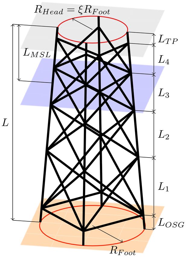
24                                                                      J. Häfele et al.: A comparison study on jacket substructures

ing problem, where the topology is fixed.1 Structural design             sign stages, where basic properties like the numbers of legs or
codes require the computation of time domain simulations                 bays are more critical than the exact dimensions of each sin-
to perform structural code checks for fatigue and ultimate               gle tube. Therefore, an optimization scheme which addresses
limit state. As environmental conditions in offshore wind                the early design phase is highly desirable to provide decision
farm locations vary strongly, commonly thousands of sim-                 guidance for experienced designers. Proposals tackling this
ulations are necessary to cover the effect of varying wind               kind of problem were given by Damiani (2016) and Häfele
and wave states for verification.2 Therefore, numerical lim-             and Rolfes (2016), where technically oriented jacket models
itations are a great issue in state-of-the-art jacket optimiza-          were proposed but lacking fatigue limit state checks in the
tion approaches. In the literature, different approaches were            first and detailed load assumptions in the second case. Based
presented to address this issue. Schafhirt et al. (2014) pro-            on the latter and with improved load assumptions, a hybrid
posed an optimization scheme based on a meta-heuristic ge-               jacket for offshore wind turbines with high rated power was
netic algorithm to guarantee global convergence. To increase             designed (Häfele et al., 2016). Due to innovative materials
the numerical efficiency, a reanalysis technique was applied.            (the technology readiness level of such a structure is still
Later, an improved approach was illustrated (Schafhirt et al.,           low), this work lacked detailed cost assumptions. Another
2016), where the load calculation was decoupled from the                 proposal for an integrated design approach was made by San-
actual tube dimensioning procedure and a simplified fatigue              dal et al. (2018), considering varying bottom widths and soil
load set (Zwick and Muskulus, 2016) was applied. Similar                 properties. This work is meant as an approach for conceptual
approaches by Chew et al. (2015, 2016) and Oest et al. (2016)            design phases. However, our conclusion on the state of the art
applied sequential quadratic or linear programming methods,              is that an optimization approach without massive limitations
respectively, with analytically derived gradients. Other op-             is still missing.
timization approaches using meta-heuristic algorithms were                  This work is intended as a contribution to the improvement
reported by AlHamaydeh et al. (2017) and Kaveh and Sa-                   of the state of the art by considering jacket optimization in
beti (2018) but without comprehensive load assumptions.                  a different way. Compared to other works in this field, the
The problem of discrete design variables was addressed by                focus is on
Stolpe and Sandal (2018). Oest et al. (2018) presented a
                                                                           1. the incorporation of topological design variables in the
jacket optimization study, where different simulation codes
                                                                              optimization problem, while the dimensioning of tubes
were deployed to perform structural code checks. All men-
                                                                              is characterized by global design variables;
tioned works, except for the last one, represent tube sizing
algorithms applied to the Offshore Code Comparison Col-                    2. more detailed cost assumptions;
laboration Continuation (OC4) jacket substructure (Popko
et al., 2014) for the National Renewable Energy Laboratory                 3. more comprehensive load sets for fatigue and ultimate
(NREL) 5 MW reference turbine (Jonkman et al., 2009),3                        limit state structural design code checks;
where the initial structural topology is maintained even in
                                                                           4. a change in the exploitation of jacket optimization re-
the case of a strong tube diameter and wall thickness varia-
                                                                              sults. This work intends to consider jacket optimization
tions. Furthermore, it can be stated that all proposals share
                                                                              as a part of the preliminary design phase because it is as-
the entire mass of the jacket as an objective function to be
                                                                              sumed that the (economically) most expensive mistakes
minimized, which is meaningful in terms of tube sizing.
                                                                              in jacket design are made at this stage of the design pro-
Due to numerical limitations, the utilized load sets are al-
                                                                              cess.
together small, for instance with low numbers of production
load cases or the omission of special extreme load events.               A basis to address these points was given by Häfele et al.
These assumptions constitute drawbacks when considering                  (2018a), where appropriate geometry, cost, and structural
jacket optimization as part of a decision process in early de-           code check models for fatigue and ultimate limit states were
                                                                         developed. In this study, these models are deployed within an
     1 This work focuses on the problem of jacket optimization and
                                                                         optimization scheme to obtain optimal design solutions for
disregards other substructure types. For a comprehensive overview        jacket substructures. A more efficient or accurate method to
of the structural optimization of wind turbine support structures,       solve the optimization problem is deliberately not provided
Muskulus and Schafhirt (2014).                                           in this study. The authors believe that there are numerous
    2 During conceptual design phases, the number of load cases is
                                                                         techniques presented in the literature that are able to solve
commonly reduced.
    3 It is worth mentioning that the Offshore Code Comparison Col-      the jacket optimization problem.
laboration Continuation (OC4) jacket is actually a structurally re-
                                                                            The paper is structured as follows. Sect. 2 describes the
duced derivation of the so-called UpWind jacket (Vemula et al.,          technical and mathematical problem statements. Both the ob-
2010), which was created to ease calculations within the verifica-       jective and the constraints are presented and explained in
tion efforts in the OC4 project. Therefore, it is not guaranteed that    Sect. 3. The optimization approach and methods to solve the
the OC4 jacket is an appropriate comparison object, as it does not       problem are discussed in Sect. 4. Section 5 illustrates the
incorporate details of tubular joints.                                   application of the approach to a test problem, a comparison

Wind Energ. Sci., 4, 23–40, 2019                                                                 www.wind-energ-sci.net/4/23/2019/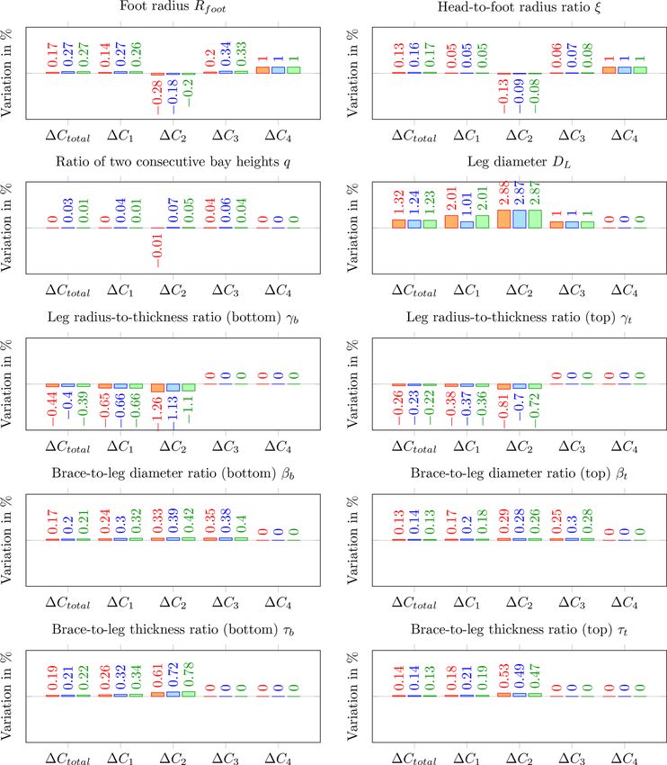
J. Häfele et al.: A comparison study on jacket substructures                                                                      25

of jackets with different topologies, performed for an NREL         In other words, a set of design variables for a parameterizable
5 MW turbine under FINO3 environmental conditions. This             structure that minimizes its costs, Ctotal , is desirable, while
section comprises a detailed setup of the problem and a dis-        fatigue and ultimate limit state constraints are satisfied; i.e.,
cussion of the results. The work ends with a consideration of       the maximal normalized tubular joint fatigue damage (among
benefits and limitations (Sect. 6) and conclusions (Sect. 7).       all tubular joints), hFLS , is less than or equal to 1,4 and the
                                                                    extreme load utilization ratio (among all tubes), hULS , is less
2    Problem statement                                              than or equal to 1.
                                                                       The total expenses are defined as an objective function
This paper presents a study on jacket substructures, based on       f (x), which depends on an array of design variables, x:
optimization. The design of jackets is a complex task that re-
                                                                    f (x) = log10 (Ctotal (x)) .                                 (1)
quires profound expertise and experience. Therefore, it has
to be clarified that this work does not provide a method re-        In this equation, the cost value is logarithmized to obviate nu-
placing established design procedures. It is rather meant as        merical issues. The constraints, h1 (x) and h2 (x), are formu-
guidance in early design phases, where it is desirable to de-       lated so as to match the requirements of mathematical prob-
fine the basic topology and dimensions of the substructure. In      lem statements; thus
industrial applications, this step is commonly highly depen-
dent on the knowledge of experienced designers. Along with          h1 (x) = hFLS (x) − 1,
this statement, it has to be pointed out that the term “optimal
                                                                    h2 (x) = hULS (x) − 1,                                       (2)
solution” may indicate a solution that it is indeed optimal
concerning the present problem formulation but not neces-           depending also on the array of design variables, x.
sarily optimal in terms of a final design due to the following        Based on the technical problem statement, we define the
aspects.                                                            mathematical problem statement in terms of a nonlinear pro-
                                                                    gram:
    – Although the approach deploys more detailed assump-
      tions on the modeling of costs and environmental con-         minf (x)
      ditions, compared to optimization approaches known
                                                                    such that x lb ≤ x ≤ x ub ,
      from the literature, it still incorporates simplifications,
      mainly for the sake of numerical efficiency.                  h1 (x) ≤ 0 and h2 (x) ≤ 0,                                   (3)

    – No sizing of each single tube is performed, for the same      where x is the array or vector of design variables, x lb and
      reason. This is a matter of subsequent design phases,         x ub are the lower and upper boundaries, respectively, f (x) is
      and tube dimensioning approaches exist in the literature.     the objective function, covering the costs related only to the
      Instead, tube dimensions are derived by global design         substructure, and h1 (x) and h2 (x) are nonlinear constraints
      variables.                                                    representing structural code checks for fatigue and ultimate
                                                                    limit state that are required to be satisfied for every design.
    – The design of pile foundation and transition piece is not
      performed in this approach. The reason is that both are       3     Objective and constraints
      considered in models of the structure and the costs but
      are not impacted by the selected design variables.            This section illustrates the jacket model, which is the basis
                                                                    for the optimization study. Moreover, the models for costs
    – Only fatigue and ultimate limit state are assumed to
                                                                    and structural design code checks are described, which depict
      be design-driving constraints. Serviceability limit state,
                                                                    the objective and constraint functions, respectively. These
      i.e., eigenfrequency constraints, is not regarded as
                                                                    models were elaborated on in a previous work (Häfele et al.,
      design-driving in this work because the modal behav-
                                                                    2018a).
      ior of a wind turbine with jacket substructure is strongly
      dominated by the relatively soft tubular tower. In addi-
      tion, a design leading to eigenfrequencies close to 1P        3.1    Jacket modeling and design variables
      or 3P excitation would probably fail due to high fa-          In this work, it is assumed that a jacket substructure can be
      tigue damage. Although the modal behavior is also im-         described by 20 parameters in total, of which 10 define topol-
      pacted by the foundation, this is not significant here, as    ogy, 7 tube dimensions, and 3 material properties. Topologi-
      no foundation design is performed.                            cal parameters are the number of legs, NL , number of bays,
                                                                    NX (both integer variables), foot radius, Rfoot , head-to-foot
   The overall goal of jacket optimization can be interpreted
                                                                    radius ratio, ξ , jacket length, L, elevation of the transition
as a cost minimization problem involving certain design con-
straints. As stated before, it is assumed that the design-            4 All fatigue damage is normalized so that the lifetime fatigue
driving constraints of jackets are fatigue and extreme loads.       damage corresponds to a value of 1.

www.wind-energ-sci.net/4/23/2019/                                                                  Wind Energ. Sci., 4, 23–40, 2019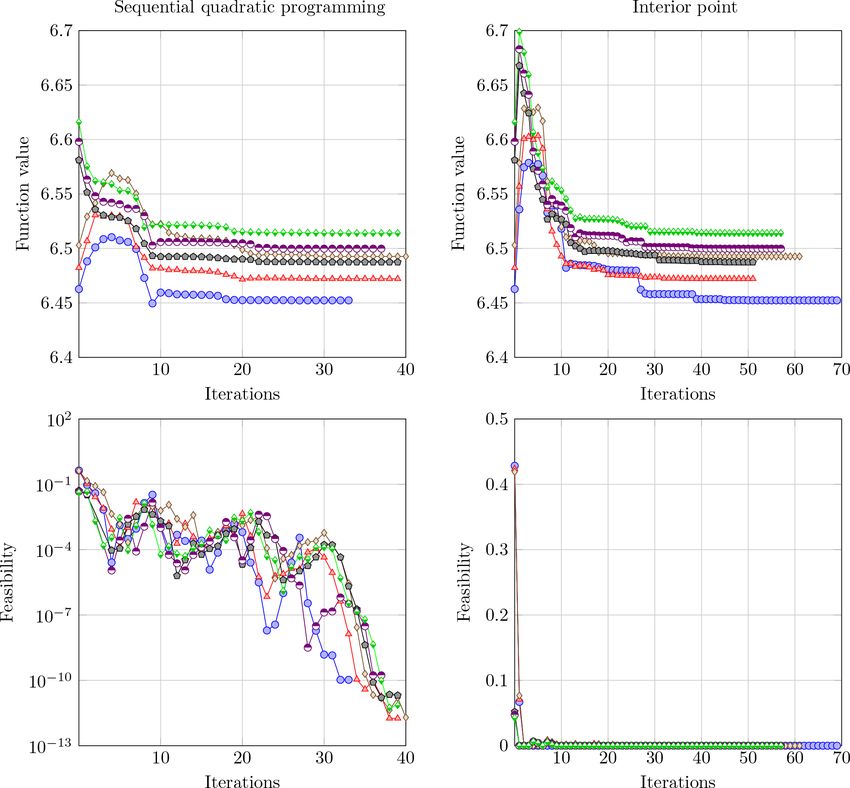
26                                                                      J. Häfele et al.: A comparison study on jacket substructures

                                                                         mension of 12:

                                                                         x = (NL NX Rfoot ξ q DL γb γt βb βt τb τt )T .                (4)

                                                                         The number of design variables is not necessarily minimal,
                                                                         but, on the one hand, mathematically manageable and, on the
                                                                         other hand, meaningful from the technical point of view.

                                                                         3.2   Cost function (objective)

                                                                         The total capital expenses, Ctotal , comprise several terms, Cj ,
                                                                         expressed as the sum of so-called factors, cj , weighted by
                                                                         unit costs, aj :5
                                                                                        X              X
                                                                         Ctotal (x) =       Cj (x) =         aj cj (x).                (5)

                                                                         A factor may be any property of the structure describing a
                                                                         cost contribution that can be expressed in terms of the design
                                                                         variables. A pure mass-dependent cost modeling approach,
Figure 1. Jacket geometry model with variables characterizing the        as used in most optimization approaches, would involve only
topology of the structure, shown exemplarily for a jacket with four      one factor, while no unit cost value is required for weighting.
legs, four bays, and mud braces. The ground layer is illustrated by
                                                                         However, a realistic cost assessment involves more than only
the orange surface and the mean sea level and transition piece layers
by the blue and gray surfaces, respectively.
                                                                         the structural mass. For example, in the case of a structure
                                                                         with very lightweight tubes but many bays, it can be imag-
                                                                         ined that the manufacturing costs tend to be a cost-driving
                                                                         factor. To consider known, important impacts on jacket cap-
                                                                         ital expenses, seven factors are incorporated, namely the fol-
piece over mean sea level, LMSL , lowermost segment height,              lowing:
LOSG , uppermost segment height, LTP , the ratio of two con-
secutive bay heights, q, and a boolean flag, xMB , determining              – expenses for material, C1 , depending on the mass, c1 :
whether the jacket has mud braces (horizontal tubes below
the lowermost layer of K joints) or not. The topology of one                                           NX
                                                                                                                              !
example with four legs (NL = 4), four bays (NX = 4), and
                                                                                                       X         βi τi   τ2
                                                                               c1 (x) =2ρNL π DL2                      + i2
mud braces xMB = true is shown in Fig. 1. The tube sizing                                              i=1
                                                                                                                 2γi    4γi
parameters are the leg diameter, DL , and six dependent pa-                             s                                   !
rameters defining relations between tube diameters and wall                                    L2i                        2 ϑ 2
                                                                                                   + (Ri + Ri+1 ) sin
thicknesses at the bottom and top of the structure: γb and                                cos2 8p                           2
γt are the leg radius to thickness ratios, βb and βt are the                                                             !
                                                                                                                     τb2

brace-to-leg diameter ratios, and τb and τt are the brace-to-                                          2 βb τ b                       ϑ
                                                                                        + xMB ρNL π DL           + 2 2R1 sin
leg thickness ratios, where the indices b and t indicate values                                            2γb      4γb               2
at the bottom and the top of the jacket, respectively. Using                                        N X
                                                                                                                         !
                                                                                                    X        1        1      Lm,i
dependent parameters is beneficial because structural code                              + ρNL π DL2              + 2
checks are valid for certain ranges of these dependent vari-                                        i=1
                                                                                                            2γ i    4γ i
                                                                                                                           cos  (8s )
                                                                                                           !               !
ables. Furthermore, for structural analysis, the material is as-                              1         1       Li − Lm,i
sumed to be isotropic and can thus be described by a Young’s                            +         + 2
                                                                                            2γi+1 4γi+1          cos (8s )
modulus, E, a shear modulus, G, and density, ρ.                                                                    !
   To decrease the dimension of the problem, height mea-                                          2     1      1       LOSG
sures related to the location of the wind farm (L, LMSL ,                               + ρNL π DL        +
                                                                                                      2γb 4γb2 cos (8s )
LOSG , LTP ) and the material parameters (E, G, ρ) are fixed.
In addition, it is supposed that each design has mud braces                                            1       1        LTP
                                                                                        + ρNL π DL2       + 2                 ;         (6)
(xMB = true). Although designs without mud braces are also                                            2γt 4γt cos (8s )
imaginable, fixing this parameter is advantageous, as it is not
continuous. The array of design variables therefore has a di-               5 Unit cost values are given in Sect. 5.3.

Wind Energ. Sci., 4, 23–40, 2019                                                                     www.wind-energ-sci.net/4/23/2019/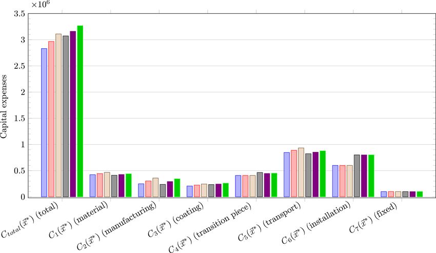
J. Häfele et al.: A comparison study on jacket substructures 27
– expenses for fabrication, C2 , depending on the entire In these equations, ϑ is the angle enclosed by two jacket legs:
volume of welds, c2 :
2π
NX
! ϑ= . (13)
X DL2 τi2 t0 DL τi NL
c2 (x) =2NL π DL βi + √
i=1 8γi2 2 2γi Bay heights, Li , intermediate bay heights, Lm,i , radii, Ri ,
s s and intermediate radii, Rm,i , are calculated by the following
1 1 1 1
+ + + equations:
2 2 2 2
2sin ψ1,i 2sin ψ2,i
s !! L − LOSG − LTP
1 1 Li = PNX n−i , (14)
+ + n=1 q
2sin2 ψ3,i 2
L i Ri
! Lm,i = , (15)
DL2 τb2 t0 DL τb Ri + Ri+1
+ 2xMB NL π DL βb + √
8γb2
!
2 2γb i−1
X
Ri = Rfoot − tan (8s ) LOSG + Ln , (16)
2 1 1
NX DL min γ 2 , γ 2
X
n=1
i i+1
!
+ NL π DL i−1
X
i=1
8 Rm,i = Rfoot − tan (8s ) LOSG + Ln + Lm,i , (17)
n=1
DL t0 min γ1i , γi+1
1
with the spatial batter angle, 8s :
+ √ ; (7)
2 2
Rfoot (1 − ξ )
8s = arctan . (18)
L
– coating costs, C3 , depending on the outer surface area
The interconnecting tube angles, ψ1,i , ψ2,i , and ψ3,i , are
of all tubes, c3 :
!
Rfoot (1 − ξ ) sin ϑ2 cos 8p
NX π
c3 (x) =2NL π DL
X ψ1,i = − arctan
2 L
i=1 !
s ! Lm,i
L2i 2 2 ϑ − arctan , (19)
Ri sin ϑ2 cos 8p
βi + (Ri + Ri+1 ) sin
cos2 8p 2 !
Rfoot (1 − ξ ) sin ϑ2 cos 8p
ϑ π
+ xMB NL π DL βb 2R1 sin ψ2,i = + arctan
2 2 L
!
L Lm,i
+ NL π DL ; (8) − arctan , (20)
cos (8s ) Ri sin ϑ2 cos 8p
– costs for the transition piece, C4 , proportional to the
!
product of head radius and number of jacket legs, c4 : Lm,i
ψ3,i = 2 arctan , (21)
Ri sin ϑ2 cos 8p
c4 (x) = NL Rfoot ξ ; (9)
with the planar batter angle, 8p :
– expenses for transport, C5 , expressed by the mass-
dependent factor, c5 : Rfoot (1 − ξ ) sin ϑ
!
2
8p = arctan . (22)
c5 (x) = c1 (x); (10) L
– and installation costs, C6 , modeled by a factor only de- γi , βi , and τi represent the ratios of leg radius-to-thickness,
pending on the number of jacket legs, c6 : brace-to-leg diameter, and brace-to-leg thickness of the ith
bay, respectively, obtained by linear stepwise interpolation
c6 (x) = NL . (11) and counted upwards.
The cost modeling is based on several simplifications and
Fixed expenses, C7 , are not dependent on any jacket param- assumptions. The mass-proportional modeling of material
eter at all. Therefore, the factor, c7 , simply takes costs, C1 , is straightforward. Fabrication costs, C2 , mainly
arise from welding and grinding processes. Although the ac-
c7 (x) = 1. (12) tual manufacturing processes are quite complex, the entire
www.wind-energ-sci.net/4/23/2019/ Wind Energ. Sci., 4, 23–40, 201928 J. Häfele et al.: A comparison study on jacket substructures
volume of welds can be regarded as a measure of the ac- To face this issue, a surrogate modeling approach based
tual costs. Coating costs, C3 , are quite easy to determine on Gaussian process regression (GPR) is deployed. It was
by the outer surface area of all tubes, i.e., the area to be shown previously (Häfele et al., 2018a) that good regression
coated. There may be synergy effects when coating larger results can be obtained by GPR for this purpose. In addi-
areas, but these are neglected. The expenses for the (stellar- tion, the regression process relies on a mathematical process
type) transition piece, C4 , are assumed to be proportional to that can be interpreted easily and adapted to prior knowledge
the head radius and the number of legs. There are more de- of the underlying physics. In the present case, the procedure
tailed approaches for this purpose, but no design of the tran- is as follows: a load set with a defined number of design
sition piece is performed, which requires a simple approach. load cases is the basis for structural code checks. The size
The determination of transport costs, C5 , is very difficult. In of the load sets and parameters of environmental and oper-
this work, a mass-dependent approach was selected, which ational conditions are predetermined so as to represent the
is, however, a large simplification. The mass dependence re- loads on the turbine adequately. With these load sets, numer-
flects that barges have a limited transport capacity, which is ical simulations are performed with the aero–hydro–servo–
at least to some extent mass-dependent or dependent on fac- elastic simulation code FAST to obtain output data for the
tors partially related to mass (like the space on the deck of input space of the surrogate model.6 As this procedure re-
the barge covered by the jacket). Installation costs, C6 , cover quires much computational effort, the input space is limited
both the material and the manufacturing of the foundation to 200 jacket samples (excluding validation samples) in each
and the installation at the wind farm location. In the case of a case as a basis for both surrogate models (fatigue and ulti-
pile foundation, these costs are mainly governed by the num- mate limit state),7 obtained by a Latin hypercube sampling
ber of piles, which is equal to the number of legs. The fixed of the input space. In both cases, the results are vectors of
expenses, C7 , are not vital for the solution of the optimiza- output variables, where each element corresponds to a row
tion problem but are required to shift the costs to more realis- in the matrix of inputs, comprising parameters of the input
tic values by covering expenses for cranes, scaffolds, and so space. Both (input matrix and output vector) build the train-
forth. ing data. For each new sample, the corresponding output (re-
sult of a structural code check) is evaluated by GPR.8 The
3.3 Structural code checks (constraints)
specific surrogate models for the considered test problems
were derived in a previous work (Häfele et al., 2018a), which
To check jacket designs – i.e., sets of design variables – revealed that a Matérn 5/2 kernel function is well-suited for
for validity concerning fatigue and extreme load resistance, the present application.
structural design code checks are performed. The standards
DNV GL RP-C203 (DNV GL AS, 2016) for fatigue and 3.3.1 Fatigue limit state
NORSOK N-004 (NORSOK, 2004) for ultimate limit state
checks are adopted. Both are widely accepted for practical The evaluation of fatigue limit state code checks requires
applications and were used to design the UpWind (Vemula many simulations considering design load cases (DLCs) 1.2
et al., 2010) and INNWIND.EU (von Borstel, 2013) refer- and 6.4 production load cases according to IEC 61400-3 (In-
ence jackets. ternational Electrotechnical Commision, 2009). Under de-
Commonly, the numerical demand of structural code fined conditions (5 MW turbine, 50 m water depth, FINO3
checks is one of the main problems in jacket optimization. To environmental conditions), the required number of design
cover the characteristics of environmental impacts on wind load cases with respect to uncertainty was analyzed in pre-
turbines, representative loads are to be used for the load as- vious papers (Häfele et al., 2017, 2018b). In these papers, a
sessment. This involves numerous load simulations to con- load set with 2048 design load cases was gradually reduced
sider all load combinations that might occur, particularly in to smaller load sets. A reduced load set with 128 design load
the fatigue case, where the excitation is extrapolated for the cases turned out to be a good compromise between accuracy,
entire turbine lifetime. As not only the number of load simu- as the uncertainty arising from the load set reduction is ac-
lations but also the duration (in the case of time domain sim- ceptable in this case, and numerical effort, which is signifi-
ulations) correlates to a high demand in numerical capacity, cantly smaller compared to the initial load set; i.e., consid-
most approaches deploy very simple load assumptions like ering two X-joint positions, the standard deviation of fatigue
one design load case per iteration, as already discussed. Al- 6 FASTv8 (National Wind Technology Center Information Por-
together, a high numerical effort is required. Utilizing simpli- tal, 2016) was used for this study.
fied load assumptions like equivalent static loads, where the 7 All parameters of these jacket samples are given in the publica-
substructure decoupled from the overlying structure and all tion where the surrogate modeling approach was reported (Häfele
interactions are neglected, depicts, however, a massive sim- et al., 2018a).
plification in the case of a wide range of design variables. By 8 For the background theory of GPR, the reader is referred to
contrast, a pure simulation-based optimization is not appli- Rasmussen and Williams (2008), which is the standard reference in
cable due to the aforementioned reasons. this field.
Wind Energ. Sci., 4, 23–40, 2019 www.wind-energ-sci.net/4/23/2019/J. Häfele et al.: A comparison study on jacket substructures 29
damage increases by a factor of approximately 4 in the case 4 Optimization approach and solution methods
of a 16-fold load set reduction (from 2048 to 128 design load
cases). The actual fatigue assessment involves time domain The optimization problem incorporates a mixed-integer for-
simulations, an application of stress concentration factors ac- mulation (due to discrete numbers of legs and bays of the
cording to Efthymiou (1988) to consider the amplification of jacket). In order to address this issue, the mixed-integer prob-
stresses due to the geometry of tubular joints, rain flow cycle lem is transferred to multiple continuous problems by solv-
counting, and a lifetime prediction by S-N curves and linear ing solutions with a fixed number of legs and bays. As only
damage accumulation.9 The output value hFLS is the most a few combinations of these discrete variables are regarded
critical fatigue damage among all damage values of the entire as realistic solutions for practical applications, this proce-
jacket (evaluated in eight circumferential points around each dure leads to a very limited number of subproblems but eases
weld), normalized by the calculated damage at design life- the mathematical optimization process significantly. Further-
time. A design lifetime of 30 years is assumed, from which more, the optimization problem is generally non-convex; i.e.,
25 years are the actual lifetime of the turbine and 5 years are a local minimum in the feasible region satisfying the con-
added to consider malicious fatigue damage during the trans- straints is not necessarily a global solution. This is addressed
port and installation process. Moreover, a partial safety factor by repeating the optimization with multiple starting points.
of 1.25 is considered in the fatigue assessment. The development of new or improved optimization meth-
ods to solve the numerical optimization problem is not in the
scope of this work because there are methods presented in
3.3.2 Ultimate limit state the literature that are known to be suitable for this purpose.
Meta-heuristic algorithms like genetic algorithms or particle
The standard IEC 61400-3 (International Electrotechnical swarm optimization are not considered in this work because
Commision, 2009) requires several design load cases to per- they are known to be slow. With regard to efficiency and
form structural code checks for the ultimate limit state. How- accuracy, two methods are regarded as the most powerful
ever, not every design load case is critical for the design of for optimization involving nonlinear constraints: sequential
a jacket substructure. The relevant ones were analyzed and quadratic programming (SQP) and interior-point (IP) meth-
found to be DLC 1.3 (extreme turbulence during production), ods (Nocedal and Wright, 2006). SQP methods are known
1.6 (extreme sea state during production), 2.3 (grid loss fault to be efficient, when the numbers of constraints and design
during production), 6.1 (extreme sea state during idle), and variables are of the same order of magnitude. An advantage
6.2 (extreme yaw error during idle) for a turbine with a rated is that these methods usually converge better when the prob-
power of 5 MW, under FINO3 environmental conditions and lem is badly scaled. In theory, IP methods have better con-
a water depth of 50 m. Extreme load parameters are derived vergence properties and often outperform SQP methods on
by the block maximum method (see Agarwal and Manuel, large-scale or sparse problems. In this work, both approaches
2010), where the environmental data are divided into many are used to solve the jacket optimization problem.10 They are
segments featuring similarly distributed data. From this data outlined briefly in the following.
set, the maximum values are extracted. Based on these max-
ima, return values (as required by IEC 61400-3) of environ-
mental states are computed. To conduct the structural code 4.1 Sequential quadratic programming method
checks for the ultimate limit state, time domain simulations
are performed and evaluated with respect to the extreme load In principle, SQP can be seen as an adaption of New-
of the member, where the highest utilization ratio occurs. The ton’s method to nonlinear constrained optimization prob-
result hULS is a value that approaches 0 in the case of infi- lems, computing the solution of the Karush–Kuhn–Tucker
nite extreme load resistance and 1 in the case of equal re- equations (necessary conditions for constrained problems).
sistance and loads, implying that values greater than 1 are Here, a common approach is deployed, based on the works of
related to designs not fulfilling the ultimate limit state code Biggs (1975), Han (1977), and Powell (1978a, b). In the first
check. The procedure considers combined loads with axial step, the Hessian of the so-called Lagrangian (a term incorpo-
tension, axial compression, and bending, with and without rating the objective and the sum of all constraints weighted
hydrostatic pressure, which may lead to failure modes like by Lagrange multipliers) is approximated by the Broyden–
material yielding, overall column buckling, local buckling, Fletcher–Goldfarb–Shanno method (Fletcher, 1987). In the
or any combination of these. A global buckling check is not next step, a quadratic programming subproblem is built,
performed in this study, as it is known to be uncritical for where the Lagrangian is approximated by a quadratic term
jacket substructures (Oest et al., 2016). and linearized constraints. This subproblem can be solved by
any method able to solve quadratic programs. An active-set
9 It has to be stated that there are several ways to determine stress
concentration factors for tubular joints. This is the approach pro- 10 The function fmincon in MATLAB R2017b was used for this
posed by the standard DNV GL RP-C203 (DNV GL AS, 2016). study.
www.wind-energ-sci.net/4/23/2019/ Wind Energ. Sci., 4, 23–40, 201930 J. Häfele et al.: A comparison study on jacket substructures
method described by Gill et al. (1981) is deployed for this abilistic loads (Hübler et al., 2017). The probabilistic load
task. The procedure is repeated until convergence is reached. set, which is based on probability density functions of en-
vironmental state parameters and reduced in size compared
4.2 Interior-point method to full load sets used by industrial wind turbine designers,
was described in recent studies (Häfele et al., 2017, 2018b).
IP methods are barrier methods; i.e., the objective is approx- However, there are two drawbacks that have to be mentioned
imated by a term that incorporates a barrier term, expressed when using this data. First, the FINO3 platform was built at a
by a sum of logarithmized slack variables. The actual prob- location with quite a shallow water depth of 22 m, though the
lem itself, just like in SQP, is solved as a sequence of sub- jacket is supposed to be an adequate substructure for water
problems. In this work, an approach is deployed, which may depths above 40 m and the design water depth in this study is
switch between line search and trust region methods to ap- 50 m. Nevertheless, this procedure was also performed in the
proximated problem, depending of the success of each step. UpWind project for the design of the OC4 jacket, where the
If the line search step fails, i.e., when the projected Hessian K13 deep-water site was considered. Second, the soil proper-
is not definitively positive, the algorithm performs a trusted ties of the Offshore Code Comparison Collaboration (OC3)
region step, where the method of conjugate gradients is de- (Jonkman and Musial, 2010) are adopted to compute founda-
ployed. The algorithm is described in detail by Waltz et al. tion inertias and stiffnesses, as these values are unknown for
(2006). the FINO3 location. Moreover, it is assumed that the struc-
tural behavior of the OC4 jacket pile foundation is valid for
5 Jacket comparison study all jacket designs, even with varying leg diameters and thick-
nesses.
In this section, the proposed approach is applied to find and
compare optimal jacket designs for the NREL 5 MW refer- 5.3 Boundaries of design variables and other
ence turbine (Jonkman et al., 2009). The environmental con- parameters
ditions are adopted from measurements recorded at the re-
search platform FINO3 in the German North Sea. The boundaries are chosen conservatively by means of quite
narrow design variable ranges (see Table 1), i.e., meaning-
ful parameters that do not exhaust the possible range given
5.1 Reference turbine
by the structural code checks, in a realistic range around the
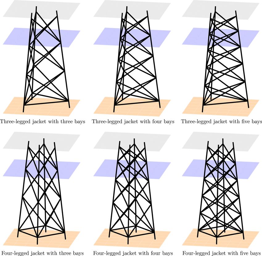
The NREL 5 MW reference turbine, which was published al- values of the OC4 jacket (Popko et al., 2014). Only three- or
most 1 decade ago as a proposal to establish a standardized four-legged structures with three, four, and five bays are re-
turbine for scientific purposes, is still an object of many stud- garded as valid solutions for this study. The fixed design vari-
ies in the literature dealing with intermediate- to high-power ables are, if possible, adopted from the OC4 jacket, which
offshore wind applications. In fact, the market already pro- can be seen as a kind of reference structure in this case. The
vides turbines with 8 MW and aims for even higher ratings. material is steel (S355), with a Young’s modulus of 210 GPa,
Choosing this reference turbine is motivated by its excellent a shear modulus of 81 GPa, and a density of 7850 kg m−3 .
documentation and accessibility. According to DNV GL AS (2016), an S-N curve with an en-
The rotor has a hub height of 90 m, and the rated wind durance stress limit of 52.63×10⁶ N m−2 at ×107 cycles and
speed is 11.4 m s−1 , where the rotor speed is 12.1 min−1 . slopes of 3 and 5 before and after endurance limit (curve T ),
This is equal to 1P and 3P excitations of 0.2 and 0.6 Hz, re- respectively, is applied. The cost model parameters or unit
spectively. The critical first fore–aft and side–side bending costs, respectively, are adopted from the mean values given
eigenfrequencies of the entire structure are about 0.35 Hz and in Häfele et al. (2018a) and set to a1 = 1.0 kg−1 (material),
do not differ very much when considering only reasonable a2 = 4.0 × 10⁶ m−3 (fabrication), a3 = 1.0 × 10² m−2 (coat-
structural designs for the jacket because the modal behavior ing), a4 = 2.0 × 10⁴ m−1 (transition piece), a5 = 2.0 kg−1
is strongly driven by the relatively soft tubular tower. (transport), a6 = 2.0 × 10⁵ (installation), and a7 = 1.0 × 10⁵
(fixed). With these values, the cost function returns a dimen-
sionless value, also interpretable as capital expenses in EUR.
5.2 Environmental conditions and design load sets
Due to excellent availability, the environmental data are de- 5.4 Results and discussion
rived from measurements taken from the offshore research
platform FINO3, located in the German North Sea close to To resolve the mixed-integer formulation of the optimization
the wind farm “alpha ventus”. Compared to the environmen- problem into continuous problems, six subproblems with
tal conditions documented in the UpWind design basis (Fis- three legs and three bays (NL = 3, NX = 3), three legs and
cher et al., 2010), the FINO3 measurements are much more four bays (NL = 3, NX = 4), three legs and five bays (NL =
comprehensive and allow for a better estimation of probabil- 3, NX = 5), four legs and three bays (NL = 4, NX = 3), four
ity density functions as inputs for the determination of prob- legs and four bays (NL = 4, NX = 4), and four legs and
Wind Energ. Sci., 4, 23–40, 2019 www.wind-energ-sci.net/4/23/2019/J. Häfele et al.: A comparison study on jacket substructures 31
Table 1. Boundaries of jacket model parameters for design of experiments. Topological, tube sizing, and material parameters are separated
into groups; single values mean that the corresponding value is held constant.
Parameter Description Lower boundary Upper boundary
NL Number of legs 3 4
NX Number of bays 3 5
Rfoot Foot radius 6.792 m 12.735 m
ξ Head-to-foot radius ratio 0.533 0.733
L Entire jacket length 70.0 m
LMSL Transition piece elevation over mean sea level 20.0 m
LOSG Lowest leg segment height 5.0 m
LTP Transition piece segment height 4.0 m
q Ratio of two consecutive bay heights 0.640 1.200
xMB Mud brace flag true (1)
DL Leg diameter 0.960 m 1.440 m
γb Leg radius-to-thickness ratio (bottom) 12.0 18.0
γt Leg radius-to-thickness ratio (top) 12.0 18.0
βb Brace-to-leg diameter ratio (bottom) 0.533 0.800
βt Brace-to-leg diameter ratio (top) 0.533 0.800
τb Brace-to-leg thickness ratio (bottom) 0.350 0.650
τt Brace-to-leg thickness ratio (top) 0.350 0.650
E Material Young’s modulus 2.100 × 10¹¹ N m−2
G Material shear modulus 8.077 × 10¹⁰ N m−2
ρ Material density 7.850 × 10³ kg m−3
five bays (NL = 4, NX = 5) were solved using the SQP and has a leg diameter, DL , of 1.2 m, and entirely constant tube
IP methods. Therefore, multiple solutions are discussed and dimensions from bottom to top, i.e., leg radius-to-thickness
compared in the following. The optimization problem is non- ratios, γb and γt , of 15, brace-to-leg diameter ratios, βb and
convex; i.e., a local minimum in the feasible region satisfying βt , of 0.5, and brace-to-leg diameter ratios, τb and τt , of 0.5.
the constraints is not necessarily a global solution. In the- The optimization process needed between 30 and 40 itera-
ory, both algorithms converge from remote starting points. tions using the SQP method and between 50 and 70 itera-
However, to guarantee global convergence to some extent, tions using the IP method to converge. It is worth mention-
all six combinations of fixed-integer variables were solved ing that the maximum constraint violation (feasibility) of the
using 100 randomly chosen starting points. Installation costs three-legged designs was higher at the beginning of the opti-
and fixed expenses were excluded from the objective func- mization process but converges stably. For the same reason,
tion and included again after the optimization procedure be- the four-legged designs have a higher improvement poten-
cause these terms do not have an effect on the individual tial compared to the initial solution. The accuracy obtained
optimization problems.11 Gradients were computed by fi- by both methods is similar. The solutions are all feasible be-
nite differences. The optimization terminated, when the first- cause they fulfill the Karush–Kuhn–Tucker conditions, and
order optimality and feasibility measures were both less than all constraint violations are around zero. Therefore, the op-
1 × 10⁻⁶ . There was no limit to the maximum number of it- tima are probably global optima for the given design variable
erations. boundaries.
The optimal solutions of all six subproblems do not de- The optimal solutions obtained by the sequential quadratic
pend on the starting point when using both optimization programming method are illustrated in Table 2.12 Addition-
methods because there is only one array of optimal design ally, the topologies of all optimal solutions are shown in
variables in each case. The convergence behavior of both op- Fig. 3. With respect to the constraints and assumptions of this
timization methods is illustrated in Fig. 2, where the OC4 study (5 MW turbine, 50 m water depth, given environmen-
jacket with varying numbers of legs and bays was assumed tal conditions and cost parameters), jackets with three legs
as the starting point. This structure has a foot radius, Rfoot , are beneficial in terms of capital expenses. The three-legged
of 8.79 m, a head-to-foot radius ratio, ξ , of 0.67, and a ra- jacket with three bays (NL = 3, NX = 3) is the best solu-
tio of two consecutive bay heights, q, of 0.8. Moreover, it tion, i.e., is related to the lowest total expenditures, among
11 The values shown in the following include all cost terms. The 12 As the accuracy of the SQP and IP methods is similar here, only
exclusion is only performed during optimization. results obtained by the SQP method are shown in the following.
www.wind-energ-sci.net/4/23/2019/ Wind Energ. Sci., 4, 23–40, 201932 J. Häfele et al.: A comparison study on jacket substructures
Figure 2. Function and feasibility (maximum constraint violation) values during the optimization procedure of all six subproblems (blue line
with circles: jacket with three legs and three bays; red line with triangles: jacket with three legs and four bays; brown line with diamonds:
jacket with three legs and five bays; black line with pentagons: jacket with four legs and three bays; violet line with half-filled circles: jacket
with four legs and four bays; green line with half-filled diamonds: jacket with four legs and five bays). The starting point (iteration “0”) is
the OC4 jacket with a varying number of legs and bays in all cases. One iteration involves 11 evaluations of the objective function and the
nonlinear constraints.
Table 2. Optimal solutions of design variables x ∗ obtained by the sequential quadratic programming method for fixed values of NL and NX .
Optimal solution
NL 3 3 3 4 4 4
NX 3 4 5 3 4 5
Rfoot in m 12.735 12.735 12.735 10.894 10.459 10.549
ξ 0.533 0.533 0.533 0.533 0.533 0.533
q 0.937 0.941 0.936 0.813 0.809 0.977
DL in m 1.021 1.021 1.023 0.960 0.960 0.960
x∗
βb 0.800 0.800 0.800 0.800 0.799 0.787
βt 0.800 0.800 0.800 0.800 0.800 0.800
γb 12.000 12.000 12.000 12.680 12.259 12.000
γt 16.165 16.029 15.928 18.000 18.000 18.000
τb 0.513 0.505 0.493 0.497 0.493 0.478
τt 0.472 0.466 0.454 0.383 0.387 0.383
Overall mass in t 423 444 467 412 426 439
f (x ∗ ) = log10 Ctotal (x ∗ )
6.452 6.472 6.493 6.487 6.500 6.514
h1 (x ∗ ) = hFLS (x ∗ ) − 1 1.172 × 10⁻¹⁰ 3.966 × 10⁻¹¹ 1.151 × 10⁻¹⁰ 1.450 × 10⁻¹⁰ −1.056 × 10⁻¹⁰ −1.721 × 10⁻¹⁰
h2 (x ∗ ) = hULS (x ∗ ) − 1 7.819 × 10⁻¹⁰ 2.678 × 10⁻¹⁰ 1.093 × 10⁻¹⁰ 3.978 × 10⁻¹⁰ 3.980 × 10⁻¹⁰ 5.995 × 10⁻¹⁰
Wind Energ. Sci., 4, 23–40, 2019 www.wind-energ-sci.net/4/23/2019/J. Häfele et al.: A comparison study on jacket substructures 33 Figure 3. Topologies of optimal solutions x ∗ . All images are displayed at the same scale. Line widths are not correlated to tube dimensions. the considered jackets. The solutions show some interesting at the jacket bottom, the values of γt are much higher. The specialties. The foot radii, Rfoot , are at the upper boundaries impact of all design variables on the objective function is eas- in the case of the three-legged structures, while the head-to- ier to understand when the sensitivities of cost model terms foot radius ratios, ξ , are at the lower boundaries. Probably to variations in design variables are considered. In Fig. 4, this arises from the combination of cost function and non- each subplot shows the variation in the total costs, Ctotal , and linear constraints, where a large foot radius is quite bene- the cost function terms C1 (proportional to C5 ), C2 , C3 , and ficial because it generally provides a higher load capacity, C4 due to a 1 % one-at-a-time variation in each continuous while a small head radius is favorable due to lower transi- design variable in three different phases of the optimization tion piece costs. In the four-legged case, the foot radii are process (initial, intermediate, and final phase). The terms C6 lower but still relatively high. In any case, it seems to be and C7 are not impacted by any continuous design variable beneficial, when the ratio of two consecutive bay heights, q, and therefore not considered. For instance, a 1 % increase is slightly below 1 (lower bays are higher than upper bays). in the foot radius, Rfoot , causes increasing material costs of Concerning tube dimensions, the leg diameters, DL , are rela- 1C1 = 0.14 %, evaluated for the initial design, but increas- tively small, in the case of the four-legged jackets even at the ing material costs of 1C1 = 0.26 %, evaluated for the opti- lower boundary. The structural load capacity is established mal design. Therefore, the sensitivity of this cost term varies by high brace diameters (represented by design variables βb during the optimization process. In contrast, the variation in and βt , values at the bottom and top of the structures both transition piece expenses does not change (which is reason- at upper boundaries). The brace thicknesses, represented by able because this term only depends linearly on the number τb and τt , show intermediate values in the range of design of legs, NL , the foot radius, Rfoot , and the head-to-foot ra- variables, while the values for τt are higher in the case of dius ratio, ξ ). In general, Fig. 4 shows that there is no design three-legged designs. Moreover, the structural resistance is variable with a strongly varying impact on any term of the strongly driven by the leg thicknesses. While the optimal val- cost function. It can also be concluded that tube sizing vari- ues of γb are low in each case, implying high leg thicknesses ables impact the costs much more strongly than topological www.wind-energ-sci.net/4/23/2019/ Wind Energ. Sci., 4, 23–40, 2019
34                                                                    J. Häfele et al.: A comparison study on jacket substructures

variables, disregarding the number of legs and bays. Among             times of about 15 to 30 min on a single core of a work sta-
the considered design variables, the leg diameter, DL , and            tion with an Intel Xeon E5-2687W v3 central processing unit
leg radius-to-thickness ratios, γb and γt , are design-driving         and 64 GB random access memory. Compared to simulation-
(together with the number of legs, NL ) due to a significant           based approaches, this can be regarded as very fast. The num-
impact both on the costs and on the structural code checks.            ber of iterations may be decreased, when using analytical
In addition, an interesting specialty is featured by the cost          gradients of the objective function because using finite dif-
term C4 , which is only impacted by topological design vari-           ferences is generally more prone to numerical errors but is
ables, more precisely the foot radius, Rfoot , and the head-to-        not vital at this level of computational expenses. It has to be
foot radius ratio, ξ . As a large foot radius, Rfoot , is needed to    pointed out that the training data set of the surrogate mod-
establish structural resistance, this cost term penalizes large        els required 200 × 128 = 25 600 time domain simulations in
head-to-foot radius ratios, ξ . For this reason, this value is at      the fatigue and 200 × 10 = 2000 in the ultimate limit state
the lower boundary for all design solutions.                           case, thus 27 600 simulations in total, excluding validation
   Regarding the costs of the jackets, the best solution with          samples. However, for the computation of the training data,
three legs and three bays is related to capital expenses of            a compute cluster was utilized, which allows for the com-
106.452 = 2 831 000. Altogether, this is a meaningful value            putation of many design load cases in parallel. Therefore,
and the designs are not far off from structural designs that           the presented approach based on GPR allows for outsourcing
are known from practical applications because it has al-               computationally expensive simulations on high-performance
ready been reported in the literature that three-legged de-            clusters, while the closed-loop optimization, which cannot
signs may be favorable in terms of costs (Chew et al., 2014)           be parallelized completely, can be run on a workstation with
and three-legged structures have already been built. How-              lower computational capacity.
ever, the other solutions are more expensive but not com-                 The question remains what happens when some cost terms
pletely off. As there is some uncertainty in the unit costs, the       are neglected. An associated question is how the approach
other jackets may also be reasonable designs with slightly             performs compared to a pure mass-dependent one, which
different boundaries. A more detailed cost breakdown is                can be regarded as state of the art in jacket optimization.
given in Fig. 5, which shows the cost contributions of all             For this purpose, all unit costs except a1 were set to zero
six structures and where the actual cost savings come from.            and the optimization procedure was repeated using the se-
The lightest structure is the four-legged jacket with three            quential quadratic programming method. The results, includ-
bays, while the three-legged jacket with five bays is the              ing optimal design variables and resulting values of objective
heaviest one, which is illustrated by the expenses for mate-           and constraint functions, are shown in Table 3. Under these
rial and transport according to the cost model used for this           assumptions, the four-legged jackets are better (in terms of
study. Nevertheless, the mass of all structures is quite sim-          minimal mass) than the three-legged ones. Interestingly, sim-
ilar. Other than expected, the jacket with the lowest expen-           ilar design variables are obtained when comparing these val-
ditures for manufacturing is also the four-legged one with             ues to the ones obtained by the more comprehensive cost
three bays and not the three-legged jacket with three bays,            model in Table 2, particularly in the case of the three-legged
which has the least number of joints. The three-legged struc-          jackets. The resulting objective function values are, in com-
tures benefit – from the economic point of view – mainly               parison, similar to the material costs in Fig. 5. In other words,
from lower expenses for coating, the transition piece, and,            a pure mass-dependent cost function approach yields approx-
most distinctly, installation costs. In total, these contribu-         imately proportional costs, when the installation costs (de-
tions add up to lower costs of the three-legged jackets, ex-           pending on the number of legs) are considered, and similar
cept for the one with five bays (106.493 = 3 112 000), which           designs. The reason for this is that all cost terms C1 . . .C5
is more expensive than the four-legged one with three bays             depend in some way on the tube dimensions and the topol-
(106.487 = 3 069 000). The most expensive jackets are the              ogy does not impact the costs to a great extent, as seen in
four-legged ones with four (106.500 = 3 162 000) and five              Fig. 4. Indeed, the largest proportion of costs is purely mass-
(106.514 = 3 266 000) bays, where the latter is about 15 %             dependent, as the factors c1 and c5 are the mass of the struc-
more expensive than the best solution among the six sub-               ture. Therefore, the proposed cost model can lead to more
solutions. A reasonable option may also be the jacket with             accurate results, but a mass-dependent approach would be
three legs and four bays, which features a total cost value of         sufficient to draw the same conclusions.
106.472 = 2 965 000. In total, there is no jacket that is far too
expensive compared to the others. It is indeed imaginable to           6   Benefits and limitations of the approach
find an appropriate application for each one.
   From the computational point of view, the optimization              With respect to the state of the art, the present approach can
procedure based on surrogate models is very efficient. The             be regarded as the first one addressing the jacket optimization
numbers of iterations needed to find an optimal solution               problem holistically, which incorporates four main improve-
(from about 30 to 40 using the SQP method and from about               ments: a detailed geometry model with both topological and
50 to 70 using the IP method) are related to computation               tube sizing design variables; an analytical cost model based

Wind Energ. Sci., 4, 23–40, 2019                                                                www.wind-energ-sci.net/4/23/2019/
J. Häfele et al.: A comparison study on jacket substructures                                                                                35

Figure 4. Variations in total costs, 1Ctotal , and cost function terms 1C1 (material), 1C2 (manufacturing), 1C3 (coating), and 1C4 (tran-
sition piece) due to 1 % one-at-a-time variations in design variables (subplots) in %. Derivatives were computed for the initial design (red
bars), an intermediate design after 15 iterations (blue bars), and the optimal design (green bars) of the three-legged structure with three bays
(NL = 3, NX = 3).

on the main jacket cost contributions; sophisticated load as-             abilistic design is still a matter of research, and it is quite
sumptions and assessments; and a treatment of results that                simple to advance the present approach to a robust one. In
considers the optimization problem to be a methodology for                order to reduce the numerical cost (in particular concerning
early design stages. All these points lead to a better under-             the number of time domain simulations needed to sample the
standing how to address the multidisciplinary design opti-                input design space for surrogate modeling of structural code
mization problem and to much more reliable results.                       checks), the number of design variables is limited. The ap-
   However, some drawbacks and limitations remain, which                  plication of GPR as a machine learning approach to eval-
have to be considered when dealing with the results of this               uate structural code checks performs in a numerically fast
study. In general, the approach is easy to use, also in in-               way but requires numerous time domain simulations to gen-
dustrial applications, but needs some effort in implementa-               erate training and validation data sets. This is beneficial when
tion. Furthermore, the present study does not incorporate a               dealing with numerically expensive studies (as in this case)
completely reliability-based design procedure, which is not               but might lead to a numerical overhead when only consid-
beyond the means when using Gaussian process regression                   ering one jacket design. Care has to be taken when transfer-
to perform structural code checks. However, the question of               ring the results to designs with a more sophisticated geom-
how safety factors can be replaced by a meaningful prob-                  etry. Moreover, the parameterization of cost and structural

www.wind-energ-sci.net/4/23/2019/                                                                       Wind Energ. Sci., 4, 23–40, 2019
You can also read