Practice-Oriented Validation of Embedded Beam Formulations in Geotechnical Engineering
←
→
Page content transcription
If your browser does not render page correctly, please read the page content below
processes
Article
Practice-Oriented Validation of Embedded Beam Formulations
in Geotechnical Engineering
Andreas-Nizar Granitzer *                 and Franz Tschuchnigg

                                          Institute of Soil Mechanics, Foundation Engineering and Computational Geotechnics,
                                          Graz University of Technology, 8010 Graz, Austria; franz.tschuchnigg@tugraz.at
                                          * Correspondence: andreas-nizar.granitzer@tugraz.at

                                          Abstract: The numerical analysis of many geotechnical problems involves a high number of structural
                                          elements, leading to extensive modelling and computational effort. Due to its exceptional ability to
                                          circumvent these obstacles, the embedded beam element (EB), though originally intended for the
                                          modelling of micropiles, has become increasingly popular in computational geotechnics. Recent
                                          research effort has paved the way to the embedded beam element with interaction surface (EB-I),
                                          an extension of the EB. The EB-I renders soil–structure interaction along an interaction surface
                                          rather than the centreline, making it theoretically applicable to any engineering application where
                                          beam-type elements interact with solid elements. At present, in-depth knowledge about relative
                                          merits, compared to the EB, is still in demand. Subsequently, numerical analysis are carried out using
                                          both embedded beam formulations to model deep foundation elements. The credibility of predicted
                                          results is assessed based on a comprehensive comparison with the well-established standard FE
                                          approach. In all cases considered, the EB-I proves clearly superior in terms of mesh sensitivity,
                                          mobilization of skin-resistance, and predicted soil displacements. Special care must be taken when
                                using embedded beam formulations for the modelling of composite structures.


Citation: Granitzer, A.-N.;
                                          Keywords: embedded beam elements; finite element; mesh sensitivity; soil-structure interaction;
Tschuchnigg, F. Practice-Oriented
                                          deep foundation; 3D modelling
Validation of Embedded Beam
Formulations in Geotechnical
Engineering. Processes 2021, 9, 1739.
https://doi.org/10.3390/pr9101739
                                          1. Introduction
Academic Editor: Li Li                          The dimensioning of deep foundation elements, such as single piles, pile groups, and
                                          piled rafts represents a standard task in geotechnical engineering. Broadly, the behaviour of
Received: 26 August 2021                  these structural elements is characterized by two complex effects: (1) non-linear behaviour
Accepted: 26 September 2021               of the soil surrounding the piles and (2) separation between soil and pile as a result of
Published: 28 September 2021              large inertial forces, generated in the soil, around the pile heads [1]. In order to account
                                          for the extended-continuum nature of the embedding soil around piles, the finite element
Publisher’s Note: MDPI stays neutral      method (FEM), amongst other numerical techniques, has evolved as a widely accepted tool
with regard to jurisdictional claims in   in academia and practice [2,3].
published maps and institutional affil-         In this context, deep foundation elements are frequently considered as combinations of
iations.                                  solid elements, conforming to linear elastic material of the pile, and zero-thickness interface
                                          elements allowing for realistic soil-structure interaction (SSI), including possible occurrence
                                          of detachment or interface sliding between pile and soil [4–7]. The so-called standard FE
                                          approach (SFEA) represents a very good approximation of related physical problems, espe-
Copyright: © 2021 by the authors.         cially regarding the simulation of ideal non-displacement piles experiencing subordinate
Licensee MDPI, Basel, Switzerland.        installation effects (in the literature, they are also referred to as “wished-in-place” piles or
This article is an open access article    drilled shafts [8,9]); thus, the SFEA is commonly used as a numerical benchmark solution
distributed under the terms and           to assess the credibility of novel pile formulations [10,11]. Nonetheless, the SFEA has
conditions of the Creative Commons        deficiencies concerning the analysis of large-scale geotechnical entities comprising a high
Attribution (CC BY) license (https://
                                          number of piles [12]. Most significantly, the SFEA requires the application of considerably
creativecommons.org/licenses/by/
                                          small elements, implicitly induced by the slenderness inherent to piles; as a consequence,
4.0/).

Processes 2021, 9, 1739. https://doi.org/10.3390/pr9101739                                                https://www.mdpi.com/journal/processes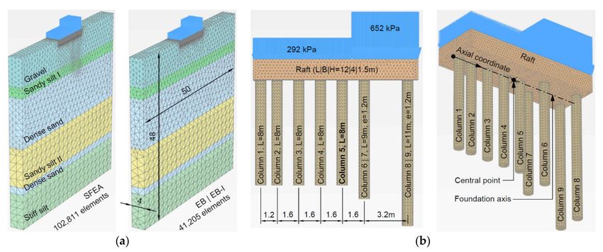
Processes 2021, 9, 1739                                                                                             2 of 27

                          the number of degrees of freedom (DOFs) increases disproportionately, resulting in com-
                          putational costs that must be regarded as unbearable for most practical purposes [13]. In
                          addition, the SFEA requires an a priori consideration of the orientation and location of
                          the piles during the geometrical setup-up of the model, which makes design optimization
                          cumbersome in engineering practice [14].
                                To overcome these limitations, Sadek and Shahrour [15] proposed the so-called em-
                          bedded beam (EB) formulation, which was further enhanced through the contributions of
                          Engin et al. [16], as well as Tschuchnigg and Schweiger [12]; in more recent publications, the
                          EB is also referred to as embedded pile [13,17]. In its actual configuration, EBs constitute
                          line elements composed of beams and non-linear embedded interface elements, allowing
                          for relative beam-soil displacements. Unlike the SFEA, the EB formulation defines piles
                          independent from the solid mesh connectivity; consequently, EBs do not influence the
                          spatial discretization of the soil domain, leading to a significant decrease in DOFs close
                          to the thin geometrical entities, higher calculation efficiency, and lower modelling effort
                          compared to the SFEA. In addition, the EB simplifies the structural analysis with respect to
                          the evaluation of stress resultants [13].
                                Since the EB modelling technique considers SSI along the centreline only, it was
                          originally intended for the analysis of axially-loaded small diameter piles installed in
                          vertical direction [18]. Due to its deficiency to capture the effect of pile installation in the
                          surrounding soil, it is further recommended to apply the EB framework for the modelling
                          of piles undergoing inconsiderable installation effects, such as non-displacement piles
                          or, more specifically, piles which are constructed using casings [12]. Applications of EBs
                          are reported for single piles under compression [19] and tension [20], pile rows [21], pile
                          groups [22,23], rigid inclusions [24], connected [25–29] and disconnected piled rafts [13].
                          Despite aforementioned recommendations regarding its field of application, and due
                          to its exceptional ability to simplify the modelling process, EBs were found eligible for
                          the modelling of almost any type of geotechnical reinforcement interacting with solid
                          elements: Abbas et al. investigated both the lateral load behaviour [30] and the uplift load-
                          carrying mechanism [31] of inclined micropiles modelled by means of EBs. El-Sherbiny
                          et al. [32] applied EBs to study the ability of jet-grout columns to stabilize berms in soft
                          soil formations. EBs found also use in the modelling of piles subjected to different modes
                          of loading, namely lateral [33], passive [34,35], and dynamic loading [36]. More recently,
                          use cases suggest the incorporation of EBs to capture the response of tension members,
                          including tunnel front fiberglass reinforcements [37], rock bolts [38], ground anchors [39],
                          and soil nails [40].
                                However, as relevant as it is poorly considered, the existing EB formulation suffers
                          from severe limitations compared to the SFEA. Most significantly, this modelling approach
                          introduces a mechanical incompatibility, resulting in stress singularities near the pile
                          base [41]. This effect is mesh-dependent and becomes more determinant with increasing
                          mesh refinement in the vicinity of an EB; accordingly, EBs require the employment of
                          sufficiently coarse mesh discretizations in order to accurately predict their system response.
                          Otherwise, increasing the mesh coarseness of the solid domain gives rise to inaccurate
                          solutions and inconvenient convergence to the sought exact solution [13]; from a practical
                          point of view, this may lead to an underestimation of foundation settlements. Hence,
                          engineering judgment, in conjunction with mesh studies, are in demand to evaluate reliable
                          mesh discretizations. Another important limiting factor concerns the SSI principle: as the
                          latter is established along the centreline rather than the physical circumference, EBs cannot
                          distinguish between lateral shear and normal stress components acting on the interface,
                          which are therefore unlimited [18]. In this way, lateral plasticity is solely controlled by the
                          evolution of failure points in the surrounding soil; this obstacle may give rise to inaccurate
                          predictions in the case of complex loading situations [42].
                                To solve aforementioned problems, Turello et al. [41,43] developed the so-called
                          embedded beam with interaction surface (EB-I). The novelty of this approach concerned
                          the integration of an explicit interaction surface to the existing EB formulation, which allows
Processes 2021, 9, 1739                                                                                            3 of 27

                          the spread of non-linear SSI effects over the physical skin, instead of over the centreline. In
                          this way, spurious stress singularities induced by the line element are markedly reduced.
                          More recently, the improved embedded beam framework was further generalized in order
                          to allow for inclined pile configurations as well as non-circular cross-section shapes [10,42].
                          Aforementioned publications found that the EB-I poses a significant enhancement, in terms
                          of mesh sensitivity and global pile response, in comparison with the original EB. However,
                          it should be noted that these papers were primarily devoted to the theoretical presentation
                          of the EB-I concept, hence little attention was paid to its validation. For example, Turello
                          et al. [44] investigated its ability to resemble pile group members considering linear elastic
                          soil conditions, which must be regarded as considerable simplification with respect to the
                          mechanical soil behaviour. Moreover, Smulders et al. [42] evaluated the EB-I performance
                          solely based on the load-settlement behaviour of single piles, which is mainly controlled
                          by the stiffness of the surrounding soil [11].
                                The present paper aims at assessing the relative merits of the improved embedded
                          beam formulation, compared to the existing one, in more detail. To this end, the remainder
                          of this paper is organized as follows: Section 2 reconsiders the theoretical framework
                          of both embedded beam formulations and highlights important differences. Section 3
                          presents the numerical modelling approach applied in the numerical studies. Section 4
                          investigates the credibility of results computed with both embedded beam formulations
                          based on a single-pile engineering case. In view of their intended use (i.e., to capture the
                          behaviour of SFEA piles; see [11]), the performance of both embedded beam formulations
                          is analysed based on a comparison with the results obtained using the SFEA, which serves
                          as a benchmark model for numerical validation [45]. In this context, it is noted that the
                          (numerical) validation approach applied differs from the traditional validation strategy [46],
                          which generally uses experimental data as a benchmark. To the authors’ knowledge, the
                          underlying studies represent the first attempt to compare the structural performance of
                          embedded beam formulations with respect to the mobilization of skin tractions, load
                          separation between pile shaft and pile base, as well as displacements induced in the
                          surrounding soil. In Section 5, both embedded beam models are utilized to approximate
                          deep foundation elements of a recently constructed railway station, but emphasis is given
                          to practical implications. Section 6 closes with the main conclusions of this work. In
                          the course of this document, boldface uppercase and lowercase letters denote vectors or
                          matrices, respectively. Italic element symbols are defined in the list of symbols.

                          2. Background
                          2.1. Embedded Beam Formulation
                              EBs combine the efficient use of defining beam elements independent of the solid mesh
                          connectivity, with slip between the structural element and the solid mesh defined along the
                          element axis. Over the last decade, many commercial software codes have incorporated an
                          EB-type element; see Table 1. Though the latter differs in terms of element type name and
                          recommended application, the working principle is broadly the same.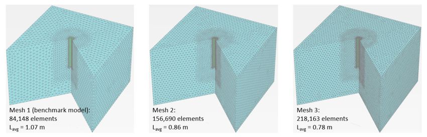
Processes 2021, 9, 1739                                                                                                                   4 of 27

                            Table 1. Overview of EB-type elements employed in numerical software codes.

          Numerical Code                   Diana 3D           ZSoil 3D                  RS3                FLAC 3D           PLAXIS 3D
             (Version)                    (V10.4) [47]      (V20.07) [48]           (V4.014) [49]         (V7.0) [50]       (V21.00) [51]
         Simulation Method                   FEM               FEM                      FEM                  FDM               FEM
                                                             Composite               Embedded            Pile structural    Embedded
             EB-type name               Pile foundations
                                                              element                 element               element        beam element
      Soil-structure interaction                              Line interface along shaft, point interface at base
  Skin resistance in axial direction                          Soil-dependent or pre-defined traction (kN/m)
  Base resistance in axial direction                                            Pre-defined force (kN)
                                                           Piles, soil nails,                              Structural
                                         Piles, ground                             Piles, forepoles,                       Piles, rockbolts,
              Application                                     fixed end                                     support
                                            anchors                                     beams                                  anchors
                                                               anchors                                     members

                                        From a numerical point of view, EBs implemented in Plaxis 3D represent composite
                                   structural elements comprising three components:

                                   1.    Three-noded beam element with quadratic interpolation scheme and six DOFs (i.e.,
                                         three translational DOFs, u x , uy , uz ; three rotational DOFs, ϕ x , ϕy , ϕz ). As Timo-
                                         shenko’s theory is adopted, shear deformations are explicitly taken into account. In
                                         order to improve the numerical stability in case of particularly fine mesh discretiza-
                                         tions, an elastic zone is automatically generated in the surrounding soil. In this zone,
                                         all Gaussian points of the solid mesh are forced to remain elastic. As the zone size is
                                         controlled by the pile radius, the geometrical properties of the beam element influence
                                         the stress state in the surrounding soil [16].
                                   2.    Three-noded line interfaces with the quadratic interpolation scheme and three pairs
                                         of nodes instead of single nodes, one belonging to the beam and one to the solid
                                         element in which the beam is located. This component accounts for the SSI along the
                                         shaft based on a material law that links the skin traction vector tskin
                                                                                                               EB (kN/m) to the
                                         relative displacement vector urel (m):

                                                                        urel = ub − us = Nb ·ab − Ns ·as                                     (1)

                                                                                    tskin  e
                                                                                     EB = D ·urel                                            (2)
                                         where ub and us (m) denote the beam and solid displacement vector, while matrices
                                         Nb and Ns represent the interpolation matrix, including standard Lagrangian element
                                         functions of the corresponding beam and solid elements. The elastic constitutive
                                         matrix De (kN/m2 ) is composed of the embedded interface stiffnesses in normal and
                                         tangential directions. Unlike the beam component, interface stiffness matrices are
                                         evaluated employing the Newton–Cotes integration scheme, hence element function
                                         values at the nodes are either one or zero. While skin traction components in radial
                                         direction are defined as unlimited, peak values in axial direction t axial,max (kN/m)
                                         may be linked to the actual soil stress state using a Coulomb criterion:

                                                                                      avg0
                                                                t axial, max ≤ c0 − σn · tan ϕ0 ·2·π · R                    (3)

                                                                                                                                   avg0
                                         where c0 (kPa) and ϕ0 (◦ ) represent the effective soil strength parameters, σn (kPa)
                                         the averaged effective normal stress along the line interface and R (m) the radius.
                                   3.    Point interface with one integration point at the beam end. In its initial configuration,
                                         the latter coincides with a solid node. Similar to the line interface, SSI effects obey a
                                         material law defined in terms of urel (m) and the embedded foot interface stiffness
                                         Kbase (kN/m) in an axial direction. On the contrary, the ultimate tip force is limited
                                         through a user-defined tip force Fmax (kN), hence independent of the surrounding
                                         soil. Tensile stresses are internally suppressed through a tension cut-off criterion.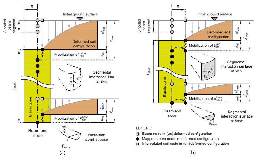
Processes 2021, 9, 1739                                                                                              5 of 27

                               For details concerning virtual work considerations and the iteration procedure, the
                          interested reader can refer to [47–51].

                          2.2. Improved Embedded Beam Formulation with Interaction Surface
                               To the best of found knowledge, the EB-I is yet to feature in commercial software codes.
                          However, recent developments have been tested and incorporated in Plaxis 3D [18,42].
                          In order to get a better understanding of the enhancements compared to the EB, a few
                          remarks on the implementation are noteworthy:

                          •   Unlike EBs, which consider shaft SSI effects along the beam axis, the EB-I spreads the
                              shaft resistance over a number of integration points located at the physical interac-
                              tion surface; the same applies for SSI at the base, where the resistance is distributed
                              over several points at the base, instead of a single point. In this way, singular stress
                              concentrations, leading to local accumulations of plastic behaviour and large displace-
                              ments along the axis, are avoided. In analogy to the EB, the skin traction vector tskin
                                                                                                                 EB−I
                              (kN/m2 ) is expressed in terms of the relative displacement vector at the interaction
                              surface urel (m) and the elastic stiffness matrix De (kN/m3 ):

                                                           urel = ub − us = H·ab − Ns ·as                               (4)

                                                                               De
                                                                  tskin
                                                                   EB−I =         ·u                                    (5)
                                                                              2πR rel
                              where ub (m) denotes the mapped beam displacement at the interaction surface
                              expressed in terms of the mapping matrix H and beam nodal DOFs ab . us (m) is the
                              solid displacement vector at the interaction surface obtained by means of interpolation,
                              within solid elements, located at the interaction surface. The latter is calculated based
                              on vector as containing solid nodal DOFs and the interpolation matrix Ns including
                              standard Lagrangian element functions of the corresponding solid elements. R (m)
                              represents the beam radius and De (kN/m2 ) represents the elastic stiffness matrix
                              containing the interface stiffnesses. Since each interface element no longer poses a
                              line, but a surface, the latter is divided by the shaft circumference. A similar approach
                              is applied to resemble SSI at the base.
                          •   In contrast to EBs, EB-Is are able to distinguish between two shear stress directions
                              perpendicular to the beam axis. This allows them to enrich the slip criterion such that
                              it accounts for any possible direction of slip failure occurring at the interaction surface:
                                                                  q
                                                         τmax =       τs2 + τt2 ≤ c0 − σn0 · tan ϕ0                     (6)

                              where τmax (kN/m2 ) is the max. local shear stress, controlled by the (perpendicularly
                              oriented) local shear stress components τs and τt (kN/m2 ) acting on the interaction
                              surface. σn0 (kN/m2 ) denotes the actual normal stress developing in the surrounding
                              soil, c0 (kN/m2 ) and ϕ0 (◦ ) the effective soil strength parameters. Accordingly, the
                              intrinsic slip criterion is not restricted to the axial direction, as is the case for the EB.
                          •   Depending on the discretization and the number of integration points at the interaction
                              surface, the EB-I connects multiple continuum elements to one beam element. From a
                              numerical point of view, the embedded beam stiffness is spread over a higher number
                              of nodes, leading to relative merits in terms of global stiffness matrix conditioning
                              (i.e., smaller difference between max. and min. diagonal terms). As a consequence,
                              the robustness of the numerical procedure is improved compared to the EB.

                               For the sake of clarity, Figure 1 compares the global response of a vertically loaded
                          single pile, modelled by means of both embedded beam formulations, namely the existing
                          embedded beam (EB) and the improved embedded beam with interaction surface (EB-I).
Processes 2021, 9, 1739                                                                                                          6 of 27

      Figure 1. Global response of an axially loaded pile, considered by means of different modelling approaches: (a) embedded
      beam (EB); (b) embedded beam with interaction surface (EB-I). In both cases, the mobilization of skin tractions is primarily
      controlled by the relative displacement vector urel (“spring”) and the slip criterion (“friction element”).

                                  3. Finite Element Modelling
                                  3.1. Investigated Scenario and Model Description
                                       Although single piles are rarely constructed in isolation, it is useful to consider their
                                  analysis for the numerical validation of new pile modelling methods [4]. Accordingly, the
                                  Alzey Bridge pile load test [52] serves as a reference scenario to compare the performance of
                                  the EB with the EB-I. The test program was originally intended to optimize the foundation
                                  design of a highway bridge in slightly overconsolidated Frankfurt clay. Recently, it has
                                  gained increasing popularity for the performance assessment of novel pile formulations;
                                  for example, see [16,42].
                                       The numerical simulations, carried out in the present study, consider different pile
                                  modelling approaches and mesh discretizations. All simulations are carried out with Plaxis
                                  3D [51]. For the sake of numerical consistency, in terms of solid element type and domain
                                  dimensions, all results are obtained using full 3D models, instead of axisymmetric 2D
                                  models or reduced 3D models for the SFEA. In view of the number of elements and DOFs
                                  required to discretize the domain, this allows for a direct comparison between SFEA and
                                  EB/EB-I models. Following the results of trial simulations, the model domain has been
                                  defined such that boundary effects are reduced to an acceptable limit; see Appendix A.
                                  Consequently, the model dimensions Bm = Lm /Dm are set to 26/19 m, which is equal to
                                  20 and 2 times the pile diameter and length, respectively; see Figure 2a. With regard to
                                  the boundary conditions, conventional kinematic conditions are considered: a fully fixed
                                  support, with blocking of the displacements in all directions, at the lower horizontal model
                                  boundary and a horizontally fixed support with freedom of vertical displacements along
                                  lateral model boundaries. Moreover, mesh sensitivity analyses, concerning the (numerical)
                                  benchmark solution, ensure that the reference model is stable and reliable; see Appendix B.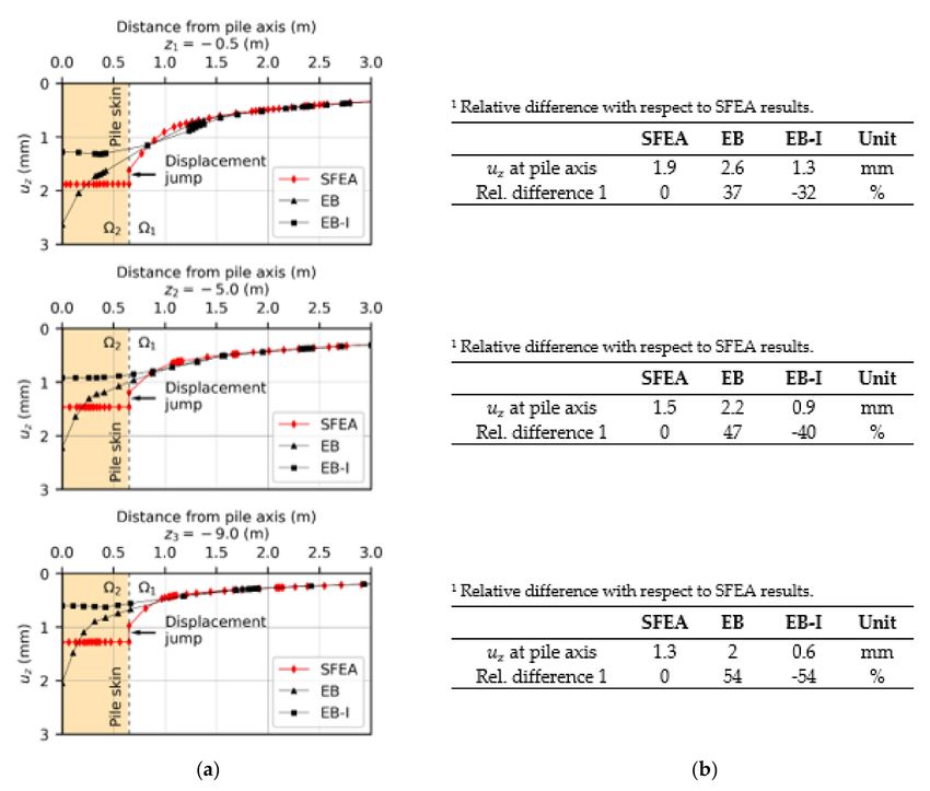
Processes 2021, 9, 1739                                                                                                7 of 27

                          Figure 2. (a) Model geometry, boundary conditions, and (b) characteristic load-displacement regions
                          after [53].

                                Regardless of the pile modelling approach, the majority of the performed finite ele-
                          ment analyses (FEA) consist of five phases. All simulations start with the definition of the
                          initial conditions, where the initial stress field is generated by means of the K0 procedure;
                          this is reasonable given a horizontal ground surface and homogeneous soil. The next phase
                          concerns the pile installation; depending on the considered pile configuration, this includes
                          the assignment of hardened concrete properties and the activation of interface elements
                          between the pile and the surrounding soil (SFEA), or the activation of the respective embed-
                          ded beam element (EB, EB-I). Hence, the piles are assumed to be homogenous in strength,
                          stiffness, and weight, thereby ignoring effects of improper concreting [6]. According to
                          the reference scenario, the soil around the pile is assumed to be in its initial state, which
                          may be regarded as reasonable for non-displacement piles, where installation effects are of
                          subordinate importance with respect to the pile behaviour [8]. Unless otherwise stated, the
                          pile is finally subjected to displacement-driven head-down loading.
                                In the course of the evaluation of results, the mesh size effect on derived quantities (for
                          example, the mobilization of skin and base resistance) is compared at different displacement
                          levels. To satisfy practical relations on the one hand, and reduce bias on the other hand,
                          the prescribed displacements are specified beforehand, following the L1-L2 method [53];
                          see Figure 2b.
                                Assuming drained conditions, the following prescribed displacements are determined
                          as a function of the pile diameter DPile :

                          •    u L1 = uPile /DPile = 0.34%, approximating the end of the initial linear region [54].
                          •    u L2 = uPile /DPile = 4%, indicating the initiation of the final linear region [55].
                          •    uult = uPile /DPile = 10%, complying with the ultimate pile resistance defined in [56].

                               As shown in Figure 2b, u L1 and u L2 correspond to the pile head displacement uPile at
                          the end of the initial linear region, as well as at the initiation of the final linear region. uult
                          marks the pile head displacement at the end of loading.

                          3.2. Pile Modelling Approach
                               As suggested by [10,38,41], the numerical behaviour of embedded beam formulations
                          is numerically validated against SFEA results (i.e., full 3D FE model). In the latter case,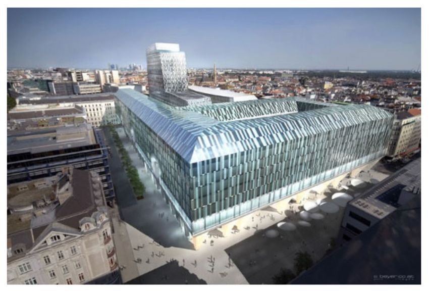
Processes 2021, 9, 1739                                                                                              8 of 27

                          the swept meshing technique [57] is applied to discretize the domain with 84,148 10-
                          noded tetrahedral elements. In this way, the solid elements representing the SFEA pile
                          are discretized with a structured swept mesh, allowing for both a faster mesh generation
                          process, as well as a considerable mesh size reduction compared to the default solid mesh.
                                In order to minimize the interpolation error associated with the mesh discretization of
                          the model, the mesh is refined inside the pile structure, and within a zone of 3·DPile below
                          the tip and beside the shaft, respectively; see Figure 3. To address possible occurrence of
                          relative displacements and plastic slip parallel to the soil-structure contacts, standard zero-
                          thickness interface elements are considered at soil-structure contacts [58,59]. The interface
                          elements are extended beyond the physical pile boundary in order to reduce the effect of
                          singular plasticity points developing close to the pile edge [11,60]. The interface strength is
                          specified with a Coulomb criterion that limits the max. shear stress τ max (kN/m2 ) by

                                                          τ max = c0 − σn0 · tan ϕ0 · Rinter

                                                                                                                      (7)

                          where σn0 (kN/m2 ), ϕ0 (◦ ), and c0 (kN/m2 ) are the effective interface normal stress, interface
                          friction angle, and interface cohesion. In accordance with recommendations given in [61],
                          an interface reduction factor Rinter = 0.9 is adopted in the analyses, which represents a
                          typical value to account for SSI between concrete piles and fine grained soils.

                          Figure 3. (a) 3D view of global SFEA mesh; (b) cross-sectional view of SFEA mesh detail.

                                Contrary to SFEA interfaces, embedded interface elements are not explicitly modelled,
                          but they are internally defined after the global mesh discretization; thus, assigning interface
                          parameters reduces the definition of the ultimate skin and base resistance. For the sake of
                          numerical consistency, the skin resistance is defined as layer-dependent (i.e., dependent
                          of the stress state in the surrounding soil; see Equation (3)). In this way, the embedded
                          interface elements are defined similarly to the interface elements used in the SFEA [12]. In
                          an attempt to capture the SFEA pile capacity with sufficient accuracy, the base resistance
                          is limited by the SFEA normal force developing at the pile base after the final loading
                          step. The mesh sensitivity of both embedded beam formulations is investigated with
                          five different mesh refinements, which are referred to as very fine, fine, medium, coarse,
                          and very coarse (Figure 4). The model boundary conditions are specified equal to the
                          SFEA case.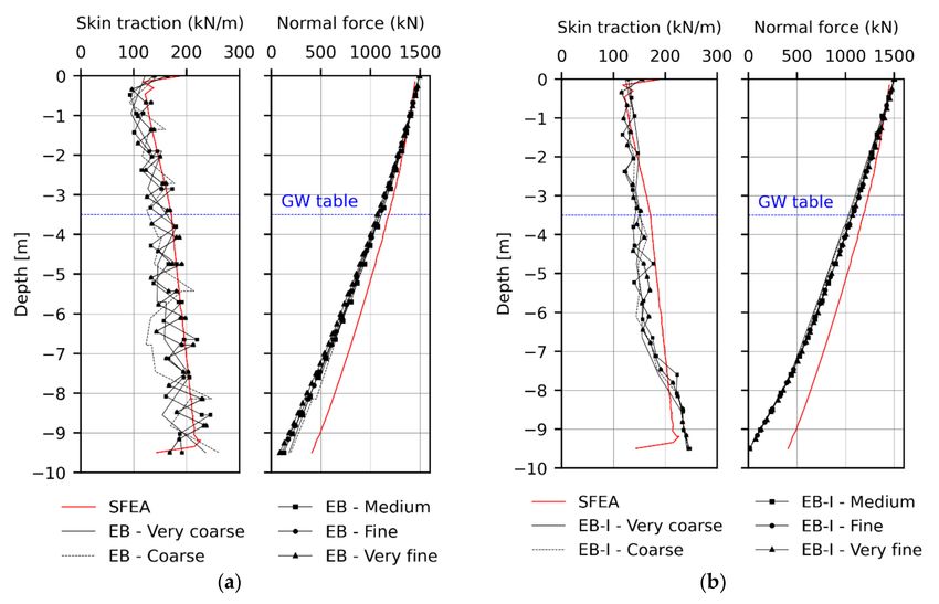
Processes 2021, 9, 1739                                                                                                    9 of 27

                              Figure 4. Mesh discretizations considered for EB/EB-I models.

                               It is noted that both embedded beam formulations are analysed with the same mesh
                          discretizations and considerably less DOFs compared to the SFEA. Since beam elements are
                          superimposed on the solid domain, and therefore overlap the soil, the beam unit weight
                          represents a delta unit weight to the surrounding soil [11]. Noteworthy, this differs from
                          previous interpretations of the embedded beam unit weight documented in [27,30,31,62],
                          where the unit weight is assigned with the actual unit weight of the volume pile; as a
                          consequence, this approach leads to an overestimation of the soil-structure unit weight.
                          To realistically approximate the kinematics at the pile head, the uppermost connection
                          point is considered as free to move and rotate, relative to the surrounding soil. Additional
                          modelling parameters summarized in Table 2 are taken from [16] and resemble on-site
                          conditions as described in [52].

                          Table 2. Overview of pile parameters applied in the Alzey Bridge model.

                                       Parameter              Symbol           Unit          SFEA              EB/EB-I 1
                                                                                      Pile      Interface    Pile    Interface
                                      Unit weight                 γ        kN/m3      25.0                    5.0
                                   Young’s modulus                E         GPa       10.0                   10.0
                                     Poisson’s ratio              ν          -         0.2
                                      Pile diameter               D          m         1.3                   1.3
                                       Pile length                L          m         9.5                   9.5
                                     Base resistance            Fmax        kN                              2300.0
                               Interface reduction factor       Rinter       -                       0.9                0.9
                                Effective friction angle         ϕ0         deg                     20.0               20.0
                                   Effective cohesion            c0        kN/m2                    20.0               20.0
                          1   Calibrated numerical model documented in [18].

                          3.3. Constitutive Model and Parameter Determination
                                Regardless of the pile modelling approach, the use of a proper constitutive model
                          is crucial to cover the complex stress-strain behaviour of soils. Specific to this study, this
                          includes a realistic evolution of potential slip planes along the pile-soil contacts, which is
                          fundamental in the analysis of the pile behaviour. Since piles may undergo a wide range
                          of deformations, leading to considerable strains in the soil, the constitutive model should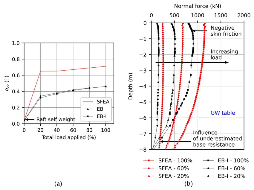
Processes 2021, 9, 1739                                                                                          10 of 27

                          also be capable of effectively simulating the shear modulus degradation with the evolution
                          of shear strain [63]. Lastly, the constitutive model is supposed to account for the stress
                          dependency of soil stiffness in order to capture the gradual mobilization of skin friction
                          with sufficient accuracy [11].
                                Concerning these critical modelling aspects, the Hardening Soil Small (HSS) with non-
                          associated flow rule and small-strain stiffness overlay [64], an extension of the Hardening
                          Soil (HS) model [65], is used in this study. While HS parameters and drainage conditions are
                          adopted from [16], HSS-specific model parameters, namely the threshold shear strain for
                          stiffness degradation, γ0.7 , and the initial shear modulus, G0 , are defined using empirical
                          correlations documented in [66] and [67], respectively. The groundwater table is located
                          3.5 m below ground surface. Soil parameters adopted in the analyses are listed in Table 3.

                          Table 3. Overview of soil parameters applied in Alzey Bridge model.

                                              Parameter                          Symbol         Unit         Value
                                        Drainage conditions                        -              -         drained
                                    Depth of groundwater table                     -              m            3.5
                                            Unit weight                      γsat ,γunsat       kN/m3         20.0
                                                                                   re f
                           Reference deviatoric hardening modulus at pref         E50           kN/m2        45,000
                                                                                   re f
                                Reference oedometer stiffness at pref             Eoed          kN/m2        27,150
                                                                                   re f
                               Reference un-/reloading stiffness at pref          Eur           kN/m2        90,000
                                              Power index                           m             -            1.0
                                       Isotropic Poisson’s ratio                     0
                                                                                   νur            -            0.2
                                        Effective friction angle                   ϕ0            deg           20.0
                                           Effective cohesion                       c0          kN/m2         20.0
                                       Pre-overburden pressure                    POP           kN/m2         50.0
                                          Reference pressure                      pre f         kN/m2         100.0
                                                                                    re f
                                     Initial shear modulus at pref                G0            kN/m2       116,000
                                        Threshold shear strain                    γ0.7            -         0.00015

                          4. Numerical Validation
                               A series of finite element analyses has been performed to assess the performance of the
                          improved embedded beam with interaction surface. Therefore, the latter is compared to the
                          existing embedded beam formulation, as well as the SFEA, which serves as the benchmark.
                          The simulations focus on two specific points: mesh sensitivity studies and displacements
                          induced in the surrounding soil. In addition, practical implications are drawn based on
                          the results.

                          4.1. Influence of Mesh Size on Global Pile Behaviour
                                The most critical issue in the design of pile supported structures is a reliable predic-
                          tion of the pile behaviour, in terms of bearing capacity and settlement, under working
                          load conditions [68]. Consequently, the first series of calculations has been performed to
                          investigate the mesh size effect on the mobilization of compressive pile resistance Rc (kN).
                                As it can be observed in Figure 5, all pile models show a similar behaviour in the first
                          stage of loading, regardless of spatial discretization level and pile modelling approach.
                          However, as the load increases beyond 2000 kN, the results reveal considerable limitations
                          of the EB, including a significant scatter of results and overestimation of bearing capacity,
                          compared to the reference solution. Although it is generally known that coarser meshes
                          yield a stiffer pile response, the wide scatter of load-displacement curves must be regarded
                          as considerable obstacles to produce consistent results. In contrast, a more realistic pile
                          response is obtained when employing the EB-I, thereby transforming the pile-soil line in-
                          terface to an explicit interaction surface. Up to a relative displacement of 2%, the mobilized
                          pile resistance magnitudes are almost independent of the domain discretization. Even at
                          higher displacement levels, the mesh size effect remains insignificant compared to the EB.
Processes 2021, 9, 1739 11 of 27
Figure 5. Influence of spatial discretization on mobilization of compressive pile resistance.
In view of the load-displacement behaviour, the EB-I gives a softer global response
compared to the EB after reaching the ultimate skin resistance, which is mainly attributed
to the different mobilization of base resistance Rb (kN); see Figure 6. The base–resistance
curves, deduced from both embedded beam formulations, may be well approximated
through bi-linear functions bounded by the max. base resistance Fmax , which is a direct
input to the analysis. However, the EB shows considerably steeper gradients in comparison
with the EB-I, which is a direct consequence of the modified embedded base interface
stiffness considered in the actual EB-I configuration. As a by-product, EB-I curves are in
remarkable agreement with the reference solution. Moreover, the results confirm that the
EB-I is less mesh-size dependent; for example, at a relative displacement of 2%, the range
of Rc -values obtained with the EB-I (1000 kN). Nevertheless, both formulations have deficiencies regarding the
initial mobilization of base resistance in the first part of loading (see Figure 6); in all
cases considered, the base resistance is considerably underestimated and shows a lower
mobilization rate compared to the SFEA. This must be regarded as a considerable limitation
of the actual embedded beam configurations.
Figure 6. Influence of spatial discretization on the mobilization of base resistance.
Figure 7 provides more insight into the effect of different mesh discretizations on
the mobilization of Rc at different pile displacement levels, namely u L1 , u L2 , and uult ; see
Figure 2b. The obtained Rc -values are normalized with respect to the benchmark solution:
Rc,EB| EB− I
Rc,norm = ·100 % (8)
Rc,SFEAProcesses 2021, 9, 1739 12 of 27
where Rc,norm (%) is the normalized compressive pile resistance. Rc,EB| EB− I (kN) and
Rc,SFEA (kN) represent the mobilized compressive pile resistance, either obtained with the
EB, EB-I, or SFEA at a given pile head displacement. To quantify the refinement level of
the considered mesh, independent of the model dimensions, the results are plotted versus
the average element size L avg (m), which is internally controlled by the mesh coarseness
factor and the model dimensions [57].
Figure 7. Influence of spatial discretization on the mobilization of pile resistance at different displacement levels, namely
(a) u L1 , (b) u L2 , (c) urel .
In compliance with the previous results, the EB-I achieves a satisfactory agreement
with the reference solution, with the max. deviation being as little as 12%. On the contrary,
Rc -magnitudes obtained with the EB are highly mesh-dependent. In all cases considered,
the EB yields the highest Rc -values. In particular, for coarse mesh discretizations, the
benchmark value is considerably overestimated with a peak deviation of 58%.
In order to describe the mesh size effect by means of a quantitative measure, the mesh
dependency ratio MDR is introduced:
Rc,max
MDR = ≥ 1.0 (9)
Rc,min
where Rc,max and Rc,min (kN) represent the max. and min. compressive pile resistance
values obtained at a given pile head displacement, either using the EB or the EB-I. Obviously,
a MDR of 1.0 indicates mesh-independency, even though the results may differ from the
reference solution. As expected, MDR-values listed in Table 4 are remarkably smaller
for the EB-I, thus underlining that the EB-I is clearly superior in the elimination of the
mesh-size effect for all cases considered. For example, at the pile head displacement of u L1 ,
the MDR reduces to 1.02 for the EB-I; at the other extreme, the MDR gives 1.22 for the EB.
Table 4. Summary of pile resistance values obtained at different displacement levels.
Lavg EB EB-I
Mesh Configuration Unit
m Rc, uL1 Rc, uL2 Rc, uult Rc, uL1 Rc, uL2 Rc, uult
Very coarse 4.15 2355 4642 4667 1867 3284 3855 kN
Coarse 3.44 2363 4386 4385 1877 3208 3876 kN
Medium 2.48 2045 4224 4208 1887 3017 3863 kN
Fine 1.81 1974 3723 3975 1891 3283 3916 kN
Very Fine 1.32 1940 3603 4228 1906 3071 3796 kN
MDR 1.22 1.29 1.17 1.02 1.09 1.03 -Processes 2021, 9, 1739 13 of 27
4.2. Influence of Mesh Size on Pile Load Transfer Mechanism
A realistic representation of the load sharing between pile shaft and pile base is critical
in the analysis of geotechnical structures, including deep foundation elements. For example,
Zhou et al. [69] have reported that the development of differential settlements, developing
between the pile and surrounding soil, is more pronounced for end-bearing piles, in
comparison with floating piles. In addition, the load-carrying mechanism influences the
development of skin tractions along the pile length, hence, this is of paramount importance
in the analysis of composite foundations such as piled rafts [70]. As discussed in Section 1,
these structures are often modelled using EB, although the load transfer mechanism has
been rarely validated in literature.
To close this knowledge gap, a closer inspection of the load separation is given in
Figure 8, where relative pile head displacements are plotted versus skin resistance ratios
(i.e., percentage of total load resisted by skin friction). This approach is often utilized to
characterize the load-bearing behaviour of piles, whereas admissible values range from 0%
(end-bearing pile) to 100% (floating pile). In all cases considered, the results infer that the
skin resistance ratio decreases with increasing pile displacement, albeit underestimated, at
around 20%, in the initial stage of loading. While all curves obtained with the EB-I converge
to the reference solution at approximately 40%, the EB indicates mesh sensitive values that
vary within higher bounds. This observation complies with previous findings concerning
Rc [42]; as the ultimate base resistance is limited by Fmax , the scatter of magnitudes must be
caused by an overestimation of the skin resistance. This tendency, in turn, is presumably
triggered by singular skin traction values developing near the pile base, which are likely to
occur due to a combination of very high stress gradients in the soil elements around the pile
base and constitutive models concerning stress-dependent soil stiffness; a comprehensive
discussion on this limitation inherent to EBs is provided in [11].
Figure 8. Influence of spatial discretization on load separation plotted by means of skin resistance ratio.
4.3. Influence of Mesh Size on Pile Stiffness Coefficient
In traditional serviceability analysis of pile-plate systems, SSI effects are numerically
considered as spring constants acting on bending plates [56]. In this context, the pile
stiffness coefficient k s (MN/m), representing the pile stiffness, is expressed by the formula:
Rc,i
ks = (10)
ui
where Rc,i (kN) is the compressive pile resistance, mobilized at the pile head displacement
ui (mm). The current engineering approach assumes k s from the secant on the resistance-
settlement curve of pile load tests working in the initial linear region, commonly adopting
empirical data with respect to allowable settlements [69]. Following engineering practice,
k s is calculated as the slope of the secant line connecting the origin to the curve at u L2 ; seeProcesses 2021, 9, 1739 14 of 27
Figure 3b. Figure 9a presents k s -values as a function of L avg ; in analogy to Equation (8),
derived quantities are normalized with respect to the benchmark solution. As one can
observe, all EB-I results are in remarkable agreement with the benchmark solution; on the
contrary, the EB overestimates k s up to 26%. With regard to the mesh dependency ratio,
the EB-I yields values that are too small to warrant differentiation, while the EB, again,
indicates a notable mesh sensitivity; see Figure 9b. From a practical point of view, the EB-I
increases the confidence with which k s may be estimated by reducing the influence of the
mesh size.
Figure 9. Mesh size effect on (a) normalized pile stiffness factor and (b) respective mesh dependency ratio.
4.4. Influence of Mesh Size on Mobilization of Skin Traction
Many researchers have focused on the evaluation of normal forces to study the load-
transfer mechanism of EB along the pile length (for example, see [13,24,37]). Skin traction
profiles, in contrast, have received only subordinate attention. The underlying cause
becomes apparent from Figure 10, which compares both approaches at typical working
load conditions. Regardless of the pile modelling approach, the normal force distribution
indicates a smooth distribution of skin tractions along the pile length. In comparison with
the reference solution, increasing deviations towards the pile base are attributed to the
spurious mobilization of base resistance, which is underestimated with the EB and EB-I in
the initial stage of loading; see Section 4.1.
In contrast, the EB yields numerical oscillations in the predicted skin traction response
for all mesh discretizations considered, even though the mean values are almost identical
to the benchmark results. To explain the origin for this abnormality, the following points
deserve attention:
• EB results of the beam and the line interface are presented at the nodes [71]. Therefore,
the normal forces are internally extrapolated from Gaussian beam stress points to
the node of interest, leading to smooth profiles. In contrast, Equation (2) is used
to work out nodal skin tractions, which are consequently a function of the relative
displacement vector field and the embedded stiffness matrix. An additional parametric
study (not shown) has revealed that skin traction oscillations also occur with linear
elastic soil behaviour, ensuring identical (stress-independent) embedded stiffness
values along the pile length. Consequently, the apparent reasoning of the oscillations
must be attributed to the relative displacement vector field, which is interpolated
using displacement vector fields of different continuity at the element boundaries (C0
for soil displacements; C1 for beam displacements).
• The spurious tendency to produce oscillations is amplified by high stress and strain
gradients, predominantly occurring at the EB axis. Since the EB-I evaluates the relative
displacements at multiple points over the real pile perimeter, instead of one point
located at the pile axis, local effects are significantly reduced. As a consequence, skin
traction profiles are considerably smoothened.Processes 2021, 9, 1739 15 of 27
• Oscillations of integration point stresses, observed with the SFEA, are caused by steep
stress gradients at the pile ends. This was already explained in [58].
In view of skin traction analysis, previous observations demonstrate that the EB-I
poses a significant enhancement compared to the EB, as it significantly reduces numerical
inconsistencies leading to unrealistic oscillations in skin traction.
Figure 10. Influence of mesh size on development of skin traction and normal force distribution in an axial direction at a
vertical load of 1500 kN: (a) EB, (b) EB-I.
4.5. Displacements Induced in Surronding Soil
In design situations, where the cost-effectiveness of pile caps are of primary interest,
pile spacings should be kept as close as possible [68]. The optimal pile layout, however,
should also ensure the effectiveness of resisting piles, which is primarily achieved through
sufficiently large pile spacings [72]. The assessment of optimal pile spacings may be
based on the evaluation of settlement profiles at different pile depths [52]. Moreover,
mixed foundations, involving deep foundation elements, must satisfy serviceability limits,
defined in terms of admissible differential settlements [73]. In any of these cases, it is
important to realistically capture spatial soil displacements induced by external loads. An
insight into the predicted displacement behaviour can be gained by looking at Figure 11,
where the final distribution of soil settlements, induced by a vertical load of 1500 kN, are
illustrated. At a first glance, it can be observed that:
• Except for the displacement field in close proximity to the pile base, all calculations
yield similar results within the soil domain (i.e., zone Ω1 ).
• Apparently, the pile domain (i.e., zone Ω2 ) experiences settlement concentrations,
which are particularly pronounced for the EB. This is a direct consequence of the
SSI considered along a line, thereby introducing high displacement gradients in a
radial direction. In contrast, the EB-I finds homogenous displacement regions of lower
magnitude enclosed by the explicit interaction surface; although vertical displacements
are slightly underestimated compared to the SFEA, the EB-I is obviously superior to
the EB with regard to the prediction of the general deformation pattern inside Ω2 .
A closer inspection of the settlement profiles, at different pile depths, reveals the
apparent origin of previous observations (see Figure 12): With the SFEA, an explicit
interface (i.e., series of linked pairs of nodes) is inserted at the physical pile-soil contact. ThisProcesses 2021, 9, 1739 16 of 27
interface fulfils the role of a kinematic discontinuity, capable of accounting for extremely
high strain gradients [74]. Concerning both embedded beam formulations, the fallacy
to account for the displacement jump at the pile skin becomes obvious. This is due to
the implicit nature of the embedded interface, where displacement jumps are internally
considered to describe the nodal connectivity of beam and soil nodes, but do not evolve in
the physical mesh.
Figure 11. Settlement contour plots at a vertical load of 1500 kN: (a) SFEA, (b) EB, (c) EB-I. The latter models are obtained
with the fine mesh configuration. The real pile skin is indicated by dashed lines.
Figure 12. (a) Settlement profiles and (b) vertical settlements at the pile axis, obtained with a vertical load of 1500 kN at
different pile depths.Processes 2021, 9, 1739 17 of 27
From an engineering perspective, the settlement curves evolving outside the pile
domain vary within acceptable bounds; at a distance greater than two times the pile
diameter, the settlement profiles of all pile modelling approaches practically coincide. On
the contrary, increasing deviations are observed towards the pile axis. While the EB tends
to overestimate the settlements, the EB-I gives lower values. In all cases considered, peak
deviations are observed at the lowermost settlement profile (EB: −54%, EB-I: 54%). Further
improvements of the spatial deformation behaviour are mainly related to the stiffness
definition of the embedded interface, which is at the forefront of ongoing research.
5. Case Study
As part of the restructuring of the Vienna rail node, Tschuchnigg [11] has described
the application of 3D finite element simulations to the foundation design of central station
“Wien Mitte”; see Figure 13. Due to serviceability requirements, critical zones of the
existing slab are supported by jet-grout columns to satisfy serviceability criterions, mainly
concerning differential settlements.
Figure 13. Project overview “Wien Mitte”.
The performance of previously described embedded beam formulations is assessed by
performing the same numerical simulations. In absence of measurement data, the results
are, again, numerically validated against a full 3D representation of the problem including
SFEA, which is widely recognized as convenient for the numerical analysis of similar
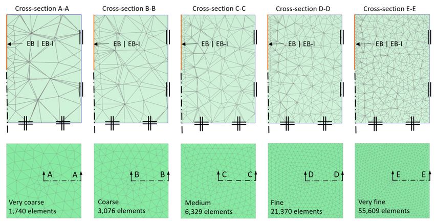
problems; for example, see [75,76]. By taking advantage of the symmetry, the model size is
defined as 50 × 4 × 48 m; see Figure 14a. The soil layering is similar to the real project. The
raft of the simplified model is supported by nine jet-grout columns, which are symmetri-
cally arranged on the foundation axis; see Figure 14b. SSI between soil and raft boundaries
are addressed by means of zero-thickness interface elements [58,59] (not shown). The base
model boundary condition is defined as fully fixed, whereas the vertical boundaries are set
to allow vertical movement of soil layers (i.e., roller supports). Depending on the column
modelling approach, the domain is discretized with 102,811 (SFEA) and 41,205 (EB, EB-I)
10-noded tetrahedral elements with quadratic element function.
Table 5 gives the HSS soil parameters adopted in the analyses; in analogy to Section 3.3,
HSS-specific soil parameters are obtained using profound empirical correlations [66,67].
Additional material parameters related to the column-raft system, as well as the calculation
phase sequence, are described in [11].Processes 2021, 9, 1739 18 of 27
Figure 14. Description of the FE analysis model “Wien Mitte”: (a) Model configuration and (b) side/3D view of
pile-raft system.
Table 5. Overview of HSS soil parameters used in the analyses (Wien Mitte).
Sandy
Parameter Symbol Unit Gravel Sand Stiff Silt
Silt I|II
Depth of groundwater table - m 6.0 - - -
Layer thickness t m 8.0 3.0|11.0 14.0|2.0 10.0
Unit weight γsat , γunsat kN/m3 21.5|21.0 20.0 21.0|20.0 20.0
re f
Reference deviatoric hardening modulus at pref E50 kN/m2 40,000 20,000 25,000 30,000
re f
Reference oedometer stiffness at pref Eoed kN/m2 40,000 20,000 25,000 30,000
re f
Reference un-/reloading stiffness at pref Eur kN/m2 120,000 50,000 62,500 90,000
Power index m - 0.0 0.8 0.65 0.6
Isotropic Poisson’s ratio 0
νur - 0.2 0.2 0.2 0.2
Effective friction angle ϕ0 deg 35.0 27.5 32.5 27.5
Effective cohesion c0 kN/m2 0.1 20.0|30.0 5.0 30.0
Ultimate dilatancy angle Ψ deg 5.0 0.0 2.5 0.0
Pre-overburden pressure POP kN/m2 600 600 600 600
Reference pressure pre f kN/m2 100 100 100 100
re f
Initial shear modulus at pref G0 kN/m2 138,000 81,000 93,000 116,000
Threshold shear strain γ0.7 - 0.00015 0.00015 0.00015 0.00015
Figure 15a compares the load-settlement curves, obtained with the embedded beam
models, against the benchmark solution. It is interesting to note that settlements occurring
at the central point (see Figure 14) are practically coincident (Processes 2021, 9, 1739 19 of 27
design of the raft) and thus, require discussion. In the simulations, all column-raft contacts
are imposed with a rigid connection. While the reference solution spreads the column-raft
interaction over multiple nodes, both embedded beam formulations consider the column-
raft connection at one node only. As the raft is discretized with solid elements occupying
no rotational DOFs, the connection type reduces to a hinge for single-node connections,
which has a remarkable influence on the magnitude of the tangent rotation developing in
direction of the foundation axis.
Figure 15. (a) Central point settlement plotted as a function of total load applied and (b) settlement curve along the
foundation axis at final load, obtained with SFEA, EB, and EB-I.
Figure 16. (a) Foundation movement at peak load and (b) schematic illustration of deformation patterns obtained with
different column modelling approaches.
Figure 16b illustrates the observed deformation patterns schematically. In the reference
model, the tangent rotation achieves max. values outside the column-raft contacts, indicat-
ing offsets between the columns. Since the tangent rotations are purely negative in sign, the
tangent between successive nodes (in direction of the axial coordinate) points strictly down-
wards. In contrast, tangent rotation peak values evolve at the column-raft contacts with
the EB and EB-I. In addition, the tangent rotations vary in sign at the column-raft contacts,
indicating relatively high curvatures. Taking into account the bending moment–curvature
relationship, this is likely to result in the spurious prediction of internal forces and an
inconvenient raft design. To circumvent these obstacles, a more realistic representation of
foundation movement could be realized by using alternative modelling techniques such
as the hybrid modelling approach described by Lődör and Balázs [24], where embedded
beams are circumscribed by volume elements at connection areas.Processes 2021, 9, 1739 20 of 27
The last section is devoted to examining the load sharing between members of the
composite geotechnical structure. In this context, the column raft coefficient αcr at different
loading stages is calculated as:
∑ Rcolumn
αcr = (11)
Rtotal
where ∑ Rcolumn (kN) defines the sum of loads carried by the columns and Rtotal (kN)
the total load applied. Figure 17a depicts αcr as a function of relative load applied. All
models show higher αcr -values with increasing load level, indicating that additional load
portions are predominantly carried by the columns. On the one hand, both embedded
beam formulations show almost identical results and converge to αcr = 0.46 after the final
stage of loading. On the other hand, deviations compared to the benchmark are striking
(αcr = 0.71) and require discussion.
Figure 17. (a) Column raft coefficient and (b) normal force distribution developing along column 5,
plotted as a function of total load applied.
To study the load transfer characteristics in more detail, Figure 17b shows the normal
force distribution along (central) column 5. Obviously, arising differences with regard to
αcr can be attributed to a combination of remaining issues associated with both embedded
beam configurations, namely:
• At load levels, fairly below the ultimate skin resistance, the load carried by the base
resistance is significantly underestimated; see Section 4.1. As a consequence, the
general column response is too soft.
• The single-node connection causes a combination of unrealistic settlement concentra-
tions and spurious stress path evolutions in the vicinity of column-raft contacts. As
a result, column 5 experiences negative skin friction along the upper portion of the
shaft (normal force increases up to a depth of around 1.0 m), instead of a direct pile
head load. As a consequence, lower αcr -values are obtained.
More research, with the aim of analysing complex boundary value problems, is part
of ongoing research.Processes 2021, 9, 1739 21 of 27
6. Discussion and Conclusions
Two different embedded beam formulations for finite element modelling of deep foun-
dation elements have been extensively compared in terms of geotechnical and structural
performance, namely the embedded beam element (EB) and the recently developed em-
bedded beam element with interaction surface (EB-I). Derived quantities are numerically
validated against the widely accepted standard FE approach (SFEA), a full 3D representa-
tion of respective structures. To the authors’ knowledge, this work poses the first attempt
to assess the suitability of the EB-I for practical use. In this respect, a number of critical
aspects have been tackled, such as load sharing between base and shaft, evolution of soil
displacements in the surrounding soil, and mobilization of skin resistance. In this context,
particular emphasis has been given to the influence of the mesh sensitivity of results. The
following conclusions are drawn from the FEA of deep foundation elements:
• In the initial phase of loading, both embedded beam formulations yield load-displacement
responses which are in remarkable agreement with the SFEA. At load levels beyond the
shaft capacity, load-displacement curves obtained with the EB are considerably mesh
sensitive, whereas the pile behaves stiffer with increasing mesh-coarseness. The EB-I,
in contrast, reduces the mesh size effect tremendously. Moreover, the EB-I achieves a
satisfactory agreement with the SFEA.
• Concerning the predicted pile capacity, the EB produces a wide scatter of results which
must be regarded as unsatisfactory. This shortcoming is effectively eliminated by
the EB-I; in all cases considered, the pile capacity varies, within acceptable bounds,
slightly higher than the SFEA target value. Reducing the mesh size effect also allows
engineers to deduce pile stiffness coefficients with more confidence.
• At typical working load conditions, skin traction profiles obtained with both embed-
ded beam formulations fit SFEA results qualitatively well. However, the EB produces
numerical oscillations about the mean that are significantly reduced with the EB-I.
• Although both embedded beam formulations appear to capture the evolution of
spatial soil displacements with sufficient accuracy, major differences occur inside the
pile domain. While the EB calculates the highest soil displacement at the pile axis, the
EB-I computes almost constant displacement profiles within the pile boundaries, as is
the case with the SFEA. However, reproducing displacement jumps at the pile skin
lies beyond the capabilities of the actual EB-I configuration.
• When modelling deep foundation elements of composite structures, by means of
embedded beams, the connection of the individual structures needs to be considered
carefully: specifically, if embedded beams are imposed with a rigid connection. Oth-
erwise, the prediction of structural forces, shaft-base load sharing, and differential
settlements may lack physical meaning.
Considering the above findings, the EB-I proves superior to the EB. Nevertheless,
several limitation of the current version have been observed which require further research
effort. This includes the development of a generally applicable concept capable of pre-
dicting SSI effects at the base with sufficient accuracy; in addition, guidelines concerning
the definition of the ultimate base resistance are still in demand. Further, future studies
should explore whether the elastic zone approach is still required with the EB-I. In the
course of this paper, the application of EB-Is was limited to axial loading cases, neglecting
passive, as well as lateral, loading; therefore, future studies should focus on more complex
loading situations, whereas the credibility of results should be carefully validated using
measurement data. Research to resolve remaining issues is ongoing with promising results
so far.
Author Contributions: A.-N.G. focused on the conceptualization, methodology, software, investiga-
tion, writing of the original draft preparation, formal analysis, and the visualization. F.T. pursued the
supervision, editing of the original draft and the project administration. All authors have read and
agreed to the published version of the manuscript.You can also read