MultiVERSE: a multiplex and multiplex-heterogeneous network embedding approach - arXiv.org
←
→
Page content transcription
If your browser does not render page correctly, please read the page content below
MultiVERSE:
                                                    a multiplex and multiplex-heterogeneous network
                                                                  embedding approach

                                            Léo Pio-Lopez1 , Alberto Valdeolivas2 , Laurent Tichit1 , Élisabeth Remy1 , and
                                                                           Anaı̈s Baudot3,4
                                                          1
                                                           Aix Marseille Univ, CNRS, Centrale Marseille, I2M, Marseille, France
                                                2
                                                    Heidelberg University, Institute for Computational Biomedicine, Heidelberg, Germany
arXiv:2008.10085v2 [cs.LG] 5 Jan 2021

                                                              3
                                                                Aix Marseille Univ, INSERM, CNRS, MMG, Marseille, France
                                                                    4
                                                                      Barcelona Supercomputing Center, Barcelona, Spain

                                                                                        Abstract
                                                   Network embedding approaches are gaining momentum to analyse a large variety of
                                              networks. Indeed, these approaches have demonstrated their efficiency through tasks such as
                                              community detection, node classification, and link prediction. However, very few network
                                              embedding methods have been specifically designed to handle multiplex networks, i.e. net-
                                              works composed of different layers sharing the same set of nodes but having different types of
                                              edges. Moreover, to our knowledge, existing approaches cannot embed multiple nodes from
                                              multiplex-heterogeneous networks, i.e. networks composed of several multiplex networks
                                              containing both different types of nodes and edges.
                                                   In this study, we propose MultiVERSE, an extension of the VERSE framework using
                                              Random Walks with Restart on Multiplex (RWR-M) and Multiplex-Heterogeneous (RWR-
                                              MH) networks. MultiVERSE is a fast and scalable method to learn node embeddings from
                                              multiplex and multiplex-heterogeneous networks.
                                                   We evaluate MultiVERSE on several biological and social networks and demonstrate
                                              its efficiency. MultiVERSE indeed outperforms most of the other methods in the tasks of
                                              link prediction and network reconstruction for multiplex network embedding, and is also
                                              efficient in link prediction for multiplex-heterogeneous network embedding. Finally, we apply
                                              MultiVERSE to study rare disease-gene associations using link prediction and clustering.

                                                    MultiVERSE is freely available on github at https://github.com/Lpiol/MultiVERSE.

                                           Keywords — network biology, multi-layer networks, multiplex networks, heterogeneous
                                        networks, machine learning, network embedding, random walks

                                        1     Introduction
                                        Networks are powerful representations to describe, visualize, and analyse complex systems in
                                        many domains. Recently, machine learning techniques started to be used on networks, but these
                                        techniques have been developed for vector data and cannot be directly applied. A major challenge
                                        thus pertains to the encoding of high-dimensional graph-based data into a feature vector. Network
                                        embedding (also known as graph representation learning) provides a solution to this challenge
                                        and allows opening the complete machine learning toolbox for network analysis.
                                            The high efficiency of network embedding approaches has been demonstrated in a wide range
                                        of applications such as community detection, node classification, or link prediction. Moreover,
                                        network embedding can leverage massive graphs, with millions of nodes [39]. Thus, with the

                                                                                            1
explosion of big data, network embeddings have been used to study many different networks,
such as social [52], neuronal [57] and molecular networks [66].
    So far, network embedding approaches have been mainly applied to monoplex networks (i.e.
single networks composed of one type of nodes and edges) [69, 35, 39]. Current technological
advances however generate a large spectrum of data, which form large heterogeneous datasets. By
design, monoplex networks are not suited to represent such diversity and complexity. Multi-layer
networks, including multiplex [46] and multiplex-heterogeneous [87] networks have been proposed
to handle these more complex but richer heterogeneous interaction datasets.
    Multiplex networks are composed of several layers, each layer being a monoplex network. All
the layers share the same set of nodes, but their edges belong to different categories (Figure
1A). Multiplex representation is pertinent to depict the diversity of interactions between the
same nodes. For instance, in a molecular multiplex network, the different layers could represent
physical interactions between proteins, their belonging to the same molecular complexes or the
correlation of expression of the genes across different tissues. Analogously, in social multiplex
networks, a person can belong to different layers describing different types of relationships, such
as friendships or common interests.
    A heterogeneous network is a multi-layer network in which each layer is a monoplex network
with its specific type of nodes and edges (Figure 1B). The two monoplex networks are connected
by bipartite interactions, i.e. edges linking the different types of nodes belonging to the two
monoplex networks. Such heterogeneous networks have been studied in different research fields.
For example, in network medicine, a drug-protein target heterogeneous network has been con-
structed with a drug-drug similarity monoplex network, a protein-protein interaction monoplex
network and bipartite interactions between drugs and their target proteins [56]. In social science,
citation networks are constructed with author-author and document-document monoplex networks
connected by author-documents bipartite interactions, as in [98].
    A multiplex-heterogeneous network is a combination of heterogeneous and multiplex networks
by connecting several multiplex networks through bipartite interactions (Figure 1C). The multiplex-
heterogeneous structure is expected to provide a richer view on biological [87], social [4] or other
real-world systems describing complex relations among different components.
    Recently, different studies proposed embedding approaches for multiplex networks [95, 100,
4, 92] and heterogeneous networks [24, 77]. A recent method uses multiplex-heterogeneous
information to embed one category of nodes [27]. However, to our knowledge, no embedding
methods are specifically dedicated to the embedding of nodes of different types from multiplex-
heterogeneous networks. In this paper, we present MultiVERSE, a fast, scalable and versatile
embedding approach to learn node embeddings on multiplex and multiplex-heterogeneous networks.
MultiVERSE is based on the VERSE framework [85], and coupled with Random Walks with
Restart on Multiplex (RWR-M) and on Multiplex-heterogeneous (RWR-MH) networks [87]. Our
contributions are the following:
   • We propose an evaluation protocol in order to evaluate multiplex network embedding. It is
     based on 7 datasets in 4 disciplines (biological, neuronal, co-authorship and social networks),
     6 embedding methods (and 4 additional link prediction heuristics), and two tasks: link
     prediction and a new protocol approach based on network reconstruction.
   • We demonstrate the higher performance of MultiVERSE over state-of-the-art network
     embedding methods in the tasks of link prediction and network reconstruction for multiplex
     network embedding.
   • We propose, to our knowledge, the first multiplex-heterogeneous network embedding method
     (with an embedding of the different types of nodes).
   • We propose a method to evaluate multiplex-heterogeneous network embedding on link
     prediction. We demonstrate the efficiency of MultiVERSE on this task on two biological
     multiplex-heterogeneous networks.

   • We present a biological application of MultiVERSE for the study of gene-disease associations
     using link prediction and clustering.

                                                 2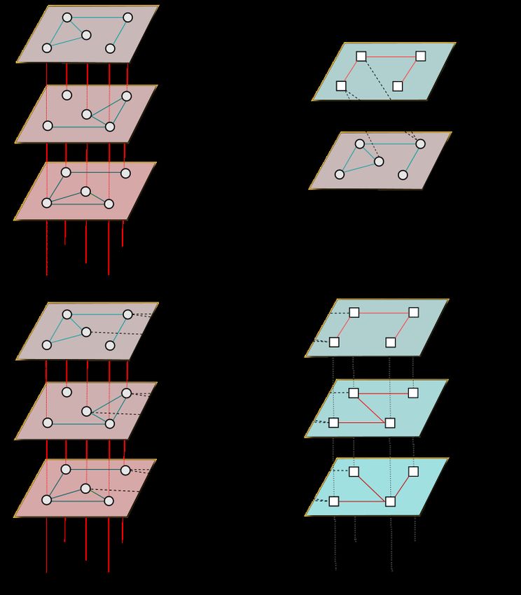
Figure 1: Illustrations of the different types of networks. (A) A multiplex network. The different
layers share the same set of nodes but different types of edges. (B) A heterogeneous network.
The two networks are composed of different types of nodes and edges, connected by bipartite
interactions (black dashed lines). (C) A multiplex-heterogeneous network composed of two
multiplex networks. The multiplex networks are connected by bipartite interactions (dashed lines).
For the sake of simplicity, the figure does not represent all the possible bipartite interactions
(each layer of a given multiplex is in reality linked with every layer of the other multiplex).

                                                3
2 Related work in network embedding
Network embedding relies on two key components: a similarity measure between pairs of nodes
in the original network and a learning algorithm. Given a network and a similarity measure, the
aim of network embedding is to learn a vector representation of the nodes in a lower dimension
space, while preserving as much as possible the similarity. In the next sections we will present
the state-of-the-art of monoplex, multiplex and multiplex-heterogeneous network embedding.
2.1 Monoplex network embedding
Many network embedding methods have been recently developed to study a large variety of
networks, from biological to social ones. The classical method deepwalk [69] inspired a series of
methods such as node2vec [35] and LINE (for Large-scale Information Network Embedding) [83].
Deepwalk uses truncated random walks to compute the node similarity in the network. Then, a
combination of the skip-gram learning algorithm [60] and hierarchical softmax [62] is used to learn
the graph representations. Skip-gram is a model based on natural language processing. It intends
to maximize the probability of co-occurrence of nodes within a walk, focusing on a window, i.e. a
section of the path around the node. Node2vec [35] upgrades deepwalk by introducing negative
sampling during the learning phase [61]. Moreover, node2vec allows biasing the random walks
towards depth or breadth-first random walks, in order to tune the exploration of the search
space. LINE [83] follows a different approach to optimize the embedding: it computes the node
similarity using an adjacency-based proximity measure in association with negative sampling.
Some embedding methods are based on matrix-factorization, such as GraRep [9] or HOPE [68],
and others on deep neural networks such as graph convolutional networks (GCN) [45].
These embedding methods have been applied to link prediction or node labelling tasks. Their
performance rely upon multiple criteria such as the size of the network, its density, the embedding
dimension or the evaluation metrics [33]. Overall, they have been designed to handle monoplex
networks. However, we now have access to a richer representation of complex systems as multiplex
networks, and some recent methods have explored the embedding of such multiplex networks.
2.2 Multiplex network embedding
The most straightforward approach to deal with multiplex networks is to merge the different layers
into a monoplex network [6]. However, this merging creates a new network with its own topology,
and loses the topological features of the individual layers. This new topology is logically biased
towards the initial topology of the denser layers [17]. Different network embedding methods have
been introduced in order to avoid merging multiplex network layers and take advantage of the
multiplex structure [95, 100, 4, 92]. Overall, these approaches are based on truncated random
walks to compute the similarity in the multiplex network. Ohmnet [100] relies on node2vec
[35] and requires the definition of a hierarchy of layers to model dependencies between them.
But usually, this layer hierarchy information is not known or easy to establish, particularly
for multiplex networks such as social or molecular networks. The Scalable Multiplex Network
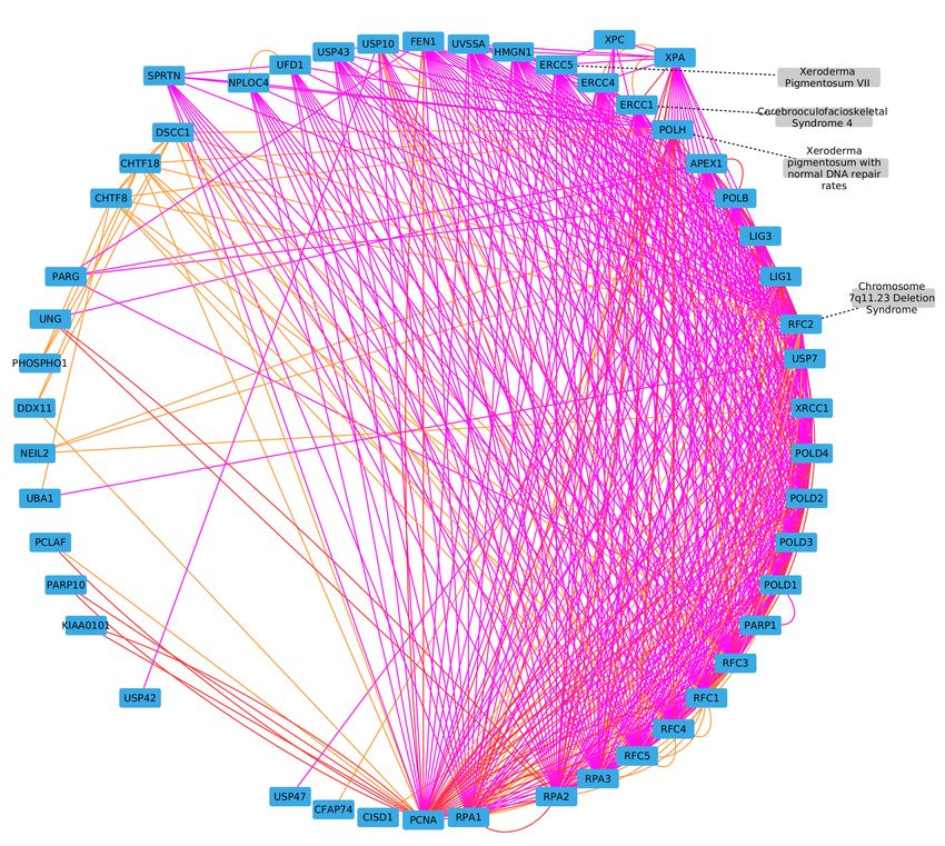
Embedding (MNE) method [95] is also based on node2vec [35]. For each network node, it extracts
one high-dimensional common embedding shared across all the layers of the multiplex network.
In addition, MNE computes a lower-dimensional embedding for every node in each layer of the
multiplex network. Multi-node2vec [92] is another method based on node2vec that constructs the
multiplex embedding with the random walks jumping from one layer to another. Multi-Net [4]
also proposes a random walks procedure in the multiplex network, inspired from [36]. Similarly
to multi-node2vec, the random walks can jump from one layer to another. Multi-Net learns the
embeddings using stochastic gradient descent. The performances of Ohmnet [100], Multi-net [4]
and MNE [95] have been compared in the context of network reconstruction [4]. In this task, the
aim is to reconstruct one layer of the multiplex network from the embeddings of the other layers.
The results show better performances for Multi-net on a set of social and biological multiplex
networks [4].
4Figure 2: Overview of the MultiVERSE pipeline. Starting from a multiplex-heterogeneous
network, we represent its structure through an adjacency matrix (size |V | × |V |); we then compute
a similarity matrix using Random Walk with Restart algorithm, and apply an optimized version
of the VERSE algorithm to compute the embeddings. The resulting matrix of embeddings will
be used for the applications.
2.3 Multiplex-heterogeneous network embedding
Some methods can perform the embedding of heterogeneous networks [24, 77]. A famous approach
is metapath2vec [24]. It extends skip-gram to learn node embeddings for heterogeneous networks
using meta-paths, which are predefined composite relations between different types of nodes.
For instance, in the context of a drug-protein target heterogeneous network, the meta-path
drug-protein target-drug in the network could bias the random walks to extract the information
related to drug combinations.
Nevertheless, to our knowledge, no approach is specifically dedicated to the embedding
of different types of nodes from multiplex-heterogeneous networks. In the next section, we
present formally MultiVERSE, a new method for multiplex and multiplex-heterogeneous network
embedding relying on VERSE [85] and coupled with Random Walks with Restart extended to
Multiplex (RWR-M) and Multiplex-Heterogeneous graphs (RWR-MH) [87].
3 MultiVERSE
In this section, we present the key components of MultiVERSE: the VERSE general framework,
the learning objective, and our particular implementation with Random Walk with Restart for
Multiplex networks (RWR-M) and Random Walk with Restart for Multiplex-Heterogeneous
networks (RWR-MH) (Figure 2). We finally describe the MultiVERSE algorithm.
3.1 VERSE: a general framework for network embedding
The aim of VERSE network embedding is to learn a low-dimensional nonlinear representation
wi of the nodes vi to a d-dimensional continuous vector, where d < n, using Kullback-Leibler
optimization [85]. We denote d the dimension of the embedding space, and n the dimension of the
adjacency matrix. VERSE was originally developed for the embedding of monoplex networks [85].
5The VERSE framework is nevertheless general and versatile enough to be expanded to multiplex
and multiplex-heterogeneous networks.
3.1.1 Similarity distributions
Consider an undirected graph G = (V, E) with V = {vi , i = 1, . . . , n} the set of nodes (|V | = n),
and E ⊆ V × V the set of edges, and simG : V × V → R a given similarity measure on G such
that X
∀v ∈ V, simG (v, u) = 1 . (1)
u∈V
Hence, the similarity for any node v is expressed as a probability distribution simG (v, .). We
note wi the vector representation of node i in the embedding space (W is a (n × d)-matrix).
The (non-normalized) distance or similarity between two nodes embeddings wu and wv is
defined as the dot product wu · wvT . Using the softmax function, we obtain the normalized
similarity distribution in the embedding or vector space:
exp(wv · wT )
simEmb (v, .) = Pn . (2)
i=1 exp(wv · wi )
Finally, the output of any network embedding method is a matrix of embeddings W such as,
∀v ∈ V , simEmb (v, .) ≈ simG (v, .). This requires a learning phase, which is described in the next
section.
3.1.2 Learning objective
This step updates the embeddings at each iteration in order to project simG into the embedding
space leading to the preservation of the topological structure of the graph. In the framework of
VERSE, as simEmb and simG are both probability distributions, this optimization phase aims to
minimize the Kullback-Leibler divergence (KL-divergence) between these two similarities:
X
KL(simG (v, .) k simEmb (v, .)) (3)
v∈VM
We can keep only the parts related to simEmb as it is the target to optimize and simG is
constant. This leads to the following objective function:
X
L=− simG (v, .) log(simEmb (v, .)) (4)
v∈VM
simEmb is defined as a softmax function and needs to be normalized over all the nodes of
the graph at each iteration, which is computationally heavy. Therefore, following the VERSE
algorithm [85], we used Noise Contrastive Estimation (NCE) to compute this objective function
[37, 63]. NCE trains a binary classifier to distinguish node samples coming from the distribution
of similarity in the graph simG and those generated by a noise distribution Q. We define D as
the random variable representing the classes, D = 0 for a node if it has been drawn from the
noise distribution Q or D = 1 if it has been drawn from the empirical distribution and E is the
expected value. With u a node drawn from P and v drawn from simG (u, .), with NCE we draw
s < n negative samples vneg from Q(u).
In this framework, the objective function becomes the negative log-likelihood that we want to
minimize via logistic regression:
X h
LN CE = logPW (D = 1 | simEmb (u, v))
u∼P
v∼simG (u,.) (5)
i
+ s.Evneg ∼Q(u) logPW (D = 0 | simEmb (u, ve))
6where PW is computed as the sigmoid (σ(x) = (1 + e−x )−1 ) of the dot product of the
embeddings wu and wv , and simEmb (u, .) is computed without normalization. It has been proven
that the derivative of NCE converges to gradient of cross-entropy when s increases, but in practice
small values work well [63]. Therefore, we are minimizing the KL-divergence from simG .
Overall, VERSE is a general framework for network embedding with the only constraint
that simG must be defined as a probability distribution. In this work, we computed simG
using Random Walks with Restart on Multiplex (RWR-M) and Random Walks with Restart on
Multiplex-Heterogeneous (RWR-MH) networks [87]. We describe this particular implementation
in the next section.
3.2 Random Walk with Restart on Multiplex and Multiplex-Heterogeneous
networks
3.2.1 Random Walk (RW) and Random Walk with Restart (RWR)
Let us consider a finite graph, G = (V, E), with adjacency matrix A. In a classical RW, an
imaginary particle starts from a given initial node, v0 . Then, the particle moves to a randomly
selected neighbour of v0 with a probability defined by its degree. We can define pt (v) as the
probability for the random walk to be at node v at time t. Therefore, the evolution of the
probability distribution, pt = (pt (v))v∈V , can be described as follows:
pTt+1 = M pTt (6)
where M denotes a transition matrix that is the column normalization of A. The stationary
distribution of Equation (6) represents the probability for the particle to be located at a specific
node for an infinite amount of time [54].
Random Walk with Restart (RWR) additionally allows the particle to jump back to the initial
node(s), known as seed(s), with a probability r ∈ (0, 1) at each step. In this case, the stationary
distribution can be interpreted as a measure of the proximity between the seed(s) and all the
other nodes in the graph. We can formally define RWR by including the restart probability in
Equation (6):
pTt+1 = (1 − r)M pTt + rpT0 (7)
The vector p0 is the initial probability distribution. Therefore, in p0 , only the seed(s) have values
different from zero. Equation (7) can be solved in a iterative way [87].
In our previous work, we expanded the Random Walk with Restart algorithm to Multiplex
(RWR-M) and Multiplex-Heterogeneous networks (RWR-MH) [87]. Below, we show how the
output of RWR-M and RWR-MH can easily be adapted to produce simG , the required input for
the VERSE framework.
3.2.2 Random Walk with Restart on Multiplex networks (RWR-M)
We define a multiplex graph as a set of L undirected graphs, termed layers, which share the
same set of n nodes [46, 21]. The different layers, α = 1, . . . , L, are defined by their respective
n × n adjacency matrices, A[α] = (A[α] (i, j))i,j=1,...,n . A[α] (i, j) = 1 if node i and node j are
connected on layer α, and 0 otherwise [5]. We do not take into account potential self-interactions
and therefore set A[α] (i, i) = 0 ∀ i = 1, . . . , n. In addition, we consider that viα represents the
node i in layer α.
Thus, we can represent a multiplex graph by its adjacency matrix:
A = A[1] , . . . , A[L] (8)
and define it as GM = (VM , EM ), where:
VM = {viα , i = 1, . . . , n, α = 1, . . . , L} ,
n o[
EM = (viα , vjα ), i, j = 1, . . . , n, α = 1, . . . , L, A[α] (i, j) 6= 0
n o
(viα , viβ ), i = 1, . . . , n, α 6= β .
7RWR-M should ideally explore in parallel all the layers of a multiplex graph to capture as
much topological information as possible. Therefore, a particle located in a given node, viα , may
be able to either walk to any of its neighbours within the layer α or to jump to its counterpart
node in another layer, viβ with β 6= α [20]. Additionally, the particle can restart in the seed
node(s) on any layer of the multiplex graph. In order to match these requirements, we previously
defined a multiplex transition matrix and expanded the restart probability vector, allowing us to
apply Equation (6) on multiplex graphs [87].
In this study, we independently run the RWR-M algorithm n times, using each time a different
node as seed. This allows measuring the distance from every single node to all the other nodes in
the multiplex graph. This node-to-node distance matrix is actually
P a probability distribution
describing the particle position in the steady state, where u∈VM simG (v, u) = 1 ∀ v ∈ VM ,
therefore fulfilling the requirements of the VERSE input. We set the RWR-M parameters to the
same values used in our original study (r = 0.7, τ = (1/L, 1/L, . . . , 1/L), δ = 0.5) [87].
3.2.3 Random Walk with Restart on Multiplex-Heterogeneous networks (RWR-
MH)
A heterogeneous graph is composed of two graphs with different types of nodes and edges. In
addition, it also contains a bipartite graph in order to link the nodes of different type (bipartite
edges) [49]. In our previous study [87], we described how to extend the RWR to a graph which is
both multiplex and heterogeneous. However, this study considered only one multiplex graph in
the multiplex-heterogeneous graph. For the present work, we additionally expanded RWR-MH to
a complete multiplex-heterogeneous graph, i.e. both components of the heterogeneous graph can
be multiplex (Figure 1, C), based on the work of [26]. Let us consider a L-layers multiplex graph,
GM = (VM , EM ), with n × L nodes, VM = {viα , i = 1, . . . , n, α = 1, . . . , L}. We also define a
second L-layers multiplex graph, with m × L nodes, UM = uα j , j = 1, . . . , m, α = 1, . . . , L .
We additionally need a bipartite graph GB = (VM ∪ UM , EB ) with EB ⊆ VM × UM . The edges
of the bipartite graph only connect pairs of nodes from the different sets of nodes, VM and
UM . It is to note that the bipartite edges should link nodes with every layer of the multiplex
[α] [α]
graphs. We therefore need L identical bipartite graphs, GB = (VM ∪ UM , EB ) to define
the multiplex-heterogeneous graph. We can then describe a multiplex-heterogeneous graph,
GM H = (VM H , EM H ), as:
VM H = {VM ∪ UM }
n o
[α]
EM H = ∪α=1,...,L EB ∪ EVM ∪ EUM
In the RWR-MH algorithm, the particle should be allowed to move in any of the multiplex
graphs as described in the RWR-M section. In addition, it may be able to jump from a node in
one multiplex graph to the other multiplex graph following a bipartite edge. We also have to
bear in mind that the particle could now restart in different types of node(s), i.e. we can have
seed(s) of different category (see Figure 1, C). We accordingly defined a multiplex-heterogeneous
transition matrix and expanded the restart probability vector. This gave us the opportunity to
extent and apply Equation (6) on multiplex-heterogeneous graphs [87, 26].
In the context of MultiVERSE, we independently run the RWR-MH algorithm n + m times.
In each execution, we select a different seed node until all the nodes from both multiplex graphs
have been used as individual seeds. P As a result, we can define a node-to-node distance matrix
matching VERSE input criteria, i.e u∈VM H simG (v, u) = 1 ∀ v ∈ VEM . We set the RWR-MH
parameters to the same values used in the original study (r = 0.7, τ = (1/L, 1/L, . . . , 1/L),
δ = 0.5, λ = 0.5, η = 0.5) [87].
3.3 MultiVERSE algorithm
Algorithm 1 presents the pseudo-code of MultiVERSE based on RWR on multiplex and multiplex-
heterogeneous networks [87] and Kullback-Leibler optimization from the VERSE algorithm
[85].
8Our implementation of VERSE with NCE is slightly different from the original. We perform
first the RWR-M or RWR-MH for all the nodes of the network in order to obtain the similarity
distribution simGM . The output of this step is the probability matrix p, where pu is the
probability vector representing the similarities between u and all the other nodes. The matrix of
the embedded representation of the nodes, W , is randomly initialized. For each iteration, from
one node u sampled randomly from a uniform distribution U, we filter the probability vector pu .
We keep the Nmax highest probabilities because the shape of the distribution of probabilities
falls very fast to very low probabilities. Doing so, we can speed up the calculation by filtering
out the lowest probabilities and by reducing the size of the similarity matrix. We normalize this
resulting probability vector ṗu , and sample one node v according to its probability in pu . We set
empirically the parameter Nmax = 300 for large networks (number of nodes exceeding 5000). For
smaller networks, we set this parameter to 10% − 20% of the number of nodes of the network,
depending on the shape of the distribution. These two steps (lines 6 and 7) were not in the
original VERSE. We parallelized the repeat loop (line 4) and added a parallelized for loop after
line 5 in order to run the code from line 6 to 12 in parallel P times. In our simulations, we set
P = 100.
Algorithm 1 MultiVERSE algorithm
1: Input: a multiplex graph, Nmax , s
2: W ← N (0, 1)
3: p ← RWR-M(H)(GM )
4: repeat
5: u∼U
6: ṗu = Normalize(pu (1, ..., Nmax ))
7: vpos ∼ ṗu
8: Wu , Wvpos ← U pdate(u, vpos , 1, biaspos )
9: for i=1, ... , s do
10: vneg ∼ Q(u)
11: Wu , Wvneg ← U pdate(u, vneg , 0, biasneg )
12: end for
13: until Maximum step reached
Then, we update Wu and Wv according to algorithm 2 by reducing their distances in the
embedding space. We added the bias for NCE: biaspos = log(N ) and biasneg = log(N/s).
Algorithm 2 Update
1: Input: u, v, D, bias, lr
2: g ← [D − σ(Wu · Wv − bias)] ∗ lr
3: Wu ← g · Wv
Then, s negative nodes are sampled from Q(u) and we update the corresponding embeddings
by increasing their distances in the embedding space. The update can also be seen as the training
part with lr as the learning rate of the binary classifier of the NCE estimation as described in
equation 5. The whole process is repeated until the maximum steps are reached.
MultiVERSE is freely available on github at https://github.com/Lpiol/MultiVERSE.
4 Evaluation protocol
We propose a benchmark to compare the performance of MultiVERSE and other embedding
methods for multiplex and multiplex-heterogeneous networks. The performances are evaluated
through link prediction for both multiplex and multiplex-heterogeneous networks, and with
network reconstruction for multiplex networks.
94.1 Evaluation of multiplex network embedding
In the next sections, we describe the datasets, the evaluation tasks and the methods used for
evaluations.
4.1.1 Multiplex network datasets
We used 7 multiplex networks (2 molecular, 1 disease, 1 neuronal, 1 co-authorship and 2 social
networks) to evaluate the different approaches of multiplex network embedding. The networks
CKM, LAZEGA, C.ELE, ARXIV, and HOMO have been extracted from the CoMuNe lab
database https://comunelab.fbk.eu/data.php. We constructed the other two networks, DIS
and MOL. A description of each of these multiplex networks follows. The number of nodes and
edges of the different layers are detailed in Table 1.
• CKM physician innovation (CKM) is a multiplex network describing how physicians
in four towns in Illinois used the new drug tetracycline [13]. It is composed of 3 layers
corresponding to three questions asked to the physicians: i) to whom do you usually turn
when you need information or advice about questions of therapy? ii) who are the three or
four physicians with whom you most often find yourself discussing cases or therapy in the
course of an ordinary week – last week for instance? iii) would you tell me the first names
of your three friends whom you see most often socially?
• Lazega network (LAZEGA) is a multiplex social network composed of 3 layers based
on co-working, friendship and advice between partners and associates of a corporate law
partnership [28].
• Caenorabidis Elegans connectome (C.ELE) is a neuronal multiplex network composed
of 3 layers corresponding to different synaptic junctions [11, 19]: electrical, chemical poladic
and chemical monadic.
• ArXiv network (ARXIV) is composed of 8 layers corresponding to different ArXiv
categories. The dataset has been restricted to papers with ’networks’ in the title or abstract,
up to May 2014 [18]. The original data from the CoMuNe Lab database is divided in 13
layers. We extracted the 8 layers (1-2-3-5-6-8-11-12) containing more than 1000 edges.
• Homo sapiens network (HOMO) is composed of 4 layers extracted from the original
network on CoMuNe Lab [19], keeping physical association, direct interaction, association
and co-localization layers. The data are initially extracted from BioGRID [81]
• Disease multiplex network (DIS) has been constructed, composed of 3 layers: i) A
disease-disease network based on a projection of a disease-drug network from the Compara-
tive Toxicogenomics Database (CTD) [15] extracted from BioSNAP [101]. In this network,
an edge between two diseases is created if the Jaccard Index between the neighborhoods of
the two nodes in the original bipartite network is superior to 0.4. Two diseases are thereby
linked if they share a similar set of drugs. This projection has been done using NetworkX [38].
ii) A disease-disease network where the edges are based on shared symptoms. The network
has been constructed from the bipartite disease-symptoms network from [99]. Similarly to
[99], we use the cosine distance to compute the symptom-based diseases similarity for this
network. We kept for the disease-disease network all interactions with a cosine distance
superior to 0.5 iii) A comorbidity network from epidemiological data extracted from [43].
• Human molecular multiplex network (MOL) is a molecular network, consisting
of 3 layers: i) A protein-protein interaction (PPI) layer corresponding to the fusion of
3 datasets: APID (apid.dep.usal.es) (Level 2, human only), Hi-Union and Lit-BM
(http://www.interactome-atlas.org/download). ii) A pathways layer extracted from
NDEx [71] and corresponding to the human Reactome data [14]. iii) A molecular complexes
layer constructed from the fusion of Hu.map [25] and Corum [31], using OmniPathR [86].
10Dataset Layers Nodes Edges
1 215 449
CKM 2 231 498
3 228 423
1 71 717
LAZEGA 2 69 399
3 71 726
1 253 514
C.ELE 2 260 888
3 278 1703
1 1558 3013
2 5058 14387
3 2826 6074
4 1572 4423
ARXIV
5 3328 7308
6 1866 4420
7 1246 1947
8 4614 11517
1 12345 48528
2 14770 83414
HOMO
3 1626 1953
4 5680 18381
1 3891 117527
DIS 2 4155 101104
3 434 3137
1 14704 122211
MOL 2 7926 194500
3 8537 63561
Table 1: Description of the 7 multiplex networks used for the evaluation protocol.
4.1.2 Methods implemented for comparisons
We compare MultiVERSE with 6 methods designed for monoplex network embedding (deepwalk,
node2vec, LINE) and multiplex network embedding (Ohmnet, MNE, Multi-node2vec), and 4 link
prediction heuristic scores (only in the link prediction task).
Monoplex network embedding methods
• deepwalk [69]: This method is based on non-biased random walks, and apply the skip-gram
algorithm [60] to learn the embeddings. We set the context window to 10, and the number
of random walks to start at each node to 10.
• node2vec [35]: This method is an extension of deepwalk with a pair of parameters p and q
that biases the random walks for Breadth-first Sampling or Depth-first Sampling. We set
p = 2 and q = 1 to promote moderate explorations of the random walks from a node, as
stated in [35]. We set the other parameters as for deepwalk.
• LINE [83]: LINE is not based on random walks, but computes the similarities using an
adjacency-based proximity measure in association with negative sampling. It approximates
the first and second order proximities in the network from one node. First order proximity
refers to the local pairwise proximity between the nodes in the network (only neighbours),
and second order proximity look for nodes sharing many connections. We set the negative
ratio to 5.
11Score Definition
|N (u)∩N (v)|
Jaccard Coefficient (JC) |N (u)∪N (v)|
Common neighbours (CN) |N (u) ∩ N (v)|
1
P
Adamic Adar (AA) t∈|N (u)∩N (v)| log |N (t)|
Preferential attachment (PA) |N (u)|.|N (v)|
Table 2: Definition of the heuristic scores of a link (u, v) in the graph G(V, E). N (u) denotes the
set of neighbour nodes of node u ∈ V in G(V, E).
Multiplex network embedding methods
• OhmNet [100]: This approach takes into account the multi-layer structure of multiplex
networks. It is a random walk-based method that uses node2vec to learn the embeddings
layer by layer. We applied the same parameters as in node2vec. The user has to define a
hierarchy between layers. We created a 2-level hierarchy for all multiplex networks with
first layer as the higher in the hierarchy and the other layers are defined at the second level
of the hierarchy, in the same way as [4].
• MNE [95]: This method is also designed for multiplex networks and uses node2vec to
learn the embeddings layer by layer. For each node, MNE computes a high-dimensional
common embedding and a lower-dimensional additional embedding for each type of relation
of the multiplex network. The final embedding is computed using a weighted sum of these
two high-dimensional and low-dimensional embeddings. We used the default parameters
(https://github.com/HKUST-KnowComp/MNE).
• Multi-node2vec [92]: This multiplex network embedding method is also based on node2vec.
The random walks can jump to different layers and explore in this way the multiplex
neighborhood. The length of the random walks is set to 100.
We used OpenNE (https://github.com/thunlp/OpenNE) to implement deepwalk, node2vec
and LINE. The other methods have been implemented from the source code associated to the
different publications.
Link prediction heuristics
In order to evaluate the relevance of the aforementioned network embedding methods, we also
compared them with four classical and straightforward link prediction heuristic scores for node
pairs [35]. Table 2 provides formal definitions of these heuristic scores.
4.1.3 Evaluation tasks
On multiplex networks, we evaluate the different methods by measuring their performances in
two different tasks: link prediction and network reconstruction. For all the evaluations, we set
the embedding dimension to d = 128 as in [35, 100, 69], and used the package EvalNE v0.3.1 [59].
From node embeddings to edges
MultiVERSE and the other embedding methods allow learning vector representations of nodes from
networks. We aim here to test their performance on link prediction and network reconstruction.
We hence need to predict whether an edge exists between every pairs of node embeddings. To do
so, given two nodes u and v, we define an operator ◦ over the corresponding embeddings f (u) and
f (v). This gives g : V × V → Rd , with d the dimension of the embeddings, V the set of nodes and
g(u, v) = f (u) ◦ f (v). Our test network contains both true and false edges (present and absent
12Operators Symbol Definition
fi (u)∗fi (v)
Hadamard [f (u) f (v)]i = 2
Average [f (u) f (v)]i = fi (u) + fi (v)
Weighted-L1 k . k1 k fi (u).fi (v) k1 i =| fi (u) − fi (v) |
Weighted-L2 k . k2 k fi (u).fi (v) k2 i =| fi (u) − fi (v) |2
fi (u)∗fi (v)
Cosine cos cos[f (u), f (v)]i = kfi (u)kkfi (v)k
Table 3: Embedding operators used to predict edges in the tasks of link prediction and network
reconstruction. The definitions describe the ith components of g(u, v).
edges, respectively). We apply five different operators ◦: Hadamard, Average, Weighted-L1,
Weighted-L2 and Cosine (Table 3)).
The outputs of the embedding operators are used to feed a binary classifier for the evaluation
tasks. This classifier aims to predict if there is an edge or not between two nodes embeddings.
Similarly, we use the output of the four link prediction heuristic scores described in Table 2 with
a binary classifier to predict edges in a multiplex network.
Link prediction
We first evaluate the performance of the different methods to predict links removed from the
original multiplex networks (Figure 3). We remove 30% of the links in each layer of the original
networks. We applied the Andrei Broder algorithm [7] in order to randomly select the links to be
removed while keeping a connected graph in each layer. This step provides the multiplex training
network, to which we apply the 3 categories of methods (see Figure 3):
• The methods specifically designed for monoplex network embedding (node2vec, deepwalk
and LINE) are applied individually on each layer of the multiplex networks. We thereby
obtain one embedding per layer and average them (arithmetic mean) in order to obtain a
single embedding for each node. We then apply the embedding operators. We refer to these
approaches in the results section as node2vec-av, deepwalk-av and LINE-av.
• Methods specifically designed for multiplex network embedding (Ohmnet, MNE, Multi-
node2vec) are applied directly on the training multiplex network. We then apply the
embedding operators.
• The link prediction heuristic scores JC, CN, AA and PA are applied individually on each
layer of the multiplex networks. We then average the scores, as JC-av, CN-av, AA-av, and
PA-av.
From the outputs of the embedding operators and heuristic scores, we feed and train a binary
classifier and then test it on the 30% of test edges that have been removed initially. The binary
classifier is a logistic regressor.
The evaluation metrics for link prediction is ROC-AUC as it is commonly used for embedding
evaluation on link prediction and to validate network embedding [95, 35]. The ROC-AUC is
computed as the area under the ROC curve, which plots the true positive rate (TPR) against the
false positive rate (FPR) at various threshold settings. An AUC value of 1 represent a model
that classifies perfectly the samples.
Network reconstruction
Network reconstruction is another approach to evaluate network embedding methods [91, 4, 32].
In this case, the goal is to quantify the amount of topological information captured by the
embedding methods. This is equivalent to predict if we can go back from the embedding to the
original adjacency matrix of each layer of the multiplex network.
13Figure 3: General approach for link prediction on multiplex networks: (top) for the link prediction
heuristics, we apply them to each layer and average them across all layers ; (center) for monoplex-
based methods, we embed each layer with the given method, then average it ; (bottom) for
multiplex-based methods, we apply the specific embedding method to the network. The embedding
operators are then applied to monoplex- and multiplex-based method embeddings. The three
types of methods are finally evaluated for link prediction using a binary classifier and a ROC-AUC
is computed.
Theoretically, to reconstruct the networks, one would need to apply link prediction to every
possible edge in the graphs. This is however in practice not scalable to large graphs. Indeed, it
would correspond to n(n − 1)/2 potential edges to classify (for undirected networks of n nodes
without self-loops). In addition, the networks in our study are sparse, with much more false
(absent) than true (present) edges, leading to large class imbalance. In this context, ROC-AUC
can be misleading, as large changes in the ROC Curve or ROC-AUC score can be caused by a
small number of correct or incorrect predictions [29]. In order to account for class imbalance, we
used the precision@K [91]. This evaluation metric is based on the sorting in descending order of
all predictions and consider the first K best predictions to evaluate how many true edges (the
minority class) are predicted correctly by the binary classifier. From the outputs of the embedding
operators, we perform network reconstruction by training a binary classifier on a subset of the
original networks (Figure 4). We choose a subset of 95% of the edge pairs from the original
adjacency matrix of each layer for the smaller multiplex networks (CKM, LAZEGA and C.ELE)
to construct the training graph. As the class imbalance increases with the number of nodes and
sparsity of the networks, we choose smaller subsets for the largest networks, respectively 5%
of edges for the ARXIV network and 2.5% for the other networks, as in previous publications
[32, 91]. For each layer, K is defined as the maximum of true edges in this subset of edge pairs.
We use a Random Forest algorithm as a binary classifier for network reconstruction, as it is known
to be less sensitive to class imbalance [65]. In network reconstruction, the results correspond to
the training phase of the classifier, there is no test phase.
4.2 Evaluation of multiplex-heterogeneous network embedding
4.2.1 Multiplex-heterogeneous network datasets
• Gene-disease multiplex-heterogeneous network: We use the two multiplex networks
presented in the previous sections: the disease (DIS) and molecular multiplex networks
(MOL) (Table 1). In addition, we extracted the curated gene-disease bipartite network from
the DisGeNET database [70] in order to connect the two multiplex networks. This bipartite
interaction network contains 75445 interactions between 5188 diseases and 9179 genes. We
14Figure 4: General approach for network reconstruction on multiplex networks: (top) for monoplex-
based methods, embed each layer with the given method, then average it ; (bottom) for multiplex-
based methods, apply the specific embedding method to the network. Embedding operators are
then applied to monoplex- and multiplex-based method embeddings. The three types of methods
are finally evalutated for network embedding using a binary classifier and a precision@K score is
computed.
obtain a multiplex-heterogeneous network, as represented in Figure 1C.
• Drug-target multiplex-heterogeneous network: We use the molecular multiplex net-
work (MOL) from the previous multiplex-heterogeneous network. We constructed the follow-
ing 3-layers drug multiplex network: (i) the first layer (2795 edges, 877 nodes) has been ex-
tracted from Bionetdata (https://rdrr.io/cran/bionetdata/man/DD.chem.data.html)
and the edges correspond to Tanimoto chemical similarities between drugs if superior to
0.6, (ii) the second layer (678 edges, 362 nodes) comes from [12] and the edges are based on
drug combinations as reported in clinical data, (iii) the third layer (13397 edges, 658 nodes)
is the adverse drug–drug interactions network available in [12]. The drug-target bipartite
network has been extracted from the same publication [12], and contains 15030 bipartite
interactions between 4412 drugs and 2255 protein targets.
4.2.2 Evaluation task
We validate the multiplex-heterogeneous network embedding using link prediction. We remove
randomly 30% of the edges but only from the bipartite interactions to obtain a training graph.
We then train a Random Forest on the training graph, and test on the 30% removed edges. Based
on the multiplex-heterogeneous networks described previously, the idea behind this evaluation is
to test if we can predict gene-disease and drug-gene links. Comparisons with other approaches
are not possible as, to our knowledge, no existing multiplex-heterogeneous network embedding
method are currently available in the literature.
4.3 Case study: discovery of new gene-disease associations
Link prediction
Our aim for this case-study is to predict new gene-disease links. We thereby applied MultiVERSE
on the full gene-disease multiplex-heterogeneous network without removing any edges, and trained
a binary classifier (Random Forest) using edges from the bipartite interactions. Then, we test all
possible gene-disease edges that are not in the original bipartite interactions and involve Progeria
and Xeroderma pigmentosum VII disease nodes. Finally, we select the top 5 new gene-disease
associations for each disease.
15Clustering
We also applied MultiVERSE to the gene-disease multiplex-heterogeneous gene-disease network,
followed by spherical K-means [8] to cluster the vector representations of nodes. Spherical
K-means clustering is well-adapted to high-dimensional clustering [97]. We define the number of
clusters for spherical K-means to 500, in order to obtain cluster sizes that can be analysed from a
biological point of view.
5 Results
5.1 Evaluation results for multiplex network embeddings
5.1.1 Link prediction
We evaluate the performance of the different methods (link prediction heuristics and network
embedding) on the task of link prediction applied to the set of multiplex networks. First, we
can observe that the heuristics are not efficient for link prediction, with ROC-AUC only slightly
better than random classification (Table 4).
The methods based on embedding always perform better than the heuristic baselines. In
addition, the ROC-AUC is in most of the cases higher when the models take into account
the multiplex network structure rather than the monoplex-average, as observed in [95]. For
instance, using the Hadamard operator, the ROC-AUC average over all the networks of the
three monoplex-average approaches (node2vec-av, deepwalk-av, LINE-av) is 0.8025, whereas the
average of the three multiplex-based approaches (Ohmnet, MNE, Multi-node2vec) is 0.8381. The
ROC-AUC score average of MultiVERSE in this context is 0.9011. Nevertheless, node2vec-av
and deepwalk-av perform very well and even outperform multiplex-based approaches on various
scenarios, for instance link prediction on the C.ELE and ARXIV networks.
MultiVERSE combined with the Hadamard operator outperforms the other methods for all
the tested networks but CKM. In addition, MultiVERSE is the best approach when combined
with three out of five operators (Hadamard, Average, Cosine). These results suggest that RWR-M
is able to better capture the topological features of the networks under study.
5.1.2 Network reconstruction
We next evaluate the performances of the different embedding methods on the task of network
reconstruction applied to multiplex networks. As described in section 4.1.3, we now rely on the
evaluation metric, precision@K. The experimental results are shown in Table 5.
On one hand, for the small networks (i.e., CKM, LAZEGA and C.ELE), the best precision
is achieved with LINE-av in combination with any of the operators but Cosine. In particular,
LINE-av obtains a perfect score for the CKM network using the Weighted-L2 or Hadamard
operators. MNE is in second position with more than 99% of precision using the Weighted-L1 or
Weighted-L2 operators. LINE-av also presents good performances for the C.ELE network with a
precision of 93.67% using the Weighted-L2 operator, almost 20% higher than the second best
method on this network (Multi-node2vec with a score of 0.7568 using the Weighted-L2 operator).
On the other hand, we can group together the results obtained for the large networks
(DIS, ARXIV, HOMO and MOL). In this case, MultiVERSE achieves the best performance in
combination with different operators. Large networks are sparse, leading to high class imbalance
(4.1.3). Still, MultiVERSE achieves a good score for the HOMO and DIS networks, with
precision@K of 0.8729 and 0.6784, respectively. The precision obtained on the molecular network
(MOL) is the lowest, with a precision@K of 0.4143. The complexity of the task is possibly higher
as the number of nodes and class imbalance increase.
Overall, the lowest scores are obtained by MNE and, in general, the Cosine operator performs
poorly for all methods. The network reconstruction process is a complex task, and the perfor-
mance depends on the size and density of the different layers composing the multiplex network.
Nevertheless, MultiVERSE obtains good results for most of the networks without any processing
of the imbalanced data.
16Operators Method CKM LAZEGA C.ELE ARXIV DIS HOMO MOL
CN-av 0.4944 0.6122 0.5548 0.5089 0.5097 0.5113 0.5408
AA-av 0.4972 0.6105 0.549 0.5081 0.5428 0.5112 0.5404
Link prediction heuristics
JC-av 0.4911 0.523 0.5424 0.5113 0.5425 0.5113 0.5433
PA-av 0.5474 0.6794 0.5634 0.5139 0.496 0.5185 0.5278
node2vec-av 0.7908 0.6372 0.8552 0.9775 0.9093 0.8638 0.8753
deepwalk-av 0.7467 0.6301 0.8574 0.9776 0.9107 0.8638 0.8763
LINE-av 0.5073 0.4986 0.5447 0.8525 0.9013 0.8852 0.8918
Hadamard
Ohmnet 0.7465 0.7981 0.833 0.9605 0.9333 0.9055 0.8613
MNE 0.5756 0.6356 0.794 0.9439 0.9099 0.8313 0.8736
Multi-node2vec 0.8182 0.7884 0.8375 0.9581 0.8528 0.8592 0.8835
MultiVERSE 0.8177 0.8269 0.8866 0.9937 0.9401 0.917 0.9259
node2vec-av 0.7532 0.737 0.8673 0.9738 0.885 0.6984 0.7976
deepwalk-av 0.7226 0.7094 0.8635 0.9751 0.8888 0.7142 0.8089
LINE-av 0.6091 0.5776 0.6192 0.7539 0.8586 0.7439 0.7792
Weighted-L1
Ohmnet 0.7421 0.7849 0.8128 0.8488 0.8503 0.7007 0.6983
MNE 0.6289 0.6523 0.8019 0.7805 0.8313 0.7619 0.8182
Multi-node2vec 0.8611 0.8089 0.8261 0.9659 0.8628 0.8472 0.8997
MultiVERSE 0.7043 0.7789 0.7516 0.8647 0.7754 0.683 0.7273
node2vec-av 0.7556 0.6851 0.8691 0.9743 0.8867 0.7048 0.8028
deepwalk-av 0.7221 0.6904 0.864 0.9771 0.8891 0.7145 0.813
LINE-av 0.5851 0.5756 0.6275 0.7609 0.8621 0.7429 0.7835
Weighted-L2
Ohmnet 0.7505 0.7788 0.8166 0.8439 0.8599 0.7041 0.6992
MNE 0.601 0.5397 0.7999 0.7815 0.8333 0.7483 0.8122
Multi-node2vec 0.8637 0.8091 0.8282 0.968 0.8675 0.8525 0.9004
MultiVERSE 0.7125 0.7801 0.7441 0.8661 0.7808 0.6918 0.7475
node2vec-av 0.59 0.6596 0.6842 0.6615 0.8256 0.8308 0.777
deepwalk-av 0.5954 0.657 0.6784 0.6582 0.8267 0.8307 0.7737
LINE-av 0.5465 0.6581 0.6699 0.6465 0.8477 0.8653 0.8276
Average
Ohmnet 0.5764 0.656 0.7334 0.6772 0.8533 0.8825 0.7962
MNE 0.5882 0.6615 0.7028 0.6723 0.8242 0.8024 0.783
Multi-node2vec 0.5571 0.6584 0.7365 0.6657 0.8222 0.8216 0.7589
MultiVERSE 0.5963 0.6728 0.7438 0.6752 0.8586 0.8643 0.812
node2vec-av 0.7805 0.7335 0.8515 0.9711 0.8643 0.7368 0.8105
deepwalk-av 0.7465 0.7066 0.8416 0.9724 0.8667 0.7512 0.8079
LINE-av 0.545 0.5126 0.5477 0.8198 0.7409 0.6745 0.816
Cosine
Ohmnet 0.7898 0.7352 0.8094 0.9642 0.859 0.7829 0.7909
MNE 0.6203 0.6506 0.7877 0.8951 0.8347 0.6474 0.8102
Multi-node2vec 0.8532 0.7931 0.7815 0.9435 0.7151 0.8477 0.8884
MultiVERSE 0.8148 0.8171 0.8719 0.9909 0.8775 0.8776 0.9103
Table 4: ROC-AUC scores for link prediction on the 7 reference multiplex networks, for link
prediction heuristics (CN-av, AA-av, JC-av, PA-av) and network embedding methods combined
with different operators (Hadamard, Weighted-L1, Weighted-L2, Average, and Cosine). For each
multiplex network, the best score is in bold; for each operator, the best scores are underlined.
Overall, the MultiVERSE algorithm combined with the Hadamard shows the best scores.
5.2 Evaluation results for multiplex-heterogeneous network embedding
The task of link prediction on multiplex-heterogeneous networks is applied to MultiVERSE
only, as to our knowledge no other methods exist for the embedding of multiple nodes from
multiplex-heterogeneous networks. MultiVERSE has a score of ROC-AUC superior to 0.9 with
the Hadamard and Average operators (Table 6), meaning that the method can predict with high
precision the gene-disease and drug-disease links from the corresponding multiplex-heterogeneous
networks.
17CKM LAZEGA C.ELE ARXIV DIS HOMO MOL
Operators Method
(95%) (95%) (95%) (5%) (2,5%) (2,5%) (2.5%)
node2vec-av 0.6764 0.9174 0.4526 0.8207 0.5578 0.7599 0.2989
deepwalk-av 0.6564 0.9351 0.4416 0.7886 0.5486 0.7636 0.3164
LINE-av 1.0 0.9924 0.8924 0.8204 0.4955 0.5191 0.4006
Hadamard
Ohmnet 0.7842 0.8334 0.5329 0.9156 0.4811 0.6979 0.2591
MNE 0.9505 0.9094 0.2728 0.7891 0.4218 0.3641 0.1316
Multi-node2vec 0.8352 0.8811 0.6875 0.8605 0.6063 0.7584 0.3123
MultiVERSE 0.9687 0.9695 0.7436 0.9015 0.6734 0.8729 0.3674
node2vec-av 0.5923 0.9494 0.5129 0.6922 0.5859 0.8123 0.3194
deepwalk-av 0.5791 0.9784 0.4896 0.6878 0.5921 0.7984 0.3206
LINE-av 0.9985 0.9953 0.9229 0.7837 0.4921 0.6839 0.3586
Weighted-L1
Ohmnet 0.7355 0.8581 0.5785 0.8771 0.6025 0.8019 0.3769
MNE 0.9926 0.975 0.4722 0.8593 0.4377 0.5241 0.1861
Multi-node2vec 0.8636 0.9235 0.7379 0.7684 0.6356 0.7649 0.2671
MultiVERSE 0.8545 0.9638 0.7444 0.8705 0.6678 0.7913 0.3559
node2vec-av 0.5886 0.9436 0.5097 0.6983 0.5953 0.8193 0.352
deepwalk-av 0.5829 0.9672 0.5146 0.6877 0.5857 0.805 0.3233
LINE-av 1.0 0.9962 0.9367 0.7749 0.4945 0.6697 0.392
Weighted-L2
Ohmnet 0.7418 0.8687 0.5724 0.8694 0.6209 0.8143 0.3701
MNE 0.9926 0.9764 0.4646 0.8818 0.4351 0.5529 0.176
Multi-node2vec 0.8644 0.93 0.7568 0.7548 0.6361 0.7896 0.2922
MultiVERSE 0.8653 0.969 0.754 0.8776 0.6784 0.7876 0.3701
node2vec-av 0.8408 0.917 0.4817 0.889 0.5587 0.6809 0.2686
deepwalk-av 0.8331 0.9379 0.501 0.8853 0.5318 0.6714 0.2795
LINE-av 0.9855 0.9382 0.7103 0.8725 0.5093 0.5677 0.3244
Average
Ohmnet 0.9412 0.8287 0.5825 0.906 0.4989 0.6551 0.2887
MNE 0.9179 0.9151 0.2966 0.7146 0.4175 0.352 0.1444
Multi-node2vec 0.9767 0.8937 0.6726 0.9498 0.6243 0.6216 0.2901
MultiVERSE 0.978 0.9059 0.5326 0.9758 0.6316 0.7204 0.4143
node2vec-av 0.5103 0.4936 0.18 0.2537 0.1825 0.116 0.0441
deepwalk-av 0.4807 0.4776 0.1741 0.2835 0.1854 0.1036 0.0462
LINE-av 0.3291 0.4974 0.1867 0.2638 0.2384 0.1476 0.0454
Cosine
Ohmnet 0.5696 0.509 0.1718 0.2655 0.1984 0.1311 0.044
MNE 0.3169 0.4536 0.1768 0.2445 0.1957 0.1667 0.044
Multi-node2vec 0.5127 0.52 0.186 0.273 0.195 0.1032 0.0461
MultiVERSE 0.6395 0.5026 0.1818 0.254 0.1983 0.1522 0.0474
Table 5: precision@K scores for network reconstruction on the 7 reference multiplex networks,
for the network embedding methods combined with different embeddings operators (Hadamard,
Weighted-L1, Weighted-L2, Average, and Cosine). For each multiplex network, the best score
is in bold; for each operator, the best score is underlined. The percentage of edges used for
the reconstruction is indicated in parenthesis under the name of the network. In the case of
large networks (DIS, ARXIV, HOMO and MOL) MultiVERSE achieves the best performance in
combination with different operators.
5.3 Case study results: discovery of new gene-disease associations
5.3.1 Discovery of new gene-disease associations with link prediction
The results of the evaluations on multiplex-heterogeneous network link prediction show that
MultiVERSE combined with the Hadamard and Average operators reach ROC-AUC scores
superior to 0.9 (Table 6). We here investigate in detail the top 5 new gene-disease associations
predicted by MultiVERSE combined with these operators for Hutchinson-Gilford Progeria
Syndrome (HGPS) and Xeroderma pigmentosum VII (Table 7) .
18Operators Gene-Disease Bipartite Drug-target Bipartite
Hadamard 0.95 0.9701
Weighted-L1 0.7962 0.8057
Weighted-L2 0.7951 0.8055
Average 0.9603 0.9703
Cosine 0.7765 0.8338
Table 6: ROC-AUC scores for link prediction using MultiVERSE on 2 multiplex-heterogeneous
reference networks. Link predictions are computed for the bipartite interactions of the multiplex-
heterogeneous networks. The scores higher than 0.9 are highlighted in bold.
HGPS Xeroderma p. VII
Average Hadamard Average Hadamard
NOS2 POT1 TNF TNF
IL6 TERF1 SOD2 VCAM1
TNF EEF1A1 IL6 NUP62
SOD1 TERF2 TP53 ERCC2
SOD2 TERF2IP FN1 MCC
Table 7: Top 5 predictions of new gene-disease associations for HGPS and Xeroderma pigmentosum
VII by MultiVERSE combined with Average and Hadamard operators.
Hutchinson-Gilford Progeria Syndrome
Hutchinson-Gilford Progeria Syndrome (HGPS) is a rare premature aging genetic disease character-
ized by postnatal growth retardation, midface hypoplasia, micrognathia, premature atherosclerosis,
coronary artery disease, lipodystrophy, alopecia and generalized osteodysplasia [22]. HGPS is
caused by mutations in the LMNA genes that cause the production of a toxic form of the Lamin
A protein called Progerin.
MultiVERSE top predictions reveal interesting candidate genes (Table 7). In particular,
NOS2 encodes a nitric oxide synthase expressed in liver. It has been associated with longevity
[64]. TNF is a member of the tumor necrosis factor superfamily, and produces a multifunctional
proinflammatory cytokine. TNF is also known to be involved in aging [16] and has been previously
linked to Progeria [67]. TERF1 and TERF2 both encode telomere-binding proteins and TERF2IP
encodes a protein that is part of a complex involved in telomere length regulation. HGPS patients
show increased activation of DNA damage signalling at telomeres associated to reduced telomere
length [23]. In addition, it has been reported DNA damage accumulation and TRF2 degradation
in atypical Werner syndrome (adult Progeria) fibroblasts with LMNA mutations [74]. POT1 also
produces a telomeric protein that has been linked to the Werner syndrome [80], the maintenance
of haematopoeitic stem cell activity during aging [42] and cellular senescence [51]. IL6 encodes a
cytokine involved in inflammation, which have also been linked to aging [58]. Finally,SOD1 and
SOD2 are members of the superoxide dismutase multigene family that destroy free superoxide
radicals. They both have been associated to aging and cellular senescence [96, 89].
Xeroderma pigmentosum VII
Xeroderma Pigmentosum (XP) is characterized by extreme sensitivity to sunlight, resulting in
sunburns, pigment changes in the skin and a highly elevated incidence of melanoma. It is a
genetically heterogeneous autosomal recessive disorder. Several XP types exist, and the MeSH
term Xeroderma pigmentosum VII corresponds to the group G, caused by mutations in the
ERCC5 gene, and with symptoms that overlap Cockayne syndrome [48, 90].
MultiVERSE identified various candidates for this disease (see Table 7), we detail here the
most interesting ones. TNF has been related to XP [10] and skin tumour development [2]. IL6
is involved in melanoma, one of the major phenotypes of XP [55]. SOD2, also predicted as
candidate for HGPS, have been recently associated to melanoma [94]. TP53 is a tumor suppressor
19You can also read


