Visual Foresight: Model-Based Deep Reinforcement Learning for Vision-Based Robotic Control
←
→
Page content transcription
If your browser does not render page correctly, please read the page content below
JOURNAL OF LATEX CLASS FILES, VOL. 14, NO. 8, AUGUST 2015                                                                                        1

                                                    Visual Foresight: Model-Based Deep
                                                   Reinforcement Learning for Vision-Based
                                                              Robotic Control
                                                         Frederik Ebert*, Chelsea Finn*, Sudeep Dasari, Annie Xie, Alex Lee, Sergey Levine

                                              Abstract—Deep reinforcement learning (RL) algorithms can learn complex robotic skills from raw sensory inputs, but have yet to
                                              achieve the kind of broad generalization and applicability demonstrated by deep learning methods in supervised domains. We present
                                              a deep RL method that is practical for real-world robotics tasks, such as robotic manipulation, and generalizes effectively to
                                              never-before-seen tasks and objects. In these settings, ground truth reward signals are typically unavailable, and we therefore propose
arXiv:1812.00568v1 [cs.RO] 3 Dec 2018

                                              a self-supervised model-based approach, where a predictive model learns to directly predict the future from raw sensory readings,
                                              such as camera images. At test time, we explore three distinct goal specification methods: designated pixels, where a user specifies
                                              desired object manipulation tasks by selecting particular pixels in an image and corresponding goal positions, goal images, where the
                                              desired goal state is specified with an image, and image classifiers, which define spaces of goal states. Our deep predictive models are
                                              trained using data collected autonomously and continuously by a robot interacting with hundreds of objects, without human
                                              supervision. We demonstrate that visual MPC can generalize to never-before-seen objects—both rigid and deformable—and solve a
                                              range of user-defined object manipulation tasks using the same model.

                                              Index Terms—Deep Reinforcement Learning, Video Prediction, Robotic Manipulation, Model Predictive Control

                                                                                                                F

                                        Figure 1: Our approach trains a single model from unsupervised interaction that generalizes to a wide range of tasks and
                                        objects, while allowing flexibility in goal specification and both rigid and deformable objects not seen during training.
                                        Each row shows an example trajectory. From left to right, we show the task definition, the video predictions for the
                                        planned actions, and the actual executions. Tasks can be defined as (top) moving pixels corresponding to objects, (bottom
                                        left) providing a goal image, or (bottom right) providing a few example goals. Best viewed in PDF.

                                        1    I NTRODUCTION
                                            Humans are faced with a stream of high-dimensional                      indirect access to the state of the world through its senses,
                                        sensory inputs and minimal external supervision, and yet,                   which, in the case of a robot, might correspond to cameras
                                        are able to learn a range of complex, generalizable skills                  and joint encoders.
                                        and behaviors. While there has been significant progress
                                        in developing deep reinforcement learning algorithms that                       We approach the problem of learning generalizable be-
                                        learn complex skills and scale to high-dimensional obser-                   havior in the real world from the standpoint of sensory
                                        vation spaces, such as pixels [1], [2], [3], [4], learning be-              prediction. Prediction is often considered a fundamental
                                        haviors that generalize to new tasks and objects remains                    component of intelligence [5]. Through prediction, it is
                                        an open problem. The key to generalization is diversity.                    possible to learn useful concepts about the world even from
                                        When deployed in a narrow, closed-world environment, a                      a raw stream of sensory observations, such as images from
                                        reinforcement learning algorithm will recover skills that are               a camera. If we predict raw sensory observations directly,
                                        successful only in a narrow range of settings. Learning skills              we do not need to assume availability of low-dimensional
                                        in diverse environments, such as the real world, presents a                 state information or an extrinsic reward signal. Image ob-
                                        number of significant challenges: external reward feedback                  servations are both information-rich and high-dimensional,
                                        is extremely sparse or non-existent, and the agent has only                 presenting both an opportunity and a challenge. Future
                                                                                                                    observations provide a substantial amount of supervisory
                                                                                                                    information for a machine learning algorithm. However, the
                                        •   The first two authors contributed equally.                              predictive model must have the capacity to predict these
                                        Manuscript received 11/22/2018                                              high-dimensional observations, and the control algorithm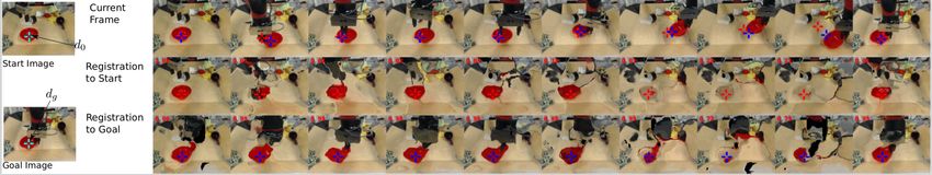
JOURNAL OF LATEX CLASS FILES, VOL. 14, NO. 8, AUGUST 2015                                                                               2

must be able to use such a model to effectively select actions
to accomplish human-specified goals. Examples of such
goals are shown in figure 1.
    We study control via prediction in the context of robotic
manipulation, formulating a model-based reinforcement
learning approach centered around prediction of raw sen-
sory observations. One of the biggest challenges in learning-
based robotic manipulation is generalization: how can we
learn models that are useful not just for a narrow range of
tasks seen during training, but that can be used to perform
new tasks with new objects that were not seen previously?
Collecting a training dataset that is sufficiently rich and
diverse is often challenging in highly-structured robotics ex-
periments, which depend on human intervention for reward
signals, resets, and safety constraints. We instead set up a
                                                                   Figure 2: Overview of visual MPC. (top) At training time,
minimally structured robotic control domain, where data is         interaction data is collected autonomously and used to train
collected by the robot via unsupervised interaction with a         a video-prediction model. (bottom) At test time, this model
wide range of objects, making it practical to collect large        is used for sampling-based planning. In this work we discuss
amounts of interaction data. The robot collects a stream           three different choices for the planning objective.
of raw sensory observations (image pixels), without any
reward signal at training time, and without the ability to
reset the environment between episodes. This setting is both       periments, including cloth manipulation and placing tasks,
realistic and necessary for studying RL in diverse real-world      a quantitative multi-task experiment assessing the perfor-
environments, as it enables automated and unattended col-          mance of our method on a wide range of distinct tasks
lection of diverse interaction experience. Since the training      with a single model, as well as a comprehensive, open-
setting affords no readily accessible reward signal, learning      sourced simulation environment to facilitate future research
by prediction presents an appealing option: the supervision        and better reproducibility. The code and videos can be found
signal for prediction is always available even in the stream       on the project webpage1 .
of unsupervised experience. We therefore propose to learn
action-conditioned predictive models directly on raw pixel         2     R ELATED W ORK
observations, and show that they can be used to accomplish         Model-based reinforcement learning. Learning a model to
a range of pixel-based manipulation tasks on a real robot in       predict the future, and then using this model to act, falls
the physical world at test-time.                                   under the general umbrella of model-based reinforcement
    The main contributions of this work are as follows.            learning. Model-based RL algorithms are generally known
We present visual MPC, a general framework for deep re-            to be more efficient than model-free methods [10], and
inforcement learning with sensory prediction models that           have been used with both low-dimensional [11] and high-
is suitable for learning behaviors in diverse, open-world          dimensional [12] model classes. However, model-based RL
environments (see figure 2). We describe deep neural net-          methods that directly operate on raw image frames have not
work architectures that are effective for predicting pixel-        been studied as extensively. Several algorithms have been
level observations amid occlusions and with novel objects.         proposed for simple, synthetic images [13] and video game
Unlike low-dimensional representations of state, specifying        environments [14], [15], [16], but have not been evaluated
and evaluating the reward from pixel predictions at test-          on generalization or in the real world, while other work
time is nontrivial: we present several practical methods           has also studied model-based RL for individual robotic
for specifying and evaluating progress towards the goal—           skills [17], [18], [19]. In contrast to these works, we place
including distances to goal pixel positions, registration to       special emphasis on generalization, studying how predictive
goal images, and success classifiers—and compare their             models can enable a real robot to manipulate previously
effectiveness and use-cases. Finally, our evaluation shows         unseen objects and solve new tasks. Several prior works
how these components can be combined to enable a real              have also sought to learn inverse models that map from
robot to perform a range of object manipulation tasks from         pairs of observations to actions, which can then be used
raw pixel observations. Our experiments include manipu-            greedily to carry out short-horizon tasks [20], [21]. However,
lation of previously unseen objects, handling multiple ob-         such methods do not directly construct longer-term plans,
jects, pushing objects around obstructions, handling clutter,      relying instead on greedy execution. In contrast, our method
manipulating deformable objects such as cloth, recovering          learns a forward model, which can be used to plan out a
from large perturbations, and grasping and maneuvering             sequence of actions to achieve a user-specified goal.
objects to user-specified locations in 3D-space. Our results       Self-supervised robotic learning. A number of recent
represent a significant advance in the generality of skills that   works have studied self-supervised robotic learning, where
can be acquired by a real robot operating on raw pixel values      large-scale unattended data collection is used to learn in-
using a single model.                                              dividual skills such as grasping [22], [23], [24], [25], push-
    This article combines and extends material from several        grasp synergies [26], or obstacle avoidance [27], [28]. In
prior conference papers [6], [7], [8], [9], presenting them in
the context of a unified system. We include additional ex-             1. For videos & code: https://sites.google.com/view/visualforesight
JOURNAL OF LATEX CLASS FILES, VOL. 14, NO. 8, AUGUST 2015                                                                                  3

contrast to these methods, our approach learns predictive
models that can be used to perform a variety of manipu-                Actions

lation skills, and does not require a success measure, event
indicator, or reward function during data collection.
                                                                                                                                   Time
Sensory prediction models. We propose to leverage sen-                 LSTM-States
sory prediction models, such as video-prediction models, to
enable large-scale self-supervised learning of robotic skills.
Prior work on action-conditioned video prediction has stud-            Transformations

ied predicting synthetic video game images [16], [29], 3D
point clouds [19], and real-world images [30], [31], [32],
using both direct autoregressive frame prediction [31], [32],          Predicted Images

[33] and latent variable models [34], [35]. Several works have
sought to use more complex distributions for future images,
for example by using pixel autoregressive models [32], [36].           True Images

While this often produces sharp predictions, the resulting
models are extremely demanding computationally. Video
prediction without actions has been studied for unstruc-           Figure 3: Computation graph of the video-prediction model.
                                                                   Time goes from left to right, at are the actions, ht are the hidden
tured videos [33], [37], [38] and driving [39], [40]. In this
                                                                   states in the recurrent neural network, F̂t+1 t is a 2D-warping
work, we extend video prediction methods that are based on
                                                                   field, It are real images, and Iˆt are predicted images, L is a
predicting a transformation from the previous image [31],          pairwise training-loss.
[40].

                                                                   different costs functions and trade-offs between them are
3   OVERVIEW
                                                                   discussed in Section 5.4.
In this section, we summarize our visual model-predictive              The model is used to plan T steps into the future,
control (MPC) method, which is a model-based reinforce-            and the first action of the action sequence that attained
ment learning approach to end-to-end learning of robotic           lowest cost, is executed. In order to correct for mistakes
manipulation skills. Our method, outlined in Figure 2,             made by the model, the actions are iteratively replanned
consists of three phases: unsupervised data collection, pre-       at each real-world time step2 ⌧ 2 {0, ..., ⌧max } following
dictive model training, and planning-based control via the         the framework of model-predictive control (MPC). In the
model at test-time.                                                following sections, we explain the video-prediction model,
Unsupervised data collection: At training time, data is col-       the planning cost function, and the trajectory optimizer.
lected autonomously by applying random actions sampled
from a pre-specified distribution. It is important that this
distribution allows the robot to visit parts of the state space
                                                                   4    V IDEO P REDICTION FOR C ONTROL
that are relevant for solving the intended tasks. For some         In visual MPC, we use a transformation-based video predic-
tasks, uniform random actions are sufficient, while for oth-       tion architecture, first proposed by Finn et al. [31]. The ad-
ers, the design of the exploration strategy takes additional       vantage of using transformation-based models over a model
care, as detailed in Sections 7 and 9.4.                           that directly generates pixels is two-fold: (1) prediction is
Model training: Also during training time, we train a video        easier, since the appearance of objects and the background
prediction model on the collected data. The model takes as         scene can be reused from previous frames and (2) the trans-
input an image of the current timestep and a sequence of           formations can be leveraged to obtain predictions about
actions, and generates the corresponding sequence of future        where pixels will move, a property that is used in several of
frames. This model is described in Section 4.                      our planning cost function formulations. The model, which
Test time control: At test time, we use a sampling-based,          is implemented as a recurrent neural network (RNN) g✓
gradient free optimization procedure, similar to a shooting        parameterized by ✓, has a hidden state ht and takes in a
method [41], to find the sequence of actions that minimizes        previous image and an action at each step of the rollout.
a cost function. Further details, including the motivation for     Future images Iˆt+1 are generated by warping the previous
this type of optimizer, can be found in Section 6.                 generated image Iˆt or the previous true image It , when
    Depending on how the goal is specified, we use one of          available, according to a 2-dimensional flow field F̂t+1 t . A
the following three cost functions. When the goal is pro-          simplified illustration of model’s structure is given in figure
vided by clicking on an object and a desired goal-position, a      3. It is also summarized in the following two equations:
pixel-distance cost-function, detailed in Section 5.1, evaluates
                                                                                          [ht+1 , F̂t+1 t ] = g✓ (at , ht , It )          (1)
how far the designated pixel is from the goal pixels. We can
specify the goal more precisely by providing a goal image                                             Iˆt+1 = F̂t+1 t ⇧ Iˆt               (2)
in addition to the pixel positions and make use of image-to-
                                                                   Here, the bilinear sampling operator ⇧ interpolates the pixel
image registration to compute a cost function, as discussed
                                                                   values bilinearly with respect to a location (x, y) and its
in Section 5.2. Finally, we show that we can specify more
                                                                   four neighbouring pixels in the image, similar to [42]. Note
conceptual tasks by providing one or several examples of
success and employing a classifier-based cost function as            2. With real-world step we mean timestep of the real-world as op-
detailed in Section 5.3. The strengths and weaknesses of           posed to predicted timesteps.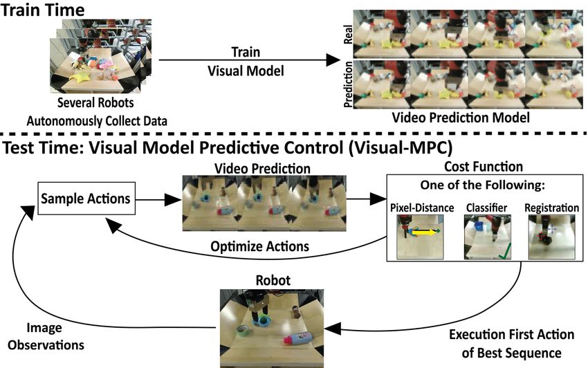
JOURNAL OF LATEX CLASS FILES, VOL. 14, NO. 8, AUGUST 2015 4
skip
arm. Hence, this model is only suitable for planning motions
48x64x2
Compositing
Masks
where the user-selected pixels are not occluded during the
5x5 3x3 3x3 3x3 3x3
manipulation, limiting its use in cluttered environments
3x3
or with multiple selected pixels. In the next section, we
Flow Field
48x64x16 24x32x32 12x16x64 6x8x128 12x16x64 24x32x32
introduce an enhanced model, which lifts this limitation by
48x64x3
48x64x2
Actions
tile
3x3
employing temporal skip connections.
6x8x5
Skip connection neural advection model. To enable ef-
Transformation
fective tracking of objects through occlusions, we can add
Convolution+
Bilinear Downsampling
temporal skip connections to the model: we now transform
Convolution+
3x3 pixels not only from the previously generated image Iˆt ,
but from all previous images Iˆ1 , ...Iˆt , including the context
Bilinear Upsampling
Conv-LSTM
Figure 4: Forward pass through the recurrent SNA model. The image I0 , which is a real image. All these transformed
red arrow indicates where the image from the first time step images can be combined to a form the predicted image
I0 is concatenated with the transformed images F̂t+1 t ⇧ Iˆt Iˆt+1 by taking a weighted sum over all transformed images,
multiplying each channel with a separate mask to produce the where the weights are given by masks Mt with the same
predicted frame for step t + 1. size as the image and a single channel:
⌧
X
Iˆt+1 = M0 (F̂t+1 0 ⇧ It ) + Mj (F̂t+1 j ⇧ Iˆj ). (4)
that, as shown in figure 3, at the first time-step the real
j=1
image is transformed, whereas at later timesteps previously
generated images are transformed in order to generate We refer to this model as the skip connection neural advection
multi-frame predictions. The model is trained with gradient model (SNA), since it handles occlusions by using temporal
descent on a `2 image reconstruction loss, denoted by L in skip connections such that when a pixel is occluded, e.g.,
figure 3. A forward pass of the RNN is illustrated in figure by the robot arm or by another object, it can still reappear
4. We use a series of stacked convolutional LSTMs and stan- later in the sequence. Transforming from all previous images
dard convolutional layers interleaved with average-pooling comes with increased computational cost, since the number
and upsampling layers. The result of this computation is the of masks and transformations scales with the number of
2 dimensional flow-field F̂t+1 t which is used to transform time-steps ⌧ . However, we found that in practice a greatly
a current image It or Iˆt . More details on the architecture are simplified version of this model, where transformations are
provided in Appendix A. applied only to the previous image and the first image of the
Predicting pixel motion. When using visual MPC with a sequence I0 , works equally well. Moreover we found that
cost-function based on start and goal pixel positions, we transforming the first image of the sequence is not necessary,
require a model that can effectively predict the 2D mo- as the model uses these pixels primarily to generate the
(1) (P )
tion of the user-selected start pixels d0 , . . . , d0 up to T image background. Therefore, we can use the first image
steps into the future3 . More details about the cost functions directly, without transformation. More details can be found
are provided in section 5. Since the model we employ in the appendix A and [7].
is transformation-based, this motion prediction capability
emerges automatically, and therefore no external pixel mo- 5 P LANNING C OST F UNCTIONS
tion supervision is required. To predict the future positions
In this section, we discuss how to specify and evaluate goals
of the designated pixel d, the same transformations used
for planning. One naı̈ve approach is to use pixel-wise error,
to transform the images are applied to the distribution
such as `2 error, between a goal image and the predicted image.
over designated pixel locations. The warping transforma-
However there is a severe issue with this approach: large
tion F̂t+1 t can be interpreted as a stochastic transition objects in the image, i.e. the arm and shadows, dominate
operator allowing us to make probabilistic predictions about such a cost; therefore a common failure mode occurs when
future locations of individual pixels: the planner matches the arm position with its position in
P̂t+1 = F̂t+1 ⇧ P̂t (3) the goal image, disregarding smaller objects. This failure
t
motivates our use of more sophisticated mechanisms for
Here, Pt is a distribution over image locations which has specifying goals, which we discuss next.
the same spatial dimension as the image. For simplicity
in notation, we will use a single designated pixel moving
5.1 Pixel Distance Cost
forward, but using multiple is straightforward. At the first
time step, the distribution P̂0 is defined as 1 at the position A convenient way to define a robot task is by choosing one
of the user-selected designated pixel and zero elsewhere. or more designated pixels in the robot’s camera view and
choosing a destination where each pixel should be moved.
The distribution P̂t+1 is normalized at each prediction step.
For example, the user might select a pixel on an object and
Since this basic model, referred to as dynamic neural
ask the robot to move it 10 cm to the left. This type of
advection (DNA), predicts images only based on the pre-
objective is general, in that it can define any object relocation
vious image, it is unable to recover shapes (e.g., objects)
task on the viewing plane. Further, success can be measured
after they have been occluded, for example by the robot
quantitatively, as detailed in section 9. Given a distribution
3. Note that when using a classifier-based cost function, we do not over pixel positions P0 , our model predicts distributions
require the model to output transformations. over its positions Pt at time t 2 {1, . . . , T }. One way of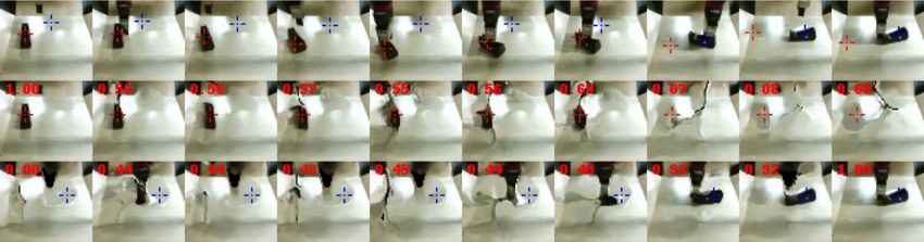
JOURNAL OF LATEX CLASS FILES, VOL. 14, NO. 8, AUGUST 2015                                                                                                                      5

               !#                     !"             !$
                                                                        &%
                                                                                 '          !"#←%
                          …                   …
                                                                        &#
                                                                                                                                                                 loss
                                                                                                                   '#      )            !"#$%←%        '(#$%            '#$%

                                                                                                                               shared
                         &'#←"               &'$←"                      &%
                                                                                 '          !"#←%                 '#$%     )            !"#←#$%         '(#
                                                                                                                                                                 loss
                                                                                                                                                                         '#
                                                                        &#
               !%#                    !"             !%$
Figure 5: Closed loop control is achieved by registering the            (a) Testing usage.                                (b) Training usage.
current image It globally to the first frame I0 and the goal          Figure 6: (a) At test time the registration network registers
image Ig . In this example registration to I0 succeeds while          the current image It to the start image I0 (top) and goal
registration to Ig fails since the object in Ig is too far away.
                                                                      image Ig (bottom), inferring the flow-fields F̂0 t and F̂g t . (b)
                                                                      The registration network is trained by warping images from
                                                                      randomly selected timesteps along a trajectory to each other.

defining the cost per time-step ct is by using the expected
Euclidean distance to the goal point dg , which is straight-          vector field with the same size as the image, that describes
forward to calculate from Pt and g , as follows:                      the relative motion for every pixel between the two frames.
              X           X              h          i
       c=          ct =         Edˆt ⇠Pt kdˆt dg k2      (5)                    F̂0   t   = R(It , I0 )                   F̂g       t   = R(It , Ig )                         (6)
             t=1,...,T           t=1,...,T
                                                                      The flow map F̂0 t can be used to warp the image of the
The per time-step costs ct are summed together giving                 current time step t to the start image I0 , and F̂g t can be
the overall planing objective c. The expected distance to             used to warp from It to Ig (see Figure 5 for an illustration).
the goal provides a smooth planning objective and enables             There is no difference to the warping operation used in the
longer-horizon tasks, since this cost function encourages             video prediction model, explained in section 4, equation 2:
movement of the designated objects into the right direction
                                                                                  Iˆ0 = F̂0         t   ⇧ It               Iˆg = F̂g              t   ⇧ It                    (7)
for each step of the execution, regardless of whether the
goal-position can be reached within T time steps or not.              In essence for a current image F̂0 t puts It in correspon-
This cost also makes use of the uncertainty estimates of              dence with I0 , and F̂g t puts It in correspondence with
the predictor when computing the expected distance to                 Ig . The motivation for registering to both I0 and Ig is to
the goal. For multi-objective tasks with multiple designated          increase accuracy and robustness. In principle, registering to
pixels d(i) the costs are summed to together, and optionally          either I0 or Ig is sufficient. While the registration network is
weighted according to a scheme discussed in subsection 5.2.           trained to perform a global registration between the images,
                                                                      we only evaluate it at the points d0 and dg chosen by the
                                                                      user. This results in a cost function that ignores distractors.
5.2   Registration-Based Cost
                                                                      The flow map produced by the registration network is used
We now propose an improvement over using pixel dis-                   to find the pixel locations corresponding to d0 and dg in the
tances. When using pixel distance cost functions, it is neces-        current frame:
                                                  (1)          (P )
sary to know the current location of the object, d0 , . . . , d0
                                                                             dˆ0,t = d0 + F̂0           t (d0 )          dˆg,t = dg + F̂g                     t (dg )         (8)
at each replanning step, so that the model can predict the
positions of this pixel from the current step forward. To                 For simplicity, we describe the case with a single des-
update the belief of where the target object currently is,            ignated pixel. In practice, instead of a single flow vector
we propose to register the current image to the start and             F̂0 t (d0 ) and F̂g t (dg ), we consider a neighborhood of
optionally also to a goal image, where the designated pixels          flow-vectors around d0 and dg and take the median in the
are marked by the user. Adding a goal image can make                  x and y directions, making the registration more stable.
visual MPC more precise, since when the target object is              Figure 7 visualizes an example tracking result while the
close to the goal position, registration to the goal-image            gripper is moving an object.
greatly improves the position estimate of the designated              Registration-based pixel distance cost. Registration can fail
pixel. Crucially, the registration method we introduce is self-       when distances between objects in the images are large.
supervised, using the same exact data for training the video          During a motion, the registration to the first image typically
prediction model and for training the registration model.             becomes harder, while the registration to the goal image
This allows both models to continuously improve as the                becomes easier. We propose a mechanism that estimates
robot collects more data.                                             which image is registered correctly, allowing us to utilize
Test time procedure. We will first describe the registration          only the successful registration for evaluating the planning
scheme at test time (see Figure 6(a)). We separately register         cost. This mechanism gives a high weight i to pixel dis-
the current image It to the start image I0 and to the goal            tance costs ci associated with a designated pixel dˆi,t that
image Ig by passing it into the registration network R, im-           is tracked successfully and a low, ideally zero, weight to
plemented as a fully-convolutional neural network. The reg-           a designated pixel where the registration is poor. We use
istration network produces a flow map F̂0 t 2 RH⇥W ⇥2 , a             the photometric distance between the true frame and the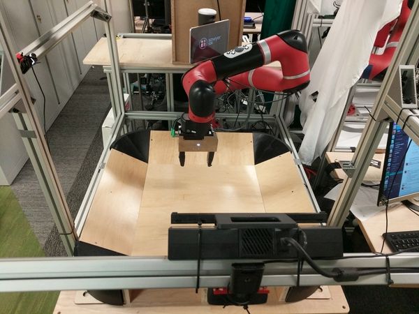
JOURNAL OF LATEX CLASS FILES, VOL. 14, NO. 8, AUGUST 2015                                                                               6

Figure 7: Outputs of registration network. The first row shows the timesteps from left to right of a robot picking and moving a
red bowl, the second row shows each image warped to the initial image via registration, and the third row shows the same for the
goal image. A successful registration in this visualization would result in images that closely resemble the start- or goal image. In
the first row, the locations where the designated pixel of the start image d0 and the goal image dg are found are marked with red
and blue crosses, respectively. It can be seen that the registration to the start image (red cross) is failing in the second to last time
step, while the registration to the goal image (blue cross) succeeds for all time steps. The numbers in red, in the upper left corners
indicate the trade off factors between the views and are used as weighting factors for the planning cost. (Best viewed in PDF)

warped frame evaluated at d0,i and dg,i as an estimate for               between Iˆt and It and Iˆt+h and It+h , in addition to a
local registration success. A low photometric error indicates            smoothness regularizer that penalizes abrupt changes in the
that the registration network predicted a flow vector leading            outputted flow-field. The details of this loss function follow
to a pixel with a similar color, thus indicating warping                 prior work [43]. We found that gradually increasing the tem-
success. However this does not necessarily mean that the                 poral distance h between the images during training yielded
flow vector points to the correct location. For example, there           better final accuracy, as it creates a learning curriculum. The
could be several objects with the same color and the network             temporal distance is linearly increased from 1 step to 8 steps
could simply point to the wrong object. Letting Ii (di ) denote          at 20k SGD steps. In total 60k iterations were taken.
the pixel value in image Ii for position di , and Iˆi (di )                  The network R is implemented as a fully convolutional
denote the corresponding pixel in the image warped by the                network taking in two images stacked along the channel di-
registration function, we can define the general weighting               mension. First the inputs are passed into three convolutional
factors i as:                                                            layers each followed by a bilinear downsampling operation.
                                                                         This is passed into three layers of convolution each followed
                         ||Ii (di ) Iˆi (di )||2 1                       by a bilinear upsampling operation (all convolutions use
                  i   = PN                             .           (9)
                         j ||Ij (dj )   Iˆj (dj )||2 1                   stride 1). By using bilinear sampling for increasing or de-
                                                                         creasing image sizes we avoid artifacts that are caused by
where Iˆi = F̂i t ⇧ It . The MPC cost is computed as the                 strided convolutions and deconvolutions.
average of the costs ci weighted by i , where each ci is the
expected distance (see equation 5) between the registered
point dˆi,t and the                                                      5.3 Classifier-Based Cost Functions
                 P goal point dg,i . Hence, the cost used for
planning is c = i i ci . In the case of the single view model            An alternative way to define the cost function is with a
and a single designated pixel, the index i iterates over the             goal classifier. This type of cost function is particularly well-
start and goal image (and N = 2).                                        suited for tasks that can be completed in multiple ways.
    The proposed weighting scheme can also be used with                  For example, for a task of rearranging a pair objects into
multiple designated pixels, as used in multi-task settings               relative positions, i.e. pushing the first object to the left of
and multi-view models, which are explained in section 8.                 the second object, the absolute positions of the objects do
The index i then also loops over the views and indices of                not matter nor does the arm position. A classifier-based cost
the designated pixels.                                                   function allows the planner to discover any of the possible
Training procedure. The registration network is trained on               goal states.
the same data as the video prediction model, but it does not                 Unfortunately, a typical image classifier will require a
share parameters with it.4 Our approach is similar to the                large amount of labeled examples to learn, and we do
optic flow method proposed by [43]. However, unlike this                 not want to collect large datasets for each and every task.
prior work, our method computes registrations for frames                 Instead, we aim to learn a goal classifier from only a few
that might be many time steps apart, and the goal is not to              positive examples, using a meta-learning approach. A few
extract optic flow, but rather to determine correspondences              positive examples of success are easy for people to provide
between potentially distant images. For training, two im-                and are the minimal information needed to convey a goal.
ages are sampled at random times steps t and t + h along                     Formally, we consider a goal classifier ŷ = f (o), where
the trajectory and the images are warped to each other in                o denotes the image observation, and ŷ 2 [0, 1] indicates
both directions.                                                         the predicted probability of the observation being of a
                                                                         successful outcome of the task. Our objective is to infer a
      Iˆt = F̂t   t+h   ⇧ It+h        Iˆt+h = F̂t+h    t   ⇧ It   (10)   classifier for a new task Tj from a few positive examples of
                                                                         success, which are easy for a user to provide and encode
The network, which outputs F̂t t+h and F̂t+h t , see Fig-
                                                                         the minimal information needed to convey a task. In other
ure 6 (b), is trained to minimize the photometric distance
                                                                         words, given a dataset Dj+ of K examples of successful end
 4. In principle, sharing parameters with the video prediction model     states for a new task Tj : Dj := {(ok , 1)|k = 1...K}j , our
might be beneficial, but this is left for future work.                   goal is to infer a classifier for task Tj .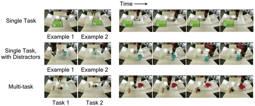
JOURNAL OF LATEX CLASS FILES, VOL. 14, NO. 8, AUGUST 2015                                                                                  7

                                                                          classifier conservatively by thresholding the predictions so
                                                                          that reward is only given for confident successes. Below this
                                                                          threshold, we give a reward of 0 and above this threshold,
                                                                          we provide the predicted probability as the reward.
                                                                          Training time procedure. During meta-training, we explic-
                                                                          itly train for the ability to infer goal classifiers for the set of
                                                                          training tasks, {Ti }. We assume a small dataset Di for each
                                                                          task Ti , consisting of both positive and negative examples:
                                                                          Di := {(on , yn )|n = 1...N }i . To learn the initial parameters
                                                                          ✓, we optimize the following objective using Adam [46]:
Figure 8: We propose a framework for quickly specifying visual                               X        X
goals. Our goal classifier is meta-trained with positive and                            min                   L(yn , f (on ; ✓i0 ))
negative examples for diverse tasks (left), which allows it to                           ✓
                                                                                              i   (on ,yn )2Ditest
meta-learn that some factors matter for goals (e.g., relative
positions of objects), while some do not (e.g. position of the                In our experiments, our classifier is represented by a con-
arm). At meta-test time, this classifier can learn goals for new          volutional neural network, consisting of three convolutional
tasks from a few of examples of success (right - the goal is to           layers, each followed by layer normalization and a ReLU
place the fork to the right of the plate). The cost can be derived        non-linearity. After the final convolutional layer, a spatial
from the learned goal classifier for use with visual MPC.
                                                                          soft-argmax operation extracts spatial feature points, which
                                                                          are then passed through fully-connected layers.
Meta-learning for few-shot goal inference. To solve the
above problem, we propose learning a few-shot classifier
that can infer the goal of a new task from a small set of                 5.4 When to Use Which Cost Function?
goal examples, allowing the user to define a task from a few              We have introduced three different forms of cost function,
examples of success. To train the few-shot classifier, we first           pixel distance based cost functions with and without regis-
collect a dataset of both positive and negative examples for              tration, as well as classifier-based cost functions. Here we
a wide range of tasks. We then use this data to learn how                 discuss the relative strengths and weaknesses of each.
to learn goal classifiers from a few positive examples. Our                   Pixel distance based cost functions have the advantage
approach is illustrated in Figure 8.                                      that they allow moving objects precisely to target locations.
    We build upon model-agnostic meta-learning                            They are also easy to specify, without requiring any example
(MAML) [44], which learns initial parameters ✓ for                        goal images, and therefore provide an easy and fast user
model f that can efficiently adapt to a new task with one or              interface. The pixel distance based cost function also has
a few steps of gradient descent. Grant et al. [45] proposed               a high degree of robustness against distractor objects and
an extension of MAML, referred to as concept acquisition                  clutter, since the optimizer can ignore the values of other
through meta-learning (CAML), for learning to learn new                   pixels; this is important when targeting diverse real-world
concepts from positive examples alone. We apply CAML                      environments. By incorporating an image of the goal, we
to the setting of acquiring goal classifiers from positive                can also add a registration mechanism to allow for more
examples, using a meta-training data with both positive                   robust closed-loop control, at the cost of a more significant
and negative examples. The result of the meta-training                    burden on the user.
procedure is an initial set of parameters that can be used to                 The classifier-based cost function allows for solving more
learn new goal classifiers at test time.                                  abstract tasks since it can capture invariances, such as
Test time procedure. At test time, the user provides a                    the position of the arm, and settings where the absolute
dataset Dj+ of K examples of successful end states for a new              positions of an object is not relevant, such as positioning
task Tj : Dj := {(ok , 1)|k = 1...K}j , which are then used to            a cup in front of a plate, irrespective of where the plate
infer a task-specific goal classifier Cj . In particular, the meta-       is. Providing a few example images takes more effort than
learned parameters ✓ are updated through gradient descent                 specifying pixel locations but allows a broader range of goal
to adapt to task Tj :                                                     sets to be specified.

                                          X
Cj (o) = f (o; ✓j0 ) = f o; ✓    ↵r✓                  L(yn , f (on ; ✓)   6   T RAJECTORY O PTIMIZER
                                      (on ,yn )2Dj+                       The role of the optimizer is to find actions sequences a1:T
                                                                          that minimize the sum of the costs c1:T along the planning
    where L is the cross-entropy loss function, ↵ is the                  horizon T . We use a simple stochastic optimization proce-
step size, and ✓0 denotes the parameters updated through                  dure for this, based on the cross-entropy method (CEM), a
gradient descent on task Tj .                                             gradient-free optimization procedure. CEM consists of iter-
    During planning, the learned classifier Cj takes as input             atively resampling action sequences and refitting Gaussian
an image generated by the video prediction model and out-                 distributions to the actions with the best predicted cost.
puts the predicted probability of the goal being achieved for                 Although a variety of trajectory optimization methods
the task specified by the few examples of success. To convert             may be suitable, one advantage of the stochastic optimiza-
this into a cost function, we treat the probability of success            tion procedure is that it allows us to easily ensure that
as the planning cost for that observation. To reduce the effect           actions stay within the distribution of actions the model
of false positives and mis-calibrated predictions, we use the             encountered during training. This is crucial to ensure that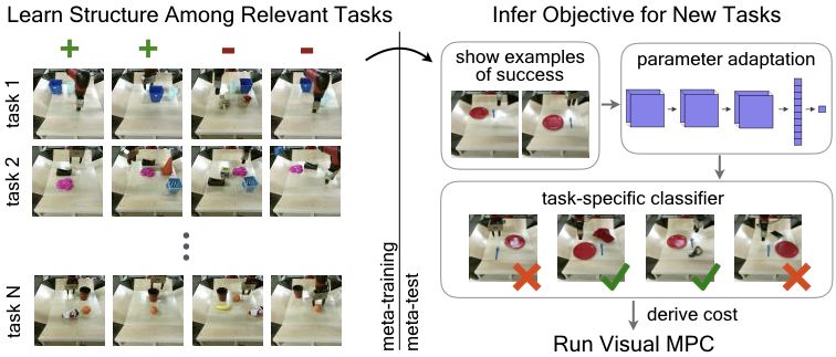
JOURNAL OF LATEX CLASS FILES, VOL. 14, NO. 8, AUGUST 2015                                                                                 8

Algorithm 1 Planning in Visual MPC                                 the appendix). In our experiments, we evaluate our method
 1: Inputs: Predictive model g , planning cost function c          using data obtained both with and without the grasping
 2: for t = 0...T     1 do                                         reflex, evaluating both purely non-prehensile and combined
 3:     for i = 0...niter 1 do                                     prehensile and non-prehensile manipulation.
 4:         if i == 0 then
                                             (m)
 5:             Sample M action sequences {at:t+H 1 } from
              N (0, I) or custom sampling distribution
                                                                   8     M ULTI -V IEW V ISUAL MPC
 6:       else                                                     The visual MPC algorithm
                                              (m)
 7:           Sample M action sequences at:t+H 1 from              as described so far is only     Robot
              N (µ(i) , ⌃(i) )                                     able to solve manipulation
 8:       Check if sampled actions are within                      tasks specified in 2D, like     Webcams

          admissible range, otherwise resample.                    rearranging objects on the
                                                                                                   Viewing
 9:
                                                       (m)
          Use g to predict future image sequences Iˆt:t+H 1        table. However, this can        Direction

                                            (m)                    impose severe limitations;
          and probability distributions P̂t:t+H 1
                                                                   for example, a task such as     Object Bin
10:       Evaluate action sequences using a cost function c
                                                                   lifting an object to a partic-
11:       Fit a diagonal Gaussian to the k action samples
                                                                   ular position in 3D cannot
          with lowest cost, yielding µ(i) , ⌃(i)
                                                                   be fully specified with a Figure 9: Robot setup, with 2
12:     Apply first action of best action sequence to robot        single view, since it would standard web-cams arranged at
                                                                   be ambiguous. We use a different viewing angles.
                                                                   combination of two views,
the model does not receive out-of-distribution inputs and          taken from two cameras arranged appropriately, to jointly
makes valid predictions. Algorithm 1 illustrates the plan-         define a 3D task. Figure 9 shows the robot setup, includ-
ning process. In practice this can be achieved by defining         ing two standard webcams observing the workspace from
admissible ranges for each dimension of the action vector          different angles. The registration method described in the
and rejecting a sample if it is outside of the admissible range.   previous section is used separately per view to allow for
   In the appendix C we present a few improvements to the          dynamic retrying and solving temporally extended tasks.
CEM optimizer for visual MPC.                                      The planning costs from each view are combined using
                                                                   weighted averaging where the weights are provided by the
                                                                   registration network (see equation 9). Rows 5 and 6 of figure
7     C USTOM ACTION S AMPLING D ISTRIBUTIONS
                                                                   12 show a 3D object positioning task, where an object needs
When collecting data by sampling from simple distri-               to be positioned at a particular point in 3D space. This task
butions, such as a multivariate Gaussian, the skills that          needs two views to be fully specified.
emerged were found to be generally restricted to pushing
and dragging objects. This is because with simple distri-
butions, it is very unlikely to visit states like picking up       9     E XPERIMENTAL E VALUATION
and placing of objects or folding cloth. Not only would the        In this section we present both qualitative and quantitative
model be imprecise for these kinds of states, but also during      performance evaluations of visual MPC on various manip-
planning it would be unlikely to find action sequences that        ulation tasks assessing the degree of generalization and
grasp an object or fold an item of clothing. We therefore          comparing different prediction models and cost functions
explore how the sampling distribution used both in data            and with a hand-crafted baseline. In Figures 1 and 12 we
collection and sampling-based planning can be changed              present a set of qualitative experiments showing that visual
to visit these, otherwise unlikely, states more frequently,        MPC trained fully self-supervised is capable of solving a
allowing more complex behavior to emerge.                          wide range of complex tasks. Videos for the qualitative
    To allow picking up and placing of objects as well as          examples are at the following webpage5 . In order to perform
folding of cloth to occur more frequently, we incorporate          quantitative comparisons, we define a set of tasks where the
a simple “reflex” during data collection, where the gripper        robot is required to move object(s) into a goal configuration.
automatically closes, when the height of the wrist above           For measuring success, we use a distance-based evaluation
the table is lower than a small threshold. This reflex is          where a human annotates the positions of the objects after
inspired by the palmar reflex observed in infants [47].            pushing allowing us to compute the remaining distance to
With this primitive, when collecting data with rigid objects       the goal.
about 20% of trajectories included some sort of grasp. For
deformable objects such as towels and cloth, this primitive
helps increasing the likelihood of encountering states where       9.1 Comparing Video Prediction Architectures
cloths are folded. We found that the primitive can be slightly     We first aim to answer the question: Does visual MPC
adapted to avoid cloths becoming tangled up. More details          using the occlusion-aware SNA video prediction model that
are provided in Appendix B.                                        includes temporal skip connections outperform visual MPC
    It is worth noting that, other than this reflex, no            with the dynamic neural advection model (DNA) [6] without
grasping-specific or folding-specific engineering was ap-          temporal skip-connections?
plied to the policy, allowing a joint pushing, grasping and
folding policy to emerge through planning (see figure 16 in            5. Videos & code: https://sites.google.com/view/visualforesight/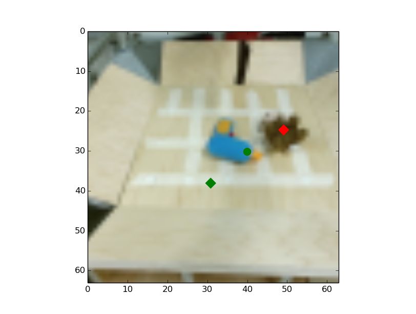
JOURNAL OF LATEX CLASS FILES, VOL. 14, NO. 8, AUGUST 2015                                                                         9

                       moved imp.         stationary imp.
                    ± std err. of mean   ± std err. of mean

         DNA [6]        0.83 ±0.25           -1.1 ± 0.2
         SNA            10.6 ± 0.82          -1.5 ± 0.2

Table 1: Results for multi-objective pushing on 8 object/goal
configurations with 2 seen and 2 novel objects. Values indi-
cate improvement in distance from starting position, higher
is better. Units are pixels in the 64x64 images.

                                               Short      Long     Figure 10: Object arrangement performance of our goal classi-
                                                                   fier with distractor objects and with two tasks. The left shows a
        Visual MPC + predictor propagation     83%        20%      subset of the 5 positive examples that are provided for inferring
        Visual MPC + OpenCV tracking           83%        45%
        Visual MPC + registration network      83%        66%
                                                                   the goal classifier(s), while the right shows the robot executing
                                                                   the specified task(s) via visual planning.

Table 2: Success rate for long-distance pushing experiment with    the trajectory the object behaves differently than expected,
20 different object/goal configurations and short-distance ex-     it moves downwards instead of to the right. However the
periment with 15 object/goal configurations. Success is defined
                                                                   system recovers from the initial failure and still pushes the
as bringing the object closer than 15 pixels to the goal, which
corresponds to around 7.5cm.                                       object to the goal.
                                                                       The next question we investigate is: How much does
                                                                   tracking the target object using the learned registration
    To examine whether our skip-connection model (SNA)             matter for short horizon versus long horizon tasks? In this
helps with handling occlusions, we devised a task that             experiment, we disable the gripper control, which requires
requires the robot to push one object, while keeping another       the robot to push objects to the target. We compare two vari-
object stationary. When the stationary object is in the way,       ants of updating the positions of the designated pixel when
the robot must move the target object around it. This is           using a pixel-distance based cost function. The first is a cost
illustrated on the left side of Figure 17 in the appendix.         function that uses our registration-based method, trained in
While pushing the target object, the gripper may occlude           a fully self-supervised fashion, and the second is with a cost
the stationary object, and the task can only be performed          function that uses off-the shelf tracking from OpenCV [48].
successfully if the model can make accurate predictions            Additionally we compare to visual MPC, which uses the
through this occlusion. These tasks are specified by selecting     video-prediction model’s own prior predictions to update
one starting pixel on the target object, a goal pixel location     the current position of the designated pixel, rather than
for the target object, and commanding the obstacle to remain       tracking the object with registration or tracking.
stationary by selecting the same pixel on the obstacle for             We evaluate our method on 20 long-distance and 15
both start and goal.                                               short-distance pushing tasks. For long distance tasks the
    We use four different object arrangements with two             initial distance between the object and its goal position is
training objects and two objects that were not seen during         30cm while for short distance tasks it is 15cm. Table 2 lists
training. We find that, in most cases, the SNA model is            quantitative comparisons showing that on the long distance
able to find a valid trajectory, while the DNA model, that         experiment visual MPC using the registration-based cost not
is not able to handle occlusion, is mostly unable to find a        only outperforms prior work [7], but also outperforms the
solution. The results of our quantitative comparisons are          hand-designed, supervised object tracker [48]. By contrast,
shown in Table 1, indicating that temporal skip-connections        for the short distance experiment, all methods perform com-
indeed help with handling occlusion in combined pushing            parably. Thus, theses results demonstrate the importance
and obstacle avoidance tasks.                                      of tracking the position of the target object for long-horizon
                                                                   tasks, while for short-horizon tasks object tracking appears
9.2   Evaluating Registration-Based Cost Functions                 to be irrelevant.
In this section we ask: How important is it to update the
model’s belief of where the target objects currently are? We       9.3 Evaluating Classifier-Based Cost Function
first provide two qualitative examples: In example (5)-(6)         The goal of the classifier-based cost function is to provide
of Figure 12 the task is to bring the stuffed animal to a          an easy way to compute an objective for new tasks from
particular location in 3D-space on the other side of the arena.    a few observations of success for that task, so we compare
To test the system’s reaction to perturbations that could          our approach to alternative and prior methods for doing so
be encountered in open-world settings, during execution            under the same assumptions: pixel distance and latent space
a person knocks the object out of the robot’s hand (in the         distance. In the latter, we measure the distance between
3rd frame). The experiment shows that visual MPC is able           the current and goal observations in a learned latent space,
to naturally perform a new grasp attempt and bring the             obtained by training an autoencoder (DSAE) [17] on the
object to the goal. This trajectory is easier to view in the       same data used for our classifier. Since we are considering a
supplementary video.                                               different form of task specification incompatible with user-
    In Figure 15 in the appendix, the task is to push the bottle   specified pixels, we do not compare the classifier-based cost
to the point marked with the green dot. In the beginning of        function to the cost function based on designated pixels.
JOURNAL OF LATEX CLASS FILES, VOL. 14, NO. 8, AUGUST 2015 10
are shown in Figure 1 and 12. Task 1 in Figure 1 shows
a “placing task” where an object needs to be grasped and
placed onto a plate while not displacing the plate. Task 2
is an object rearrangement tasks. The example shown in
Task 4 and all examples in Figure 10 show relative object
rearrangement tasks. Examples 5 and 6 show the same 3D
object positioning tasks from different views. In Task 7, the
goal is to move the black object to the goal location while
avoiding the obstacle in the middle which is marked with a
Figure 11: Quantitative performance of visual planning for designated- and goal pixel. We also demonstrate that visual
object rearrangement tasks across different goal specification MPC – without modifications to the algorithm – solves tasks
methods: our meta-learned classifier, DSAE [17], and pixel involving deformable objects such as a task where a towel
error. Where possible, we include break down the cause of needs to be wrapped around an object (Task 3), or folding
failures into errors caused by inaccurate prediction or planning a pair of shorts (Task 8). To the best of our knowledge
and those caused by an inaccurate goal classifier. this is the first algorithm for robotic manipulation handling
both rigid and deformable objects. For a full illustration of
To collect data for meta-training the classifier, we ran- each of these tasks, we encourage the reader to watch the
domly select a pair of objects from our set of training supplementary video.
objects, and position them in many different relative po- The generality of visual MPC mainly stems from two
sitions, recording the image for each configuration. Each components — the generality of the visual dynamics model
task corresponds to a particular relative positioning of two and the generality of the task definition. We found that the
objects, e.g. the first object to the left of the second, and we dynamics model often generalizes well to objects outside
construct positive and negative examples for each task by of the training set, if they have similar properties to the
labeling the aforementioned images. We randomly position objects it was trained with. For example, Task 8 in Figure
the arm in each image, as it is not a determiner of task 12 shows the model predicting a pair of shorts being folded.
success. A good classifier should ignore the position of the We observed that a model, which was only provided videos
arm. We also include randomly-positioned distractor objects of towels during training, generalized to shorts, although
in about a third of the collected images. it had never seen them before. In all of the qualitative
We evaluate the classifier-based cost function in three examples, the predictions are performed by the same model.
different experimental settings. In the first setting, the goal is We found that the model sometimes exhibits confusion
to arrange two objects into a specified relative arrangement. about whether an object follows the dynamics of a cloth
The second setting is the same, but with distractor objects or rigid objects, which is likely caused by a lack of training
present. In the final and most challenging setting, the goal data in the particular regime. To overcome this issue we add
is to achieve two tasks in sequence. We provide positive a binary token to the state vector indicating whether the
examples for both tasks, infer the classifier for both, perform object in the bin is hard or soft. We expect that adding more
MPC for the first task until completion, followed by MPC for training data would remove the need for this indicator and
the second task. The arrangements of the evaluation tasks allow the model to infer material properties directly from
were chosen among the eight principal directions (N, NE, E, images.
SE, etc.). To evaluate the ability to generalize to new goals The ability to specify tasks in multiple different ways
and settings, we use novel, held-out objects for all of the adds to the flexibility of the proposed system. Using desig-
task and distractor objects in our evaluation. nated pixels, object positioning tasks can be defined in 3D
We qualitatively visualize the tasks in Figure 10. On space, as shown in Task 1 and 2 in Figure 1 and task 5-6 in
the left, we show a subset of the five images provided to Figure 12. When adding a goal image, the positioning accu-
illustrate the task(s), and on the left, we show the motions racy can be improved by utilizing the registration scheme
performed by the robot. We see that the robot is able to discussed in Section 5.2. For tasks where we care about
execute motions which lead to a correct relative positioning relative rather than absolute positioning, a meta-learned
of the objects. We quantitatively evaluate the three cost classifier can be used, as discussed in Section 5.3.
functions across 20 tasks, including 10 unique object pairs. Next, we present a quantitative evaluation to answer
A task was considered successfully completed if more than the following question: How does visual MPC compare to
half of the object was correctly positioned relative to the a hand-engineered baseline on a large number of diverse
other. The results, shown in Figure 11, indicate that the tasks? For this comparison, we engineered a simple trajec-
distance-based metrics struggle to infer the goal of the task, tory generator to perform a grasp at the location of the initial
while our approach leads to substantially more successful designated pixel, lift the arm, and bring it to the position
behavior on average. of the goal pixel. Camera calibration was performed to
carry out the necessary conversions between image-space
and robot work-space coordinates, which was not required
9.4 Evaluating Multi-Task Performance for our visual MPC method. For simplicity, the baseline
One of the key motivations for visual MPC is to build a controller executes in open loop. Therefore, to allow for a
system that can solve a wide variety of different tasks, in- fair comparison, visual MPC is also executed open-loop, i.e.
volving completely different objects, physics and, objectives. no registration or tracking is used. Altogether we selected 16
Examples for tasks that can be solved with visual MPC tasks, including the qualitative examples presented earlier.JOURNAL OF LATEX CLASS FILES, VOL. 14, NO. 8, AUGUST 2015 11
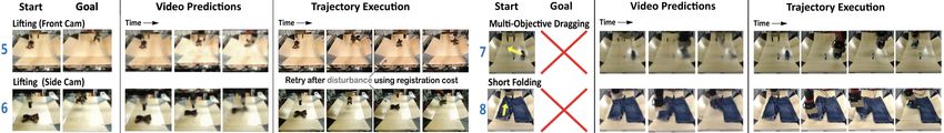
Figure 12: Visual MPC successfully solves a wide variety of tasks including multi-objective tasks, such as placing an object
on a plate (row 5 and 6), object positioning with obstacle avoidance (row 7) and folding shorts (row 8). Zoom in on PDF.
% of Trials with picking and placing, and cloth-folding tasks – all within a
Final Pixel Distance < 15 single framework.
Visual MPC 75% Limitations. The main limitations of the presented frame-
Calibrated Camera Baseline 18.75 % work are that all target objects need to be visible throughout
execution, it is currently not possible to handle partially
Table 3: Results for a multi-task experiment of 10 hard object observed domains. This is especially important for tasks
pushing and grasping tasks, along with 6 cloth folding that require objects to be brought into occlusion (or taken
tasks, evaluating using a single model. Values indicate the out of occlusion), for example putting an object in a box and
percentage of trials that ended with the object pixel closer closing it. Another limitation is that the tasks are still of only
than 15 pixels to the designated goal. Higher is better. medium duration and usually only touch one or two objects.
Longer-term planning remains an open problem. Lastly, the
fidelity of object positioning is still significantly below what
The quantitative comparison is shown in Table 3, illustrating humans can achieve.
that visual MPC substantially outperforms this baseline. Possible future directions. The key advantage of a model-
Visual MPC succeeded for most of the tasks. While the based deep-reinforcement learning algorithm like visual
baseline succeeded for some of the cloth folding tasks, it MPC is that it generalizes to tasks it has never encountered
failed for almost all of the object relocation tasks. This before. This makes visual MPC a good candidate for a
indicates that an implicit understanding of physics, as cap- building block of future robotic manipulation systems that
tured by our video prediction models, is indeed essential will be able solve an even wider range of complex tasks with
for performing this diverse range of object relocation and much longer horizons.
manipulation tasks, and the model must perform non-trivial
physical reasoning beyond simply placing and moving the
end-effector. R EFERENCES
9.5 Discussion of Experimental Results [1] G. Tesauro, “Temporal difference learning and td-gammon,” Com-
munications of the ACM, vol. 38, no. 3, pp. 58–68, 1995.
Generalization to many distinct tasks in visually diverse [2] V. Mnih, K. Kavukcuoglu, D. Silver, A. Graves, I. Antonoglou,
settings is arguably one of the biggest challenges in rein- D. Wierstra, and M. Riedmiller, “Playing atari with deep reinforce-
ment learning,” arXiv:1312.5602, 2013.
forcement learning and robotics today. While deep learning [3] S. Levine, C. Finn, T. Darrell, and P. Abbeel, “End-to-end learning
has relieved us from much of the problem-specific engineer- of deep visuomotor policies,” Journal of Machine Learning Research
ing, most of the works either require extensive amounts (JMLR), 2016.
of labeled data or focus on the mastery of single tasks [4] D. Silver, T. Hubert, J. Schrittwieser, I. Antonoglou, M. Lai,
A. Guez, M. Lanctot, L. Sifre, D. Kumaran, T. Graepel et al., “Mas-
while relying on human-provided reward signals. From the tering chess and shogi by self-play with a general reinforcement
experiments with visual MPC, especially the qualitative ex- learning algorithm,” arXiv:1712.01815, 2017.
amples and the multi-task experiment, we can conclude that [5] A. Bubic, D. Y. Von Cramon, and R. Schubotz, “Prediction, cogni-
visual MPC generalizes to a wide range of tasks it has never tion and the brain,” Frontiers in Human Neuroscience, 2010.
[6] C. Finn and S. Levine, “Deep visual foresight for planning robot
seen during training. This is in contrast to many model- motion,” in International Conference on Robotics and Automation
free approaches for robotic control which often struggle to (ICRA), 2017.
perform well on novel tasks. Most of the generalization [7] F. Ebert, C. Finn, A. X. Lee, and S. Levine, “Self-supervised visual
planning with temporal skip connections,” Conference on Robot
performance is likely a result of large-scale self-supervised
Learning (CoRL), 2017.
learning, which allows to acquire a rich, task-agnostic dy- [8] F. Ebert, S. Dasari, A. X. Lee, S. Levine, and C. Finn, “Robust-
namics model of the environment. ness via retrying: Closed-loop robotic manipulation with self-
supervised learning,” Conference on Robot Learning (CoRL), 2018.
[9] A. Xie, A. Singh, S. Levine, and C. Finn, “Few-shot goal inference
10 C ONCLUSION for visuomotor learning and planning,” Conference on Robot Learn-
ing (CoRL), 2018.
We presented an algorithm that leverages self-supervision [10] M. P. Deisenroth, G. Neumann, J. Peters et al., “A survey on policy
from visual prediction to learn a deep dynamics model on search for robotics,” Foundations and Trends R in Robotics, 2013.
images, and show how it can be embedded into a planning [11] M. Deisenroth and C. E. Rasmussen, “Pilco: A model-based and
data-efficient approach to policy search,” in International Conference
framework to solve a variety of robotic control tasks. We on Machine Learning (ICML), 2011.
demonstrate that visual model-predictive control is able to [12] I. Lenz and A. Saxena, “Deepmpc: Learning deep latent features
successfully perform multi-object manipulation, pushing, for model predictive control,” in In RSS. Citeseer, 2015.You can also read