Kindergarden quantum mechanics graduates
←
→
Page content transcription
If your browser does not render page correctly, please read the page content below
Kindergarden quantum mechanics graduates
                                                   ...or how I learned to stop gluing LEGO together and love the ZX-calculus

                                                      Bob Coecke† , Dominic Horsman? , Aleks Kissinger‡ , Quanlong Wang†
                                                                       †
                                                                        Cambridge Quantum Computing Ltd.
arXiv:2102.10984v1 [quant-ph] 22 Feb 2021

                                                                 bob.coecke/harny.wang@cambridgequantum.com
                                                              ?
                                                                 Université Grenoble Alpes. dom.horsman@gmail.com
                                                               ‡
                                                                 Oxford University. aleks.kissinger@cs.ox.ac.uk

                                                                                     February 23, 2021

                                                                                          Abstract
                                                     This paper is a ‘spiritual child’ of the 2005 lecture notes Kindergarten Quantum Mechan-
                                                 ics [23], which showed how a simple, pictorial extension of Dirac notation allowed several
                                                 quantum features to be easily expressed and derived, using language even a kindergartner
                                                 can understand. Central to that approach was the use of pictures and pictorial transforma-
                                                 tion rules to understand and derive features of quantum theory and computation. However,
                                                 this approach left many wondering ‘where’s the beef?’ In other words, was this new ap-
                                                 proach capable of producing new results, or was it simply an aesthetically pleasing way to
                                                 restate stuff we already know?
                                                     The aim of this sequel paper is to say ‘here’s the beef!’, and highlight some of the major
                                                 results of the approach advocated in Kindergarten Quantum Mechanics, and how they are
                                                 being applied to tackle practical problems on real quantum computers. Toward that end,
                                                 we will focus mainly on what has become the Swiss army knife of the pictorial formalism:
                                                 the ZX-calculus, a graphical tool for representing and manipulating complex linear maps
                                                 on 2N dimensional space. First we look at some of the ideas behind the ZX-calculus,
                                                 comparing and contrasting it with the usual quantum circuit formalism. We then survey
                                                 results from the past 2 years falling into three categories: (1) completeness of the rules of
                                                 the ZX-calculus, (2) state-of-the-art quantum circuit optimisation results in commercial and
                                                 open-source quantum compilers relying on ZX, and (3) the use of ZX in translating real-
                                                 world stuff like natural language into quantum circuits that can be run on today’s (very
                                                 limited) quantum hardware.
                                                     We also take the title literally, and outline an ongoing experiment aiming to show that
                                                 ZX-calculus enables children to do cutting-edge quantum computing stuff. If anything, this
                                                 would truly confirm that ‘kindergarten quantum mechanics’ wasn’t just a joke.

                                            1    Introduction
                                            A bit over 15 years ago, some people (including some of us) started using a nice trick. Take plain
                                            old Dirac ‘bra-ket’ notation, the typical go-to language for calculation in quantum computing,
                                            and write it in 2D, where matrix multiplication looks like ‘plugging boxes together’ and tensor

                                                                                               1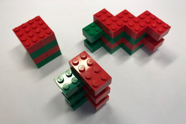
product looks like ‘putting boxes side by side’, for example:

                                                                         g
                        (g(f ⊗ 1)(|ψi ⊗ |φi)) ⊗ 1
                                                                     f

                                                                     ψ       φ

So far, things don’t look so different from quantum circuits. However, the key trick was to write
the maximally entangled state, and its adjoint, as bent pieces of wire:

                                := |00i + |11i                     := h00| + h11|                        (1)

    Then, the main idea behind quantum teleportation, which basically amounts to this equa-
tion:
                          ((h00| + h11|) ⊗ 1)(1 ⊗ (|00i + |11i)) = 1
becomes something visually very intuitive:

Hence, kindergarten quantum mechanics became a thing. Now, these sort of tricks weren’t
entirely new, as a certain Nobel Prize winner named Roger Penrose got so fed up in the 1970’s
with staring at indices in the tensor notation of relativity, and for that purpose invented exactly
the same kinds of pictures. So we were in pretty good company.
    A good start, but, how much mileage can you get out of these sort of tricks? Well, as it
turns out, a lot: one can teach an entire quantum computing and quantum foundations course
in these terms.1 How much is really new? That is, can drawing pictures of quantum processes
allow us to do things we couldn’t do before? Or is it just an art project?
    This is where the ZX-calculus comes in. The ZX-calculus is a graphical language for ex-
pressing quantum computations, mainly over qubits. While it’s been around since 2008, things
have only really started booming around 2018, with the appearance of several major results:
 (1) The ZX-calculus has been ‘completed’, which means all equations concerning quantum
     processes involving qubits that can be derived using linear algebra can also be obtained
     using a handful of graphical rules [68, 109]. This consolidates the promises made in the
     early days of kindergarten quantum mechanics, that graphical reasoning should not merely
     be seen as a helpful gadget, but as a genuine alternative to the Hilbert space formalism.
   1
    This course has been running since 2012 at the University of Oxford, and this course formed the basis for
‘dodo book’ [39]. https://www.cs.ox.ac.uk/teaching/courses/2019-2020/quantum/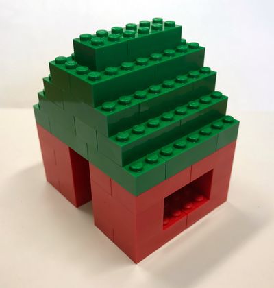
(2) For certain quantum circuit optimisation problems, ZX-based methods now outperform
the state of the art, e.g. [44] showed T-counts that were up to 50% better than known
techniques at the time of publication. These simplifications are important for making
the problems fit on existing quantum computers, and has played an important role in
the design of commercial quantum compilers such as Cambridge Quantum Computing’s
t|keti [103].
(3) ZX-calculus recently enabled a team to convert grammar-aware natural language process-
ing [42] into variational quantum circuits [27] suitable for running on existing, small-scale
quantum hardware, resulting in the first implementation of quantum natural language
processing on a quantum computer [86].
This paper is not intended to be a tutorial, but is an easy-going introduction and a survey of
some recent successes. If you are in need of a more detailed manual on how to use ZX-calculus,
several other resources are already available. For example, the book [39] gives an extensive
introduction to the broad subject of pictorial quantum reasoning, leading up to a detailed
presentation of ZX-calculus. While this is a pretty hefty tome (850 pages), it’s full of pictures
and has been taught multiple times (at Oxford, Nijmegen and Peking) in about 20 hours of
lecture time. A much shorter introductory ZX-tutorial is [31], and an extensive, up-to-date
introduction with many practical worked examples is [107]. There is moreover a forthcoming
secondary school book [37] that we discuss in Section 8.
2 ZX: LEGO for quantum computing
We will introduce ZX-calculus by comparing it to standard quantum circuit language, and in
particular, by explaining the manner in which ZX-calculus (quite literally) stretches beyond
how we can manipulate and reason with quantum circuits.
ZX-language. Typical primitives of quantum circuit language include the CNOT-gate and
certain single qubit gates like Z-phase gates and the Hadamard gate. We denote these here as
follows:
1 0 0 0
0 1 0 0 1 0 1 1 1
:= α := := √
0 0 0 1 0 eiα 2 1 −1
0 0 1 0
While Z-phase gates are typically taken to be diagonal in the standard (or ‘Z’) basis, we can
conjugate by the Hadamard gate to get X-phase gates, which are diagonal in the Hadamard
(or ‘X’) basis:
α := αThese two kinds of phase gates can now be used to build other things, for example, the
Hadamard gate itself now arises, up to a scalar factor (which we ignore), to it’s Euler de-
composition in terms of phase gates:
π
2
π
= 2
π
2
Rather than just using the standard phase gates as building blocks for other gates, ZX-
calculus uses generalisations thereof, allowing one to vary the number of incoming and outgoing
wires of these phase gates. More specifically, we can generalise the phase gates to ‘spiders’:
...
α := |0 . . . 0i h0 . . . 0| + eiα |1 . . . 1i h1 . . . 1|
...
(2)
...
α := |+ . . . +i h+ . . . +| + eiα |− . . . −i h− . . . −|
...
Without resorting to bra-ket notation, a Z-spider with m legs in and n legs out is a 2n × 2m
matrix with exactly 2 non-zero elements:
1 0 ··· 0 0
... 0 0
··· 0 0
:= ... ... .. .. ..
α
. . .
...
0 0 ··· 0 0
0 0 ··· 0 eiα
and an X-spider can be made from a Z-spider much like we did with phase gates:
... ...
α := α
... ...
Putting no α means α = 0, e.g.
1 0 ··· 0 0
... 0
0 ··· 0 0
:= ... .. . . .. ..
. . . .
...
0 0 ··· 0 0
0 0 ··· 0 1
It then follows that the cups and caps of (1), as well as many basic quantum states and effects,
are special cases of spiders:
= = = |0i π = |1i = |+i π = |−i
π π
= = = h0| = h1| = h+| = h−|√ √
where |+i = 1/ 2 |0i + |1i , |−i = 1/ 2 |0i − |1i , and we have ignored some normalisation
factors.
Spiders are all that the language of ZX-calculus consists of. Why can ZX-calculus get away
with only these? Since we can now build the CNOT-gate from these spiders as follows:
(3)
That this is indeed the case is something that can be easily checked using matrices. So in
particular, the CNOT-gate doesn’t have to be treated as a primitive anymore, but breaks down
in two smaller pieces. Once we have phase gates and the CNOT-gate, we know that we can
reproduce any quantum circuit made up of any gates.
What is the upshot of doing this? More specifically, why is this better than using standard
circuits? The true power of ZX-calculus arises from the fact that these smaller pieces in (3)
are very easy to work with, in the sense that the rules that govern them are easy to figure out,
remember, and do calculations with. Also, there aren’t many of them. In contrast, coming up
with all the rules that govern fixed sets of quantum gates is really hard, and little is known
beyond the case of very limited gate sets [2] or small fixed numbers of qubits.
For example, it was shown in [100] that there does exist a set of quantum circuit equations
rules that suffices to prove all true equations for 2-qubit circuits built from these gates:
π
4
That is, the gates we introduced at the beginning of this section, but with Z-phases restricted
to α = π/4. However, some of the rules are huge and difficult to work with. They can be found
in their entirity in [43], but to give a feel for their scale, here is the lefthand side of one of the
rules, which is too big to fit on the page:
π π −π
2
−π
4
π
4
π
4
−π
4
π
4
π
2
−π
4 ···
π
4
π
4
−π
4
π
4
π
2
−π
4
π π π
4
−π
2
−π
4 ···
(4)
··· π π π
4
−π
2
−π
4
π
4
−π
4
−π
4
π
4
π
2
··· π
4
−π
4
−π
4
π
4
π
2 π π −π
2
−π
4
We expect this situation to become worse as we go to more qubits. For example, it is hard
to imagine that a 3-qubit rule such as the following:
= (5)
could ever be proven using just the 2-qubit rules from [43, 100], or any 2-qubit rules for that
matter. Doing so seems to require decomposing at least one of the CNOT gates into single-qubit
gates, which is impossible. Of course, the devil is in the details, so we’ll leave the following as
a conjecture for now:Conjecture 2.1. No set of rules involving only two qubit circuits can be complete for circuits
with more than 2 qubits.
On the other hand, we’ll see in the completeness section 4 that it is possible to fit on one side
of A4 all the ZX-rules needed to prove all the equations that are true for for all ZX-pictures,
including circuits made from any gates with any number of qubits.
These much simpler ZX-rules reflect the fact that the ZX-language is in some way or another
more fundamental than circuits.
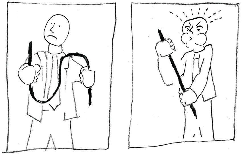
Consider an analogy using LEGO. The basic LEGO brick has been designed for it’s versatil-
ity, but if you were crazy enough to glue all of your LEGO together into some fixed ‘composite’
blocks, that famous versatility goes away. Just for fun, let’s take this a bit farther and suppose
there were indeed LEGO analogues for ZX-pictures:
ZX-language LEGO analogue
α α
γ
β
α
Standard LEGO allows for a wealth of creations:while the composite block only allows for a restricted spectrum of ‘art’:
In particular, circuit gates have unitarity imposed upon them, while the ZX-components have
been liberated from the unitary constraint.
If we want to actually run a computation on a quantum computer, it could be the case that
we only really care about unitary quantum circuits in the end. In that case, it is natural to
ask: is this extra freedom actually a good thing? We would contend that it is, and that we have
a situation that is somewhat analogous to complex analysis. In the case of complex analysis,
leaving real numbers behind (sometimes temporarily), gives us much more power and elegance,
even when proving things about real numbers. We will see this same phenomenon happening
for ZX-pictures in Section 5, where we discuss how to optimise quantum circuits by temporarily
leaving the circuit world, then coming back.
It was explained in [104] that the algebraic structures underlying the ZX-calculus are not
just normal LEGO, but ‘magic LEGO’, which are very bendy and enable all sorts of wild
creations. This is thanks to the flexibility of the graphical language, which we’ll discuss in the
next section. By only considering ‘glued-together’ LEGO, i.e. quantum gates, we miss out on
this whole story. So the moral is:
Stop gluing your LEGO together!
3 Basic ZX-rules
Spider fusion rules. Concretely, there are three kinds of rules governing the ZX spiders
(2). The first kind concerns how spiders of the same colour interact, and they are very simple:
spiders of the same colour ‘fuse’ together and their phases add up:
... ...
α ... α ...
... = ... = (6)
... α+β ... α+β
β
... β
...
... ...
One way to think of spiders is as ‘multi-wires’, in that while ordinary wires have two ends,
multi-wires can have multiple ends. The following multi-wires then happen to be ordinary
wires:
= = = = = =Now, what characterises a wire is that it connects its two ends, and if you connect two wires
together you again get a (now longer) wire. The same is true for multi-wires, and (6) just says
that if you connect two multi-wires, then you get another multi-wire.
There also is no real difference between a spider-input-leg and a spider-output-leg, as spider-
fusion allows these roles to be easily exchanged:
n
z }| { n+1
...
...
z }| {
... =
...
| {z }
| {z } m−1
m
More generally, this implies that in ZX-calculus:
only connectivity matters
and that we can think of ZX-pictures as graphs, that is, something that is specified by nodes
and edges connecting these. The loose legs then make it an ‘open’ graph [47]. This flexibility
is something that makes no sense for ordinary circuits, where each gate must have well-defined
inputs and outputs.
Strong complementarity rules. The second kind of rules concern the interaction between
spiders of different colours. They can either be stated as these two rules:
= = (7)
together with this third one:
= (8)
or, as this single rule:
... ...
= (9)
... ...
The rules (7) tell us that single leg spiders (a.k.a. states/effects), are copied by a spider of the
opposite colour. The rule (8) is slightly harder to interpret, and let’s not get us started about
(8). But they all follow a clear pattern, namely, the distinct colours can move trough each
other. Taking these rules, together with spider-fusion, one can derive this one [30]:
= (10)Let’s stress again that it is essential to have spider-fusion to derive this rule. Without it (9)
and (10) are independent. In fact, in mathematics, rule (9) defines a bialgebra, and having (10)
makes it a Hopf algebra (with trivial antipode) [22]. We will say something more about the
mathematical familiarity of these specific rules in Sec. 9.
Rule (10) has a very intuitive reading, namely, that two wires between spiders of opposite
colour always vanish. In other words, a 2-cycle always vanishes:
We can also give such an interpretation to (8), namely, that we can also eliminate all 4-cycles:
Rule (10) also has a very clear conceptual interpretation, namely, complementarity, or in
modern terminology, unbiasedness. One can show that spiders, when defined as linear maps
that obey spider-fusion are always uniquely fixed by a choice of orthonormal basis [41]. Then
(10) tells us that these two ONBs must be mutually unbiased [30,39]. Mutually unbiased bases
crop up all the time in quantum computing and quantum information theory. For example, a lot
of quantum cryptography, including the famous BB84 quantum key distribution protocol [11],
depends on mutually unbiased bases.
So the rule (10) defines pairs of mutually unbiased ONBs. Because, assuming spider-fusion,
the rule (9) is stronger than (10), we call is ‘strong complementarity’. A funny thing about
this novel notion of strong complementarity is that we actually know more about it then about
ordinary complementarity. We know that mutual strong complementarity is monogamous, so
it can only come in pairs [39, Thm. 9.66], and all of these pairs have been fully classified for
finite dimensional Hilbert spaces, in terms of the finite Abelian groups [32].
In terms of circuits, rule (10) tells us that CNOT-gates are unitary:
=
If instead of having the CNOT-gates acting on the same wire with the same colours, we do the
opposite, we get a circuit interpretation for (8):
=
Together these two circuit equations yield:
=A more extensive discussion of strong complementarity is in [39]. For now we stop discussing
rules, and do some stuff with the ones we have. We discuss rules further in the following section.
4 A complete calculus
Neither the rules (6) or (9) are specific to qubits, but make sense in all dimensions, and even
beyond Hilbert space quantum theory. Indeed, they provide a canvas for studying theories more
general than quantum theory, and they have for example enabled a crisp pictorial presentation
of Spekkens’ toy theory [7, 35, 36]. Notably, this kind of presentation enables one to pinpoint
exactly where quantum theory and interesting ‘quantum-like’ theories depart. In this case, it
has to do with the difference in the two finite groups Z4 and Z2 × Z2 . An extensive discussion
of all of this is in [39], Chapter 11.
Other papers on generalised theories based on strong complementarity include [32, 33, 59,
60, 63, 64]. All of this is part of the ‘process theories’ approach to quantum foundations, where
quantum-like theories are defined using a symmetric monoidal category, a.k.a. a process theory,
and their features are studied abstractly (see e.g. [25, 26, 61, 62, 74, 82, 92, 93, 98, 99]).
However, if we come back down to earth, we can look at which rules actually are specific to
quantum computation with qubits. As we will see, we don’t need to go too far before we have
enough rules to prove every true equation between pictures.
Qubit related rule(s). Turning our attention to Hilbert space again, and qubits specifically,
another rule that was part of the ZX-calculus early on, although in a very different form, is the
following one:
π π
2 2
-π
2
-π
2
= -π
2 (11)
-π
2
π
2
The form in which it appeared initially was the 1st one of these rules [29]:
... ... π
2
α
= α
= π
2 (12)
... ... π
2
which is a pretty one, with the 2nd one added a bit later [50], which is slightly less pretty.
Together these two rules involving the yellow box are equivalent to (11). So what is (11) telling
us?
We already told you about X spiders and Z spiders, but you might be wondering ‘what
happened to Y?’ Did we put our brains in the oven and cook our Y’s?
No! In fact, we didn’t define Y-spiders, because they can already be defined in two different
ways: in terms of an X-spider or in terms of a Z-spider. Equation (11) relates those two different
ways.
This rule comes from the geometry of the Bloch sphere, a common way to visualise qubit
operations as sphere rotations, in order to rotate X/Z into Y. Alternatively, you can slightlymodify this rule as follows:
-π
2
-π
2
-π
2
-π
2
= -π
2
π
2
π
2
which really is:
-π
2
-π
2
-π
2
-π
2
-π
2
-π
2
= =
π
2
π
2
π
2
And hence-ish the equivalence with rules (12). See [39] for a proper proof, without the ‘ish’. :)
A complete set of rules So what can we prove with the rules we now have? That is:
... ...
α ... α ...
... . . .
. . . = α+β . . . = α+β
β
... β
...
... ...
(13)
... ... π π
-π -π
2 2 2 2
= = -π
2
... ... -π
2
π
2
We already pointed out in Section 2 that with ZX-calculus we can go all the way and prove
every equation that one can prove using linear algebra. It was shown in shown in [96] that
these rules are not enough just yet.
However, Backens [3] showed that they do enable us to prove every equation that holds for
stabilizer quantum theory, i.e. ZX-pictures with phases restricted to multiples of π/2.
This is surely not an unimportant fragment of quantum theory, as, for example, it suffices
to prove that quantum theory is non-local [32]. On the other hand, stabiliser quantum circuits
can be efficiently simulated classically [65].
In practice, even though the ZX-rules above cannot prove all equations involving circuits
beyond stabiliser quantum theory, they seem pretty capable for many practical tasks such as
circuit optimisation, as we’ll see in the next section.
Of course, we do really want to understand which extra rules are needed in order to be able
to prove all equations. These were established for the first time by Ng and Wang in [87], buildingfurther on Hadzihasanovic’s result on a graphical calculus related to the ZX-calculus [67, 68].
Along the way, a result by Jeandel, Perdrix and Vilmart established derivability of all equations
for the ‘Clifford+T’ ZX-pictures, which generalise stabilisers by allowing multiples of π/4 rather
than only π/2 [71].
Theorems like these are called completeness theorems, in the sense that the rules form
a complete set with respect to derivability. There are now several different complete sets
of rules for the full family of ZX-pictures [87, 109], as well as the various different special
cases [71–73, 108]. The most succinct one currently around adds a single rule to the 4 rules
above, which allows for exchanging the colours of the phases in triples [109]:
γ γ̃
β = β̃ (14)
α α̃
where each of the phases α̃, β̃, γ̃ are trigonometric functions of the phases on the left-hand side.
This rule was first introduced for the case of two-qubit circuits [43], with two of the authors
of the present paper failing to realise that it would yield full-blown completeness as well. This
seems to show us that the four basic rules (13) already capture all of the complex interactions
of multiple qubits, up to some ‘local’ single qubit equations, which are all subsumed by (14).
So, if we have a complete set of rules for all ZX-pictures, we should be happy right? Wrong!
Completeness should be seen as the beginning and not the end for the ZX-calculus, and there
is much to be gained by finding better rules.
For example, the succinctness obtained from the introduction of the colour-exchanging rule
(14) comes at the price of introducing complicated, trigonometric functions of phases whenever
it is applied. In fact, these are ugly enough that we didn’t even bother to write them here. If we
are working with phases numerically on a computer, this isn’t a big problem, but for symbolic
manipulation this quickly becomes impractical.
One way around this problem is to shift to the algebraic ZX-calculus, which replaces the
phases α ∈ [0, 2π) – which become eiα in the definition of a spider (2) – with plain ol’ complex
numbers a ∈ C: ... ...
α a
... ...
Our previous notion of spiders are still around, just by setting a := eiα , but the extra generality
buys us several nice features such as a more direct encoding of complex-valued matrices as
well as straightforward generalisations from 2D to all finite dimensions [111] and from complex
numbers to any commutative semi-ring [110].
5 Automated circuit optimisation
If a circuit is given, can ZX-calculus help with simplifying it? Of course it can, and it seems to
be better at it than anything else. Here’s an example of how that works. Suppose we want to
simplify the following circuit made up of multiple gates, and we need to measure the last twoquibits:
measure these
z }| {
-π
4
π
4
π
4
-π
2
π
4
-π
4
| {z }
qubits prepared in |0i
There are a lot of 4-cycles here, and we’ve just learned that ZX-calculus is good at getting rid
of 4-cycles. The 4-cycles are here:
-π
4
π
4
-π
4
However, they are not 4-cycles because they happen to look like rectangles, as the 4-cycles we
are looking for has alternating colours as corners. We can do some (un-)fusing:
π
4 = π
4 = π
4
and now we can eliminate that square, and then re-arrange a bit:
π
π
4 = 4 =
π
4We can do the same for the other 4-cycles:
-π
4 = -π
4 =
-π
4
-π
4
What we get has been called a ‘phase gadget’ [77]. By using the trick for eliminating 4-cycles
again, one also finds that phase gadgets with opposite angles cancel out:
π
4
=
-π
4
Hey ho let’s go. We first bring in phase gadgets and then fuse:
-π
4
π
4
-π
4
π
4
-π
4
π
4
π
4
= π
4
= π
4
-π
2
-π
2
-π
2
π
4
-π
4
π
4
π
4
-π
4
-π
4
We get a 2-cycle which as we know vanishes, and then the two qubits on the left completely
disentangle from those on the right, so we can forget about them:
-π
4
π
4
π
4
π
4
=
-π
2
π
4
-π
4
-π
4
resulting in the fact that we end up with what we started with, despite the whole circuit looking
pretty complicated when we started.
While it is easy to work on small circuits by hand, we would also like to apply these
techniques to circuits with thousands or millions of quantum gates, so it is natural to considerFigure 1: PyZX is a Python library and circuit optimsation tool using the ZX-calculus. See
github.com/Quantomatic/pyzx.
how these kinds of simplifications can be automated. A standard method for this is to replace
equations, which can be applied in either direction, with directed rewrite rules. For example:
... ...
α ... α ...
... = ... → (15)
... α+β ... α+β
β
... β
...
... ...
As long as the rules decrease some metric of the ZX-picture (e.g. the number of spiders),
applying them blindly until they don’t apply any more will always terminate. In rewrite theory
lingo, this means we can automate simplification of ZX-pictures by using a terminating rewrite
system, based on a subset of the ZX-calculus rules.
This rewriting can be formalised in such a way that ZX-pictures can be represented and
transformed by software tools using a method called double-pushout graph rewriting [54]. The
basic theory for representing ZX-pictures as graphs and rewriting them was presented in [47],
and recently extended in [14]. This forms the basis of a diagrammatic ‘proof assistant’ called
Quantomatic [78].
By ‘breaking open’ the gates in a quantum circuit, we can find simplifications in the ZX-
calculus that would be hidden at the gate level. However, we may end up with something
that doesn’t look at all like a circuit any more. Hence, an important problem for ZX-based
optimisation techniques is circuit extraction, that is efficiently recovering a gate-decomposition
from a simplified ZX-picture. This simplify-and-extract technique for ZX was introduced in [49],
generalised to a broader family of diagrams in [6], and forms the basis of the quantum circuit
optimisation tool PyZX [76] (Fig. 1).
ZX-picture rewriting also forms the basis of a special-purpose circuit simplification tool
STOMP [44], which reduces an important cost metric called the T-count of a quantum circuit
using so-called ‘spider-nest’ identities.6 Quantum Natural Language Processing
ZX-calculus grew out of a more general pictorial approach to quantum foundations and quantum
computation, called categorical quantum mechanics (CQM) [1, 23]. In fact, what CQM does
is propose an alternative formalism to Hilbert space, which puts the emphasis on how systems
compose, rather than in which space systems are described. Thanks to the successes of ZX-
calculus it is fair to say the this alternative has genuine practical advantages.
On the other hand, the graphical structures employed by CQM (and in many cases orig-
inating there) stretch well beyond quantum theory. For example they have been applied in
computability theory [89], models of concurrency [105], control theory [9, 19], the study of elec-
trical [10] and digital [57] circuits, game theory [56], broader cognitive features [13], natural
language processing [42, 95], and even consciousness research [102, 106]!
As aspects of ZX-calculus are essential to some of these areas, one may argue that to some
extent they are ‘quantum-like’. While this may only be taken as a rough analogy in some
cases, in the particular area of natural language processing (NLP), it seems to be useful to take
this quantum connection seriously. In the approach to NLP put forward in [42], vector space
models for word meaning were combined with grammatical structure to produce compositional
models of sentence meaning. As this model makes crucial use of this tensor product of vector
spaces, which gives exponential space requirements on a classical computer. On the other hand,
forming tensor products on a quantum computer is cheap, as this is just what happens when
you put two pieces of quantum data next to each other. This realisation led to the proposal
of a quantum algorithm for natural language processing [113]. For various reasons, this first
proposal was not very practical to run on quantum computers of today or the near future.
More recently, this proposal was adjusted and refined in order to fit on currently existing
quantum hardware [27,85], and implemented on IBM’s quantum devices [86]. This provided an
example of a ‘quantum native’ solution to a classical problem. That is, while the problem has
nothing to do with quantum systems, it’s structure still naturally lives on a quantum computer.
An important refinement from the original algorithm to the one recently implemented on
a real quantum computer was the use of the ZX-calculus to turn a picture representing a
natural language sentence into a runnable quantum circuit that computes something about
the sentence’s meaning within the NLP model. Here is an example of a sentence and it’s
interpretation as a picture:
*hates*
Alice Bob
JAlice hates Bob.K =
To ‘run’ this sentence on a quantum computer, we first interpret the black dot as the green
ZX-spider. We can now use ZX-calculus to turn it into circuit-form:
*hates* Alice *hates* Bob
Alice Bob
=
We may then use ZX-calculus rules to massage this diagram into a different shape (who’smeaning is equivalent):
Alice Bob
Alice *hates* Bob
= *hates* (16)
and replace the word-meanings by some pieces of ZX-picture with free parameters, α, β, ...:
αA αp αB
Alice Bob
βA βB
α
β
hates
α0 + γ
β0
γ0
These parameters are ‘trained’ over the course of many runs of such circuits using machine
learning techniques. The finished product is a quantum circuit capable in principle of comparing
sentence meanings, answering questions, and doing many more linguistic tasks.
This very simple sentence only uses a dash of ZX-calculus, but it already becomes clear
that the ‘elasticity’ of ZX is helpful for such tasks. There are many equivalent ways to compute
the sentence meaning, and some fit better on a quantum computer than others, hence the
‘massaging’ in equation (16). This really starts to pay off when one starts to consider more
complex sentences like this one:
who who
Bob is silly loves Alice is rich
This can be seen as a compilation process, but one that doesn’t take a program language as
input, but natural language, and turns it into quantum machine code using the ZX-calculus to
handle everything in between. The end result is a physics-first: the use of quantum systems to
process natural language, with the help of the ZX-calculus.
Quantum machine learning plays a central role in quantum natural language processing.
Recently, the ZX-calculus has started to play a role in enhancing our understanding of quan-
tum machine learning itself: first in picturing quantum ansätze [112], and then in analysing
important problems within the approach like the barren plateu phenomenon [114].7 MBQC and Fault-tolerance
Measurement-based quantum computing (MBQC) is an alternative model of computation to the
circuit model, where measurements, rather than quantum gates, are the main things driving the
computation. The most well-studied MBQC setup is called the quantum one-way model [94]
In this setup, many qubits are prepared in a certain fixed state, called a graph state, then
single-qubit measurements are prepared in a particular order.
Notably, the choice of the kind of measurement performed can depend on past measurement
outcomes, a principle referred to as feed-forward. Even though each individual measurement
outcome is non-deterministic, a clever application of feed-forward can produce deterministic
quantum computations.
For example, in the one-way model, measurements are defined by angles α ∈ [0, 2π). When
they are performed, one of two things happens, non-deterministically:
α α+π
or .
Suppose we actually wanted the first outcome for our computation, then the ZX-calculus tells
us how to ‘push’ the unwanted π forward in time, changing future measurement angles:
feed-forward
γ
...
...
...
γ π γ+π
β
β π -β
= =
α+π
α α
π error
...
...
...
In fact, making these kinds of computations in the one-way model easier was one of the
original motivations for the ZX-calculus. ZX was used, for example, to teach the one-way model
in a fully-graphical way [39], give the first technique for translating MBQC computations into
circuits that didn’t require extra qubits or (non-physical) feedback loops [51], and produce an
alternative model for MBQC based on Pauli-ZZ interactions [75], which are the native 2-qubit
gate for most types of quantum hardware.
Another popular family of measurement-based models of quantum computation are vari-
ous forms of fault-tolerant computations based on the surface code, a type of quantum error
correcting code. Quantum error correction, and fault-tolerance is a huge subject, and way too
huge to cover here. However, the basic idea is that many low-level ‘physical’ qubits correspond
to a few ‘logical’ qubits. When doing computation in this way, it is useful to abstract away
individual operations on the physical qubit to and certain high-level logical transformations. A
particularly nice instance of this is lattice surgery [70], which was co-developed by one of the
authors of this survey. In lattice surgery, the main logical operations are ‘Z-split’, ‘X-split’,
‘Z-merge’, and ‘X-merge’. You might notice that I just said ‘ZX’ twice, so maybe this is a job
for the ZX-calculus!
Indeed, in [46], the authors showed that ZX is a natural language for lattice surgery com-
putations. For one thing, the basic operations are exactly what they sound like:split! split!
Z X
Z X
merge! merge!
Since these are just spiders, we already know how to use lattice surgery operations to build,
for example, a CNOT gate:
= (17)
While splits can be done deterministically, merges might introduce a π error. However, much
like in the one-way model, these errors can often be fed-forward using ZX-rules and accounted
for by later operations:
π error feed-forward
π
π
= =
π
This ZX language for lattice surgery was given a formal foundation in [45] and variations have
been used by groups at Google [58] and NII Toyko [69] for optimising various aspects of fault-
tolerant computations.
While originally envisioned as a model based on the new primitives of split and merge,
subsequent work has focused mainly on using lattice surgery as a tool for building CNOT gates
as in equation (17) (with a few notable exceptions, e.g. [83]). Interestingly, in 2020 we saw the
first experimental demonstration of logical qubit entanglement using lattice surgery [55, Nature],
where the authors noted that it was much more efficient to use the primitive split and merge
operations to prepare an entangled state. They did it like this:
= =
8 Kindergarten quantum mechanics: the experiment
In the abstract, we claimed that this paper is a spiritual child of the 2005 lecture notes Kinder-
garten Quantum Mechanics [23], but in fact, it is rather a spiritual grandchild. The middle
generation was a paper called Quantum Picturalism [24], which contained among other things a
vague proposal for testing the effectiveness of the pictorial formalism. It was claimed that, given
the proper learning materials, high-school students could outperform their teachers in quantum
theory, if the students used the pictorial formalism while the teachers used the Hilbert space
formalism.Now, ten years later, we have the materials in place for a far more ambitious goal: getting
high-school students to do state-of-the-art quantum computing, on par with the abilities of
Oxford post-graduate students. First of all, this required a book specifically targeted at high-
schoolers, and a set of tasks to set both the high-schoolers and the postgrads, and some other
interesting groups (like art students!). The book [37] and the tasks are written, but still under-
wraps until the experiment is done. Without giving too much away, this should give some idea
of the tone of the book:
The experiments have already begun. Watch this space!
9 How we got here: a brief history of the ZX-calculus
Conception. ZX-calculus was ‘born’ in a rejected conference abstract [28] (QIP 2007), writ-
ten in the mountains north of Tehran. The referee reports said things like:
‘Looks cute, so what?’
The basic idea at the time was to expand categorical quantum mechanics to complemen-
tary quantum observables, with the now-stated aim to make it directly applicable to practical
quantum computing, but the deeper goal was to do something the program of Birkhoff-von Neu-
mann quantum logic [12] failed to do: produce from first principles a full-fledged alternative
to Hilbert space quantum theory. Strong complementarity was reverse-engineered by looking
at ‘generalised flow’ for MBQC [51], and phases just followed from general abstract nonsense,
a.k.a. category theory.
ZX-calculus was ‘officially’ introduced in the accepted conference paper [29, ICALP, 2008].
A slightly unfortunate statement in [29] concerns the relative status of complementarity (10) and
strong complementarity (9): it was shown (in Theorem 3) that under a ‘mild assumption’ these
are equivalent. Later, in the 85 page corrected and substantially expanded journal version [30,
NJP, 2011] that ‘mild assumption’ was in Thm. 9.24 shown to be essentially equivalent to strong
complementarity. A proper treatment of the (huge!) difference between complementarity and
strong complementarity appeared in [32], by establishing a connection with non-locality, and
fully classifying strongly complementary bases. (The full classification of complementarity bases
is still completely open, and has swallowed several careers whole.)
Early rule fuzz. One of the early goals of the ZX-calculus was to fully understand MBQC
using pictures. In doing so, it quickly become clear that the Euler decomposition rule on the
right of equation (12) was needed in addition to rules that were already established [50]. This
than settled the core of ZX-calculus, as it still is now.
After that, we attempted to move ZX-calculus beyond bog-standard quantum gates and
MBQC to describe W-states. In quantum entanglement theory, there is ‘essentially’ only one
two-qubit entangled state, up to equivalence by so-called stochastic local operations, but for 3qubits there are two [53]. One is called a GHZ-state, and is just a 3-legged spider, and the
other is called a W-state.
At first, a lot of time and energy was spent trying to cram W-states into the ZX-calculus.
Along the way we got a useful new ZX-rule (supplementarity [34]), but we didn’t get much
closer to being able to work with W-states. This early defeat made some of us consider an
alternative to the ZX calculus which is now called the...
ZW-calculus. The completeness of ZX-calculus was initially proven using completeness of
another calculus: the ZW-calculus, a.k.a. the GHZ/W calculus [38]. The key idea was to
slightly vary the rules governing spiders as follows:
... ... ... ...
...
...
... = but ... =
... ...
...
...
... ... ... ...
These spiders were called W-spiders, as the W-state was an instance of them. While this seemed
like a relatively minor tweak to the notion of spiders, it turned out that, unlike the ZX-calculus,
it was relatively straightforward to find a complete set of rules [66], owing in part to the fact
that the ZW-calculus it more directly encodes the rules of arithmetic [40].
The first completeness theorems for the ZX-calculus were proven using a somewhat round-
about technique that encoded ZX-pictures as ZW-pictures and showed (painstakingly) that
each of the ZW-rules was derivable in ZX. This proved an important step in the progress of ZX
theory, but the original raison d’etre for ZW remains open:
Open problem. 9.1. Provide a classification of many-qubit entanglement (which is still poorly
understood beyond three qubits) using the ZW-calculus.
A dead end: the ‘XYZ-calculus’. An early variation on ZX-calculus was the trichromatic
calculus of [81], where a third colour (i.e. the Y-observable) was added. As one cannot have
the cups for all three observable coincide, for the sake of symmetry, none did. This resulted
in a substantially more complex rule-set and the calculus was never really used. The reason
it shouldn’t be used, probably, is because of monogamy of strong complementarity [39]. That
is, at most two colours of spiders can satisfy the strong complementarity rules described in
section 4 with each other, so to accommodate more colours, you have to put some sort of
‘awkward twist’.
(In)completeness and presentations. The rules of ZX-calculus as firstly introduced in [30]
without much consideration for scalar factors. These tended to be ignored when it was con-
venient, which causes problems e.g. for computing probabilities of quantum measurement
outcomes. Scalars were seriously considered in the rules for the stabilizer fragment of ZX-
calculus [5]. Minimality (whether a rule is non-derivable from other rules) of ZX rules was
initially considered in [8] for stabilizer ZX-calculus, then it was further investigated for Clif-
ford+T ZX-calculus in [101].
As mentioned in section 4, the first breakthrough for completeness of ZX-calculus was made
by Backens [3] for the stabilizer fragment. The completeness of the real stabilizer ZX-calculus
then followed in [52]. Furthermore, Backens proved that the scalar version of stabilizer ZX-
calculus and the single-qubit Clifford+T fragment of ZX are complete [4, 5]. At the sametime, Schröder de Witt and Zamdzhiev showed by a counter-example that ZX-calculus can’t be
universally complete if it is just equipped with stabiliser-style rules [97]. They also conjectured
that completeness could be achieved by adding a rule of form (14). Later on, Perdrix and
Wang proved that the stabiliser-style ZX even can’t be complete for the multi-qubit Clifford+T
fragment, and the supplementarity rule is necessary [91].
At some point, some people (including at least one of the authors of this paper) started
to believe there would be no finite set of rules which would be complete for any substantial
extension of stabiliser quantum theory.
Fortunately, the aforementioned author didn’t put money on it, as 2017-18 saw a veritable
frenzy of completeness results for ZX. First Jeandel, Perdrix, and Vilmart (a.k.a. ‘team Nancy’)
proved the completeness of multi-qubit Clifford+T ZX-calculus with a translation from ZW-
calculus [71]. Very soon after, Ng and Wang finished the first complete axiomatisation for
universal qubit ZX-calculus using a similar approach to the Nancy team and by introducing
some new generators to the theory [87]. They were also able to give a (different) complete
axiomatisation for the multi-qubit Clifford+T fragment [68, 88]. Inspired by Ng and Wang’s
results, the Nancy team gave another complete axiomatisation for universal qubit ZX-calculus
in terms of original ZX spiders [72]. Furthermore, they proposed a normal form for ZX diagrams
based on which universal completeness was still obtained without any resort to translation from
ZW-calculus [73]. At last, as we mentioned in section 4, Vilmart successfully proved Schröder
de Witt and Zamdzhiev’s conjecture with the explicit expression of (14) [109].
Precursors and successors. The kind of pictorial reasoning used in this paper was initiated
by Penrose as a more intuitive alternative for ordinary tensor notation [90]. In fact, even though
Penrose had reportedly been using the notation since he was an undergrad, he didn’t think too
highly of its prospects, mainly due to typesetting issues. In his 1984 text Spinors and Spacetime,
he notes:
The notation has been found very useful in practice as it greatly simplifies the
appearance of complicated tensor or spinor equations, the various interrelations
expressed being discernible at a glance. Unfortunately the notation seems to be
of value mainly for private calculations because it cannot be printed in the normal
way.
Of course a lot can change in 20 years. In 2004, this notation was adopted to the specific
needs of (finite-dimensional) quantum theory in CQM [1], which started the compositional
axiomatization of quantum theory.
Spiders, in their algebraic incarnation as certain Frobenius algebras, first appeared in the
category-theory literature [21,79]. Hopf algebras, which in ZX-calculus terms correspond to the
strong complementarity rules in absence of the spider-rules, have been around in their current
concrete form since 1956 [22], when Cartier generalised earlier definitions based on structure
theorems on the cohomology of compact Lie groups by Hopf, Samelson, Borel and others in the
1940s. Hopf algebras and their representations are now studied extensively under of moniker
of quantum group theory (see e.g. [84]).
The idea of depicted (classical boolean) circuits as pictures of more basic components, and
the pictorial depiction of the Hopf algebra (a.k.a. strong complementarity) laws, goes back to
Lafont [80]. However, to capture the full richness of quantum circuits, one needs not just a single
Hopf algebra, but a pair of them which interact in a special way (namely via the Frobenius,a.k.a. spider fusion laws). This structure was first made explicit, to the best of our knowledge,
as part of the ZX-calculus.
Notably, this structure contains non-trivial algebraic parts (i.e. those with operations taking
many inputs) and non-trivial co-algebraic parts (i.e. those with operations producing multiple
outputs), which interact with each other. This novel mathematical structure is interesting in its
own right, and has since been studied using category theory [16,18,20,48] and found a multitude
of applications e.g. in the study of signal-flow graphs [17] and concurrent systems [15].
The future. New papers on ZX-calculus are appearing at a steadily increasing rate, and
we can only expect that increase to continue. There is a regularly updated list of papers on
ZX-calculus available here that you may want to consult in the future:
https://zxcalculus.com/publications.html
References
[1] S. Abramsky and B. Coecke. A categorical semantics of quantum protocols. In Proceedings
of the 19th Annual IEEE Symposium on Logic in Computer Science (LICS), pages 415–
425, 2004. arXiv:quant-ph/0402130.
[2] M. Amy, J. Chen, and N. J. Ross. A finite presentation of cnot-dihedral operators. In
Bob Coecke and Aleks Kissinger, editors, Proceedings 14th International Conference on
Quantum Physics and Logic, Nijmegen, The Netherlands, 3-7 July 2017, volume 266 of
Electronic Proceedings in Theoretical Computer Science, pages 84–97. Open Publishing
Association, 2018.
[3] M. Backens. The ZX-calculus is complete for stabilizer quantum mechanics. New Journal
of Physics, 16:093021, 2014. arXiv:1307.7025.
[4] M. Backens. The ZX-calculus is complete for the single-qubit Clifford+T group. In B. Co-
ecke, I. Hasuo, and P. Panangaden, editors, Proceedings of the 11th workshop on Quantum
Physics and Logic, volume 172 of Electronic Proceedings in Theoretical Computer Science,
pages 293–303. Open Publishing Association, 2014.
[5] M. Backens. Making the stabilizer ZX-calculus complete for scalars. Electronic Proceedings
in Theoretical Computer Science, 195:17–32, November 2015.
[6] M. Backens, H. Miller-Bakewell, G. de Felice, and J. van de Wetering. There and back
again: A circuit extraction tale. arXiv preprint arXiv:2003.01664, 2020.
[7] M. Backens and A. Nabi Duman. A complete graphical calculus for Spekkens’ toy bit
theory. Foundations of Physics, 2015. arXiv:1411.1618.
[8] M. Backens, S. Perdrix, and Q. Wang. Towards a Minimal Stabilizer ZX-calculus. Logical
Methods in Computer Science, Volume 16, Issue 4, December 2020. arXiv:1709.08903.
[9] J. C. Baez and J. Erbele. Categories in control, 2014. arXiv:1405.6881.
[10] J. C. Baez and B. Fong. A compositional framework for passive linear networks.
arXiv:1504.05625, 2015.[11] C. H. Bennett and G. Brassard. Quantum cryptography: Public key distribution and
coin tossing. In Proceedings of IEEE International Conference on Computers, Systems
and Signal Processing, pages 175–179. IEEE, 1984.
[12] G. Birkhoff and J. von Neumann. The logic of quantum mechanics. Annals of Mathe-
matics, 37:823–843, 1936.
[13] J. Bolt, B. Coecke, F. Genovese, M. Lewis, D. Marsden, and R. Piedeleu. Interacting
conceptual spaces I. In M. Kaipainen, A. Hautamäki, P. Gärdenfors, and F. Zenker, edi-
tors, Concepts and their Applications, Synthese Library, Studies in Epistemology, Logic,
Methodology, and Philosophy of Science. Springer, 2018. to appear.
[14] F. Bonchi, F. Gadducci, A. Kissinger, P. Sobocinski, and F. Zanasi. String diagram
rewrite theory i: Rewriting with frobenius structure. arXiv preprint arXiv:2012.01847,
2020.
[15] F. Bonchi, J. Holland, R. Piedeleu, P. Sobociński, and F. Zanasi. Diagrammatic algebra:
from linear to concurrent systems. Proceedings of the ACM on Programming Languages,
3(POPL):1–28, 2019.
[16] F. Bonchi, R. Piedeleu, P. Sobociński, and F. Zanasi. Graphical affine algebra. In 2019
34th Annual ACM/IEEE Symposium on Logic in Computer Science (LICS), pages 1–12.
IEEE, 2019.
[17] F. Bonchi, R. Piedeleu, P. Sobociński, and F. Zanasi. Contextual equivalence for sig-
nal flow graphs. In Jean Goubault-Larrecq and Barbara König, editors, Foundations of
Software Science and Computation Structures, pages 77–96, Cham, 2020. Springer Inter-
national Publishing.
[18] F. Bonchi, P. Sobocinski, and F. Zanasi. Interacting bialgebras are Frobenius. In 17th
International Conference on Foundations of Software Science and Computation Structures
(FOSSACS), pages 351–365, 2014.
[19] F Bonchi, P. Sobociński, and F. Zanasi. Full abstraction for signal flow graphs. In
Principles of Programming Languages, POPL‘15., 2015.
[20] F. Bonchi, P. Sobociński, and F. Zanasi. Interacting hopf algebras. Journal of Pure and
Applied Algebra, 221(1):144–184, 2017.
[21] A. Carboni and R. F. C. Walters. Cartesian bicategories I. Journal of Pure and Applied
Algebra, 49:11–32, 1987.
[22] P. Cartier. A primer of Hopf algebras. In Frontiers in number theory, physics, and
geometry II, pages 537–615. Springer, 2007.
[23] B. Coecke. Kindergarten quantum mechanics. In A. Khrennikov, editor, Quantum Theory:
Reconsiderations of the Foundations III, pages 81–98. AIP Press, 2005. arXiv:quant-
ph/0510032.
[24] B. Coecke. Quantum picturalism. Contemporary Physics, 51:59–83, 2009.
arXiv:0908.1787.[25] B. Coecke. A universe of processes and some of its guises. In H. Halvorson, editor, Deep
Beauty: Understanding the Quantum World through Mathematical Innovation, pages 129–
186. Cambridge University Press, 2011. arXiv:1009.3786.
[26] B. Coecke. Terminality implies no-signalling... and much more than that. New Generation
Computing, 34:69–85, 2016.
[27] B. Coecke, G. de Felice, K. Meichanetzidis, and A. Toumi. Foundations for near-term
quantum natural language processing. arXiv preprint arXiv:2012.03755, 2020.
[28] B. Coecke and R. Duncan. A graphical calculus for quantum observables. zxcalcu-
lus.com/publications.html, 2007.
[29] B. Coecke and R. Duncan. Interacting quantum observables. In Proceedings of the 37th
International Colloquium on Automata, Languages and Programming (ICALP), Lecture
Notes in Computer Science, 2008.
[30] B. Coecke and R. Duncan. Interacting quantum observables: categorical algebra and
diagrammatics. New Journal of Physics, 13:043016, 2011. arXiv:quant-ph/09064725.
[31] B. Coecke and R. Duncan. Tutorial: Graphical calculus for quantum circuits. In Inter-
national Workshop on Reversible Computation, pages 1–13. Springer, 2012.
[32] B. Coecke, R. Duncan, A. Kissinger, and Q. Wang. Strong complementarity and non-
locality in categorical quantum mechanics. In Proceedings of the 27th Annual IEEE
Symposium on Logic in Computer Science (LICS), 2012. arXiv:1203.4988.
[33] B. Coecke, R. Duncan, A. Kissinger, and Q. Wang. Generalised compositional theories
and diagrammatic reasoning. In G. Chiribella and R. W. Spekkens, editors, Quantum
Theory: Informational Foundations and Foils, Fundamental Theories of Physics. Springer,
2016. arXiv:1203.4988.
[34] B. Coecke and B. Edwards. Three qubit entanglement within graphical Z/X-calculus.
Electronic Proceedings in Theoretical Computer Science, 52:22–33, 2010.
[35] B. Coecke and B. Edwards. Toy quantum categories. Electronic Notes in Theoretical
Computer Science, 270(1):29 – 40, 2011. arXiv:0808.1037.
[36] B. Coecke, B. Edwards, and R. W. Spekkens. Phase groups and the origin of non-
locality for qubits. Electronic Notes in Theoretical Computer Science, 270(2):15–36, 2011.
arXiv:1003.5005.
[37] B. Coecke and S. Gogioso. Quantum theory in pictures, 2020. Tutorial.
[38] B. Coecke and A. Kissinger. The compositional structure of multipartite quantum entan-
glement. In Automata, Languages and Programming, Lecture Notes in Computer Science,
pages 297–308. Springer, 2010. arXiv:1002.2540.
[39] B. Coecke and A. Kissinger. Picturing Quantum Processes. A First Course in Quantum
Theory and Diagrammatic Reasoning. Cambridge University Press, 2017.
[40] B. Coecke, A. Kissinger, A. Merry, and S. Roy. The GHZ/W-calculus contains rational
arithmetic. Electronic Proceedings in Theoretical Computer Science, 52:34–48, 2010.[41] B. Coecke, D. Pavlović, and J. Vicary. A new description of orthogonal bases. Math-
ematical Structures in Computer Science, to appear, 23:555–567, 2013. arXiv:quant-
ph/0810.1037.
[42] B. Coecke, M. Sadrzadeh, and S. Clark. Mathematical foundations for a compositional
distributional model of meaning. In J. van Benthem, M. Moortgat, and W. Buszkowski,
editors, A Festschrift for Jim Lambek, volume 36 of Linguistic Analysis, pages 345–384.
2010. arxiv:1003.4394.
[43] B. Coecke and Q. Wang. ZX-rules for 2-qubit Clifford+T quantum circuits. In Jarkko Kari
and Irek Ulidowski, editors, Reversible Computation - 10th International Conference, RC
2018, Leicester, UK, September 12-14, 2018, Proceedings, volume 11106 of Lecture Notes
in Computer Science, pages 144–161. Springer, 2018.
[44] N. de Beaudrap, X. Bian, and Q. Wang. Fast and effective techniques for t-count reduction
via spider nest identities. In 15th Conference on the Theory of Quantum Computation,
Communication and Cryptography (TQC 2020). Schloss Dagstuhl-Leibniz-Zentrum für
Informatik, 2020. arXiv:2004.05164.
[45] N. de Beaudrap, R. Duncan, D. Horsman, and S. Perdrix. Pauli fusion: a computational
model to realise quantum transformations from ZX terms. In Bob Coecke and Matthew
Leifer, editors, Proceedings 16th International Conference on Quantum Physics and Logic,
Chapman University, Orange, CA, USA., 10-14 June 2019, volume 318 of Electronic
Proceedings in Theoretical Computer Science, pages 85–105. Open Publishing Association,
2020.
[46] N. de Beaudrap and D. Horsman. The ZX calculus is a language for surface code lattice
surgery. Quantum, 4:218, January 2020.
[47] L. Dixon and A. Kissinger. Open-graphs and monoidal theories. Mathematical Structures
in Computer Science, 23(02):308–359, 2013.
[48] R. Duncan and K. Dunne. Interacting frobenius algebras are hopf. In Proceedings
of the 31st Annual IEEE Symposium on Logic in Computer Science (LICS), 2016.
arXiv:1601.04964.
[49] R. Duncan, A. Kissinger, S. Perdrix, and J. Van De Wetering. Graph-theoretic simplifi-
cation of quantum circuits with the ZX-calculus. Quantum, 4:279, 2020.
[50] R. Duncan and S. Perdrix. Graph states and the necessity of euler decomposition. In
Conference on Computability in Europe, pages 167–177. Springer, 2009.
[51] R. Duncan and S. Perdrix. Rewriting measurement-based quantum computations with
generalised flow. In Proceedings of ICALP, Lecture Notes in Computer Science, pages
285–296. Springer, 2010.
[52] R. Duncan and S. Perdrix. Pivoting makes the ZX-calculus complete for real stabilizers.
In Proceedings of the 10th International Workshop on Quantum Physics and Logic, 2013.
arXiv:1307.7048.
[53] W. Dür, G. Vidal, and J. I. Cirac. Three qubits can be entangled in two inequivalent
ways. Physical Review A, 62(062314), 2000.You can also read