Molecular Ecological Network Complexity Drives Stand Resilience of Soil Bacteria to Mining Disturbances among Typical Damaged Ecosystems in China ...
←
→
Page content transcription
If your browser does not render page correctly, please read the page content below
microorganisms
Article
Molecular Ecological Network Complexity
Drives Stand Resilience of Soil Bacteria to
Mining Disturbances among Typical Damaged
Ecosystems in China
Jing Ma 1 , Yongqiang Lu 2 , Fu Chen 1,2, * , Xiaoxiao Li 2 , Dong Xiao 3 and Hui Wang 2
 1   Low Carbon Energy Institute, China University of Mining and Technology, Xuzhou 221008, China;
     jingma2013@cumt.edu.cn
 2   School of Environmental Science and Spatial Informatics, China University of Mining and Technology,
     Xuzhou 221116, China; TS18160128P31@cumt.edu.cn (Y.L.); lixiaoxiao@cumt.edu.cn (X.L.);
     wanghuei@cumt.edu.cn (H.W.)
 3   State Key Laboratory of Coal Resources and Safe Mining, China University of Mining and Technology,
     Xuzhou 221116, China; xd@cumt.edu.cn
 *   Correspondence: chenfu@cumt.edu.cn; Tel.: +86-0516-8388-3501

 Received: 16 February 2020; Accepted: 18 March 2020; Published: 19 March 2020

 Abstract: Understanding the interactions of soil microbial species and how they responded to
 disturbances are essential to ecological restoration and resilience in the semihumid and semiarid
 damaged mining areas. Information on this, however, remains unobvious and deficiently
 comprehended. In this study, based on the high throughput sequence and molecular ecology
 network analysis, we have investigated the bacterial distribution in disturbed mining areas across
 three provinces in China, and constructed molecular ecological networks to reveal the interactions of
 soil bacterial communities in diverse locations. Bacterial community diversity and composition were
 classified measurably between semihumid and semiarid damaged mining sites. Additionally, we
 distinguished key microbial populations across these mining areas, which belonged to Proteobacteria,
 Acidobacteria, Actinobacteria, and Chloroflexi. Moreover, the network modules were significantly
 associated with some environmental factors (e.g., annual average temperature, electrical conductivity
 value, and available phosphorus value). The study showed that network interactions were completely
 different across the different mining areas. The keystone species in different mining areas suggested
 that selected microbial communities, through natural successional processes, were able to resist the
 corresponding environment. Moreover, the results of trait-based module significances showed that
 several environmental factors were significantly correlated with some keystone species, such as
 OTU_8126 (Acidobacteria), OTU_8175 (Burkholderiales), and OTU_129 (Chloroflexi). Our study also
 implied that the complex network of microbial interaction might drive the stand resilience of soil
 bacteria in the semihumid and semiarid disturbed mining areas.

 Keywords: disturbed mining areas; soil microbial community; microbial network interactions;
 network topology; keystone taxa; soil resilience

1. Introduction
     Coal mining activities have resulted in surface subsidence, and have made the ecological
environment more fragile by creating huge, overburdening dumps and voids [1]. Recently, increasing
attention has been paid to the influences of coal-mining subsidence on the ecological environment [2].
The soil problems caused by coal mining have become increasingly prominent and already have been

Microorganisms 2020, 8, 433; doi:10.3390/microorganisms8030433          www.mdpi.com/journal/microorganisms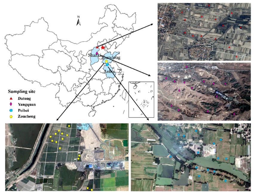
Microorganisms 2020, 8, 433                                                                         2 of 22

an important research topic in mining environmental ecology. Mining activities severely disrupt land
soils, resulting in the deterioration of the existing local ecosystems, such as destroying or degenerating
essential properties in the original soils [3]. The physical and chemical properties of existing soil and
microbial community characteristics have been seriously disturbed, and the quality of reclaimed or
restored soil has been quite poor [4]. Due to the protection of cultivated land and food security, the
ecological restoration of mining areas with high groundwater levels has focused on soil reclamation in
Eastern China. In the northern-western part of China, rapid and effective ecological restoration is also
in critical demand in order to ensure the sufficient management of semiarid, damaged mines.
      Using soil microbes is important in order to stimulate an ecosystem’s resilience. Assessment of the
diversity and activity of the soil microbial community is essential to evaluate the success of reclamation
or restoration. However, few studies have been conducted on the soil microbial community diversity
where there is a high groundwater level, or in semiarid damaged mining areas [5–7]. In this study, we
identified the dominant bacteria, which was critical to enhance our understanding, and determined
the ecological attributes of soil bacterial communities, which are abundant and ubiquitous in the soil
at different mining areas. Understanding the ecological attributes of dominant bacteria will increase
our capacity to successfully cultivate them, which is critical to successful restoration and reclamation
progress in mining areas [8,9]. In addition, understanding how soil bacterial communities vary across
space and how they respond to mining activities is also important for restoration ecology [10]. For
example, by locating and identifying some dominant taxa, which tend to prefer special environmental
conditions, such as mine cracks and surface subsidence, we can forecast their distribution and enrich
them to enhance the ecological restoration capacity of damaged mines. Thus, a better understanding
of dominant soil microbial taxa in the mining areas would improve our ability to manage soil bacterial
communities and promote their functional abilities.
      Microbial biodiversity includes the number of species, their abundance, and the complex
interactions among different species [11]. In the environmental habitats, massive microbial species
interact with each other to form complex ecological networks [12]. It is important to understand
microbial structural and functional effects, and the changes in microbial biodiversity, which might
be elucidated through the networks of interacting species. Additionally, it is essential, in studying
microbial biodiversity, to elaborate on and analyze the interactive network structures, as well as to
understand the underlying mechanisms. Therefore, in microbial ecology, the ecological networks of
biological communities have gained attention. However, it is still difficult to determine the network
structures and their relationships with environmental changes in microbial communities [13]. The
microbial community assembly process significantly affects the structure of microbial community, and
the selection process acts as one of the ecological processes controlling the assembly of the microbial
community. Moreover, this microbial interaction, which can be seen as a kind of selection, provides
some contributions to the microbial community assembly process [14]. Therefore, researchers have
increasingly studied microbial networks in diverse environments [15]. These microbial interactions
have been emphasized as being crucial to our understanding of the dynamics of microbial community
assembly alongside climate change [16]. Although some studies have investigated the changing
microbial interactions in response to different environmental disturbances, few studies have revealed
how microbial interactions vary in subsidence areas or damaged mines, especially in different locations.
Furthermore, deficiencies exist in how coal-mining activities have changed the structure of soil bacterial
communities and their interactions. Fortunately, in recent years, numerous studies have verified the
effect of land reclamation on soil bacterial communities after coal-mining disturbances [17]. Moreover,
some studies have focused on the relationship between changes in soil bacterial communities and
surrounding environmental factors. They discovered that changes in soil bacterial communities were
closely associated with soil properties, enzyme activities, and various types of vegetation cover. Some
studies also reported on how the structure of soil bacterial communities and their diversity changed
after coal-mining disturbances [7,17,18].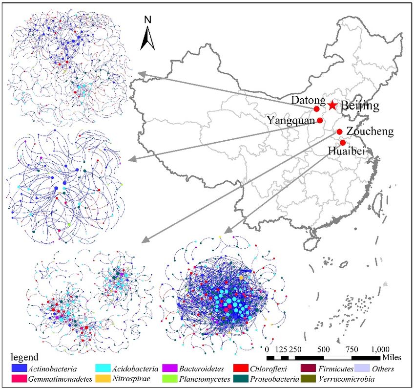
Microorganisms 2020, 8, 433                                                                            3 of 22

     The interactions of different microbial populations in a community play critical roles in determining
the functioning of an ecosystem, but little is known about the network interactions in the microbial
community, primarily because of the lack of appropriate experimental data and computational analytic
tools [19]. In recent years, high-throughput metagenomics technologies have rapidly produced a
massive amount of data, but one of the greatest difficulties in managing these data is deciding how
to extract, analyze, synthesize, and transform such a vast amount of information into biological
knowledge [20]. This study provided a novel conceptual framework to identify microbial interactions
and key populations based on high-throughput metagenomics sequencing data. The availability of
massive, community-wide, and replicated meta-genomic data from different mining areas has provided
an unprecedented opportunity to analyze network interactions in a microbial community [21].
     By combining massive data, we introduced molecular ecological network (MEN) construction
methods and the statistical analysis of bioinformatics to explore the controlling factors affecting the
distribution of microbial communities with high groundwater levels and in semiarid mining areas.
Furthermore, we explained the relationships between soil microbial communities and explored some
microbial keystone groups that could respond to and adapt to environmental changes. On the other
side, the network approaches might provide a new way to improve the ecological diversity and
ecosystem services in subsided or reclaimed mining areas, through a better decision-making, based
on a more complete evaluation. The appearance of molecular biological techniques provides new
methodologies to construct large-scale replicated networks, although system-level responses to change
remain mostly unexplored. We addressed three hypotheses in the current study: First, network
properties differed significantly among mining habitats on a large scale geographic scale level. Second,
the soil properties that correlated with keystone bacterial communities were different across the mining
areas. Third, the microbial distribution patterns across spatial distance, and the interactions of bacterial
communities among mining areas might drive different soil resilience levels in future mine restoration
and reclamation. Finally, we hope this study will aid in defining the recovery resilience of a damaged
mine ecosystem from the perspective of a microbial MEN, and revealed the development pattern of
microbiome, and the ecological restoration elastic enhancement mechanism.

2. Materials and Methods

2.1. Study Sites, Soil Sampling, and Measurment
      The Peibei (PB) coal-mining area (34◦ 130 39”N–34◦ 260 16”N, 117◦ 060 21”E–117◦ 120 16”E) is located
in Northern Anhui and Jiangsu Province (Figure 1). The study area has a warm temperate zone with a
semihumid monsoon climate and four distinctive seasons. The area has an annual average temperature
(AAT) of 14 ◦ C and an annual average precipitation (AAP) of 800–930 mm, which is a representative
semihumid area in East China. The soil type was haplic brown, and the sampling sites were in
the subsided mining areas. The Zoucheng (ZC) coal-mining area is located in Shandong Province
(35◦ 80 12”N–35◦ 320 54”N, 116◦ 460 30”E–117◦ 280 54”E), which is situated in a warm temperate monsoon
climate zone (Figure 1). This Geographically representative semihumid area of Eastern China has an
annual rainfall of 777.1 mm, and an annual average temperature of 14.1 ◦ C. The soil type is fluvo-aquic
soil. The samples were collected from the reclaimed farmland in the mining area. The Yangquan (YQ)
coal-mining area (113◦ 150 E–113◦ 180 E, 38◦ 010 N–38◦ 030 N) is located in Shanxi Province, China (Figure 1).
It has a continental climate, with an annual average temperature of 8.7 ◦ C, and an annual rainfall
between 450 and 550 mm, which is classified as a representative semiarid area of typical geographical
environment in Western China. The region is at the southern end of the Loess Plateau, and the main soil
type is calcareous cinnamon soil. Moreover, the ecological environment has been seriously damaged,
with frequent land cracks and an exposed vegetation root system along the surface. We collected the
soil samples from the damaged areas. The Datong (DT) coal-mining area (39◦ 530 24”N–40◦ 100 00”N,
112◦ 520 13”E–113◦ 320 35”E) is also located in Shanxi Province, China (Figure 1). This area used as the
representative semiarid area in Northern-Western China, has a continental climate and a mean annual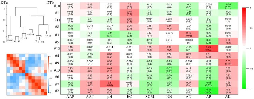
From June to August 2018, we collected approximately 500 g of surface (0–10 cm) soil from 14
discrete locations in the each mining area (Figure 1). We stored about 20 g of soil at −20 °C for
subsequent analysis of the microbial diversity. The remaining soil was air-dried and homogenized to
pass through a 2 mm sieve. We measured the soil pH and electrical conductivity (EC) values using a
pHMicroorganisms
     meter and2020,
                 a conductivity
                    8, 433         meter, respectively (PHC-3C, DDS-307A, Shanghai leici, China).    4 of 22We
measured the soil organic matter (SOM) according to colorimetrical methods using hydration heat
during the oxidation     of potassium dichromate. We also analyzed soil ammonium nitrogen (AN)
   temperature of 6.4 ◦ C. The mean annual precipitation is 384.6 mm, with precipitation mainly occurring
using the potassium chloride-ultraviolet spectrophotometry method, and measured the nitrate-
   from June to September. The collected soil type is loess and from the damaged mining areas. Using the
nitrogen
   diamond (NN)   content
              sampling       by calcium
                        method,   each soil chloride-ultraviolet
                                            sample was composedspectrophotometry.        We measured
                                                                    by 4 soil samples collected from plotsthe
available  phosphorus
   those were            (AP)
               9 m2 in size     using
                            in the fourthe hydrochloric
                                        mining  areas.   acid ammonium chloride method. We analyzed
the available soil potassium (AK) by the ammonium acetate–flame photometric method.

                                         Figure 1. Location of the study area.
                                        Figure 1. Location of the study area.
        From June to August 2018, we collected approximately 500 g of surface (0–10 cm) soil from
2.2.14DNA  Extraction,
       discrete        PCR
                locations    Amplification,
                          in the each miningand Illumina
                                              area        MiSeq
                                                    (Figure      Sequencing
                                                            1). We stored about 20 g of soil at −20 ◦ C for
   subsequent
     According analysis
                  to theofmanufacturer’s
                           the microbial diversity.  The remaining
                                            instructions,           soil was
                                                           we extracted   DNAair-dried
                                                                                 from and   homogenized
                                                                                       56 soil            to
                                                                                                samples taken
   pass through a 2 mm sieve. We measured the soil pH and electrical conductivity (EC) values using
from 0.5 g of fresh soil samples using the FastDNATM SPIN Kit for Soil (MP Biomedicals, Solon, OH,
   a pH meter and a conductivity meter, respectively (PHC-3C, DDS-307A, Shanghai leici, China). We
USA). We amplified the V4–V5 region of the bacterial 16S rRNA genes using the primer sets 515F (5′-
   measured the soil organic matter (SOM) according to colorimetrical methods using hydration heat
GTGCCAGCMGCCGCGGTAA-3′) and 907R (CCGTCAATTCMTTTRAGTTT). The DNA Gel
   during the oxidation of potassium dichromate. We also analyzed soil ammonium nitrogen (AN) using
Extraction Kit (Axygen Biosciences, Union City, CA, USA) was used to pool and purify the
   the potassium chloride-ultraviolet spectrophotometry method, and measured the nitrate-nitrogen (NN)
polymerase    chain reaction (PCR) products. We quantified the purified PCR products using the
   content by calcium chloride-ultraviolet spectrophotometry. We measured the available phosphorus
Quant-iT  PicoGreen    dsDNA acid
   (AP) using the hydrochloric  Assay  Kit (Invitrogen,
                                    ammonium      chlorideCarlsbad, CA,
                                                           method. We    USA). The
                                                                      analyzed       purifiedsoil
                                                                                 the available amplicons  were
                                                                                                  potassium
paired-end   sequenced
   (AK) by the  ammonium  (2 acetate–flame
                             × 300) on thephotometric
                                              Illumina MiSeq    platform using the MiSeq Reagent Kit V3
                                                          method.
(Personalbio, Shanghai, China). We distinguished the sample sequencing data according to the
   2.2. DNA
barcode        Extraction,
           sequence   andPCR     Amplification,
                            checked              and Illumina
                                       the sequence      of eachMiSeq  Sequencing
                                                                   sample   for quality control. Then we removed
the nonspecific         amplification
         According to the    manufacturer’s  sequences
                                                 instructions,and     chimericDNA
                                                                 we extracted      with     USEARCH
                                                                                      from 56  soil samples(v5.2.236,
                                                                                                              taken
http://www.drive5.com/usearch/)           in QIIME      (v1.8.0, http://qiime.org/).  We  clustered
   from 0.5 g of fresh soil samples using the FastDNATM SPIN Kit for Soil (MP Biomedicals, Solon,     the operational
taxonomic
   OH, USA).  units
                 We(OTUs)
                     amplifiedwith
                                 thea V4–V5
                                      97% similarity
                                               region ofcutoff    using the
                                                           the bacterial  16SUCLUST
                                                                              rRNA genesmethod
                                                                                            usinginthe
                                                                                                    QIIME    andsets
                                                                                                        primer    used
the515F     0
    Greengenes      database   (release  13.8,        0
                                                http://greengenes.secondgenome.com/)
          (5 -GTGCCAGCMGCCGCGGTAA-3 ) and 907R (CCGTCAATTCMTTTRAGTTT). The DNA                to  classify the species
[22,23]. We conducted
   Gel Extraction           alpha diversity
                     Kit (Axygen                indices
                                     Biosciences,    Unionto City,
                                                             revealCA,
                                                                     theUSA)
                                                                          richness,
                                                                                was diversity,
                                                                                    used to poolandand
                                                                                                     evenness    of the
                                                                                                         purify the
OTUs    and performed
   polymerase              beta diversity
                  chain reaction             analysis online
                                   (PCR) products.                using thethe
                                                          We quantified      open-source
                                                                               purified PCRplatform
                                                                                              products Metagenomics
                                                                                                          using the
forQuant-iT    PicoGreen Microbiology
     Environmental         dsDNA Assay Kit      (Invitrogen,http://mem.rcees.ac.cn:8080/).
                                             (DengLab;         Carlsbad, CA, USA). The purified    amplicons were
                                                                                                 According     to the
   paired-end    sequenced    (2 ×
taxonomic results, we constructed an abundance diagram and obtained rich infrared imagesV3
                                    300) on  the   Illumina   MiSeq   platform  using  the MiSeq   Reagent   Kit  with
   (Personalbio,
Origin             Shanghai,Northampton,
         9.1 (OriginLab,      China). We distinguished
                                                MA, USA)the   andsample  sequencing
                                                                    R software       data according to the barcodeThe
                                                                                 (https://www.r-project.org/).
   sequence and checked the sequence of each sample for quality control. Then we removed the nonspecific
   amplification sequences and chimeric with USEARCH (v5.2.236, http://www.drive5.com/usearch/) in
   QIIME (v1.8.0, http://qiime.org/). We clustered the operational taxonomic units (OTUs) with a 97%
   similarity cutoff using the UCLUST method in QIIME and used the Greengenes database (release 13.8,
   http://greengenes.secondgenome.com/) to classify the species [22,23]. We conducted alpha diversity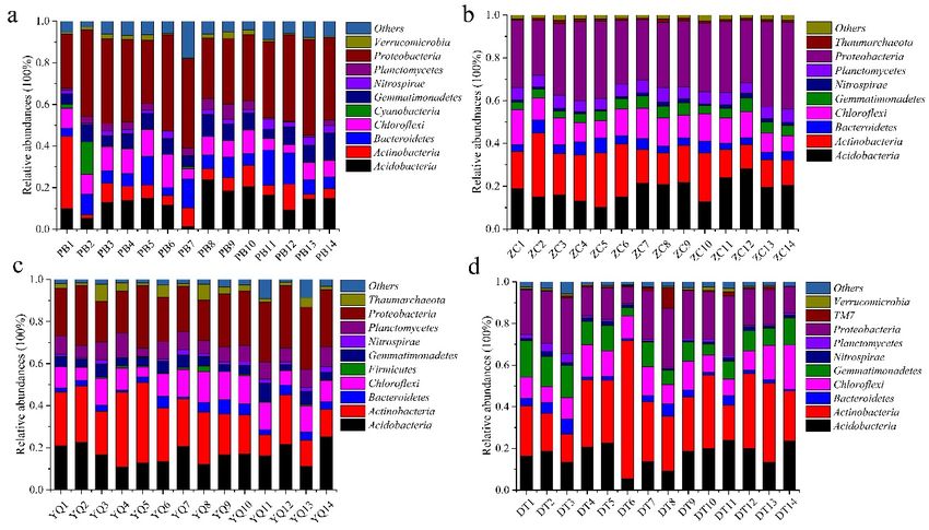
Microorganisms 2020, 8, 433                                                                           5 of 22

indices to reveal the richness, diversity, and evenness of the OTUs and performed beta diversity analysis
online using the open-source platform Metagenomics for Environmental Microbiology (DengLab;
http://mem.rcees.ac.cn:8080/). According to the taxonomic results, we constructed an abundance
diagram and obtained rich infrared images with Origin 9.1 (OriginLab, Northampton, MA, USA)
and R software (https://www.r-project.org/). The principal component analysis (PCA), non-metric
multidimensional scaling (NMDS), response ratio calculation (RRC), canonical correspondence analysis
(CCA), variation partition analysis (VPA), correlation test, mantel test, and LEfSe (linear discriminant
analysis effect size) were also conducted on this platform.

2.3. Network Construction and Analysis
     On the basis of 16S rDNA sequencing data, we used all the data from the 56 collected soil
samples to construct the interaction networks, which we defined as phylogenetic MENs [24]. For these
56 samples, each mining area had 14 samples to establish their own networks.
     According to Deng et al. [25], we followed four steps in the construction process: data collection,
data transformation, pairwise similarity matrix calculation, and adjacent matrix determination. During
the construction, we only used the OTUs (97% sequence identity) occurring in 100% of the total
samples for the network computation. Then, we filled the blanks of 0.01 with paired valid values. As
recommended, we used Spearman’s Rho to measure the correlation and calculated a similarity matrix.
Thereafter, we increased the similarity threshold from 0.01 to 0.99 with intervals of 0.01, and selected an
optimal similarity threshold. We determined significant non-random patterns by evaluating whether
the spacing of the eigenvalue distribution followed a Poisson distribution. In order to allow for a
comparison, we used an identical cutoff of 0.86 to construct the interaction networks for each mining
area. We performed network construction and statistical analysis using the existing pipeline available
at http://ieg4.rccc.ou.edu/mena. We visualized these networks with Cytoscape 3.7.0 software [26].

2.4. Characterization of the Molecular Ecological Networks and Statistical Analysis
     We calculated network global properties, including total nodes and links, R2 of power-law, average
degree (avgK), and average path distance (GD). Then, we calculated network indices for individual
nodes on the pipeline, such as degree and stress centrality. Greedy modularity optimization was
presented as a separation method for module separation. In the network, module was defined as a
group of OTUs with a high connection among themselves, but few connections were made with OTUs
outside the group. Furthermore, modularity (M) was extremely important for system stability [27].
Then we calculated two important parameters, Zi (within-module connectivity) and Pi (among-module
connectivity), for the modularity of all the nodes. According to the values of Zi and Pi, we classified
the roles of nodes into four categories: peripherals (Zi ≤ 2.5, Pi ≤ 0.62), connectors (Zi ≤ 2.5, Pi > 0.62),
module hubs (Zi > 2.5, Pi ≤ 0.62), and network hubs (Zi > 2.5, Pi > 0.62) [22]. Additionally, we fitted
three power-law models for the first step of the network statistics. Then, to evaluate the constructed
networks, we rewired the network connections and calculated the network properties randomly with
100 permutations between random and empirical networks.
     We also calculated the relationships between gene significances (GS) and environmental traits
and used the Mantel test to check for correlations between GS and network connectivity. The GS was
calculated and defined as the square of the Pearson correlation coefficient (R2) of the OTU abundance
profile with environmental traits. We used these correlations between GS and network indices to reveal
the internal associations between network topology and environmental traits. During the process, we
used the Euclidean distance method. Then we ran the process of module-eigengene analyses on the
pipeline. The eigengene analysis was useful in revealing higher-order organizations and to identify key
populations based on network topology. In the analysis, we summarized every module through a single
value decomposition analysis, which we referred to as the module eigengene. The relative abundance
profile of the OTUs within a module could be shown in eigengene. Moreover, the relationships among
eigengenes have been visualized as a clustering dendrogram through average-linkage hierarchical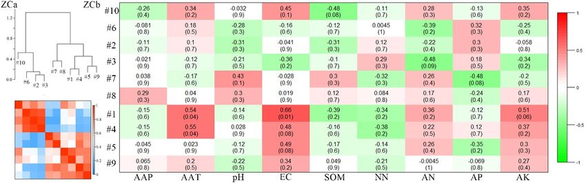
Microorganisms 2020, 8, 433                                                                                           6 of 22

analysis [24]. Additionally, we calculated the relationships between traits and modules, which are
shown in a heatmap.

3. Results

3.1. The Taxonomic Composition of Microbial Consortia in Different Mining Areas
     We analyzed the taxonomy alpha diversity of the soil microbial communities for 56 soil samples
(Table 1). After comparing the Chao and Shannon index for each mining area, we found that soil
bacterial diversity in the Zoucheng (ZC) network was the highest and that in the PB network had the
smallest value. The results implied that the ZC area had the highest species richness and diversity,
whereas Peibei (PB) had the lowest. We used Pielou evenness to measure the heterogeneity of the
community. The data in Table 1 showed that the value of ZC was the highest, which indicated that
the evenness of its microbial community species was the best. Moreover, the values of the Chao and
Shannon index were the smallest in PB, although the value of Pielou evenness was not the smallest.

                Table 1. The alpha diversity index of soil microorganisms in the four mining areas.

      Mining Area             Chao                         Shannon                        Pielou Evenness
      PB                      3710.10 ± 836.20 b           6.5937 ± 0.5738  ab            0.8305 ± 0.0441 c
      ZC                      8319.38 ± 541.91 ab          7.7519 ± 0.0824 c              0.9014 ± 0.0105 bc
      YQ                      4917.14 ± 891.56 c           6.8408 ± 0.2617 bc             0.8463 ± 0.0177 ab
      DT                      5238.99 ± 421.43 bc          6.7701 ± 0.1585 b              0.8120 ± 0.0144 ab
      Mean ± standard deviation (SD) (n = 14). Superscript letters such as a, b and c, indicate significant differences
      between different sampling sites for each parameter separately using Duncan test at significant p < 0.05 level
      (ANOVA analysis, n = 14). PB, ZC, YQ and DT stand for the sampling sites Peibei, Zoucheng, Yangquan and Datong.

      Overall, the bacterial categories were relatively abundant in the 56 soil samples (Figure 2).
Acidobacteria, Actinobacteria, Bacteroidetes, Chloroflexi, Gemmatimonadetes, Nitrospirae, Planctomycetes,
and Proteobacteria accounted for almost 90% of the total sequences in each soil sample. Cyanobacteria,
Candidatus Saccharibacteria (TM7), Firmicutes, Thaumarchaeota, and Verrucomicrobia were present in
some soil samples with little occupation. The most abundant phylum in the PB, ZC, and Yangquan
(YQ) mining areas was Proteobacteria, which accounted for 37.42% ± 6.26%, 32.67% ± 4.13%, and
24.80% ± 3.95%, whereas it was Actinobacteria (29.68% ± 12.37%) was the most abundant in the DT
mining area (Figure 2). Acidobacteria was the second most abundant phylum in PB (the proportion was
just 13.38% ± 5.63%). However, Actinobacteria was found to be the second most abundant phylum in
the ZC and YQ networks. Figure 2a,d also showed that the phylum Cyanobacteria and Verrucomicrobia
accounted for more than 1% in the PB mine, whereas TM7 (1.47% ± 2.39%) was the most present in the
Datong (DT) mine. Phylum Thaumarchaeota appeared in the ZC and YQ mining areas with a proportion
of more than 1%. Furthermore, the proportion of Acidobacteria trended in the order of ZC > DT >YQ >
PB, and Chloroflexi had a similar occupation of around 10%. The proportion of Nitrospirae was shown
to be around 1% in the four mining areas. The proportion of Bacteroidetes trended in the order of
PB > ZC > YQ > DT in the four areas. Moreover, the proportion of Gemmatimonadetes trended in the
order of DT > PB > YQ > ZC, and Planctomycetes trended in the order of YQ > ZC > PB > DT in the four
mining areas. These results suggested that the microbial distribution patterns across spatial distance
varied among the four mining areas, which supported half of the third hypothesis.
      Based on the community structure, principal component analysis (PCA), non-metric
multidimensional scaling (NMDS), and response ratio calculation (RRC) were performed for the
bacterial structure comparison of the four mining areas. The results indicated that the differences
among the microbial structures and compositions were representative. The colorful dots shown in
Figure 3 stand for different samples (or communities). If two dots were closer, it meant that there
was a higher similarity between the microbial community structures of the two samples. The results
of PCA and NMDS analysis showed that the soil microbial communities from the four mining areas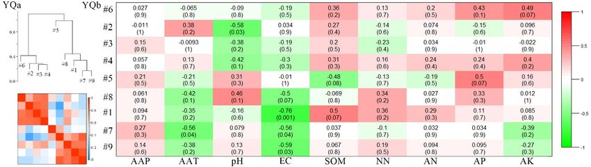
Microorganisms 2020, 8, 433                                                                                     7 of 22

were  different,
Microorganisms    whereas
               2020, 8, x FORthe  bacterial
                               PEER  REVIEWcomposition and structure within each group (mining area)7 were   of 22
 Microorganisms
grouped         2020, It
           closely.   8, xcan
                           FORbePEER
                                  seenREVIEW
                                        that the dot arrangement of PCA represents the distinctive pattern  7 of 22

along
patternthe  vertical
         along         axis, according
                 the vertical             to the location
                                 axis, according            order oforder
                                                   to the location   PB, ZC,  YQ,ZC,
                                                                          of PB,  andYQ,DT.and
                                                                                            However,  the NMDS
                                                                                               DT. However,    the
 pattern showed
analysis  along thethat vertical  axis, according
                            the groups   followed   todifferent
                                                       the location  order of PB,
                                                                               theZC,  YQ, andaxis
                                                                                                DT.separating
                                                                                                    However,the the
NMDS analysis        showed      that the   groupsa followed    pattern, with
                                                                 a different       horizontal
                                                                              pattern,  with the horizontal   axis
 NMDS
four       analysis
     groupsthe along   showed     that  the  groups    followed   a different  pattern,  with the  horizontal  axis
separating        fourthe    spatial
                         groups      order
                                  along     ofspatial
                                          the  PB, ZC,order
                                                        YQ, of
                                                             and  DT.
                                                                PB, ZC, YQ, and DT.
 separating the four groups along the spatial order of PB, ZC, YQ, and DT.

      Figure 2. Bacterial categories ((a), (b), (c), and (d)) in soil samples across Peibei (PB), Zoucheng (ZC),
       Figure2.2.Bacterial
      Figure      Bacterialcategories
                            categories(a–d)
                                       ((a), in
                                             (b),soil
                                                  (c),samples
                                                       and (d))across
                                                                in soilPeibei (PB),
                                                                        samples     Zoucheng
                                                                                 across Peibei(ZC),
                                                                                               (PB),Yangquan
                                                                                                    Zoucheng(YQ),
                                                                                                             (ZC),
                                  Yangquan (YQ), and Datong (DT) mining areas.
      and Datong (DT) mining areas.Yangquan (YQ), and Datong (DT) mining areas.

                              (a)                                                      (b)
                               (a)                                                      (b)
     Figure 3.
     Figure  3. Principal
                Principal component
                          component analysis
                                        analysis (PCA;
                                                  (PCA; (a))
                                                         (a)) and
                                                              and non-metric
                                                                   non-metric multidimensional
                                                                              multidimensional scaling
                                                                                                scaling (NMDS;
                                                                                                        (NMDS;
      Figure 3. Principal component analysis (PCA; (a)) and non-metric multidimensional scaling (NMDS;
                     (b)) analysis  results of soil bacteria at the phylum level
     (b)) analysis results of soil bacteria at the phylum level in mining areas. in mining areas.
                      (b)) analysis results of soil bacteria at the phylum level in mining areas.
3.2. Topological Properties
3.2. Topological Properties of
                            of MENs
                               MENs in
                                    in Different
                                       Different Mining
                                                  Mining Areas
                                                         Areas
 3.2. Topological Properties of MENs in Different Mining Areas
      In
      In recent
         recent years,
                 years, the
                        the method
                             method of
                                    of network    analysis has
                                        network analysis    has been
                                                                been proposed
                                                                     proposed as
                                                                               as aa new
                                                                                     new way
                                                                                          way to
                                                                                               to explore
                                                                                                  explore
       In recent
interaction       years,
             patterns of the  method
                          complicatedof  network
                                       data sets,  analysis
                                                  which  may has been
                                                              provide proposed
                                                                      more      as  a
                                                                           informationnew  way
                                                                                         than   to explore
                                                                                              alpha–beta
interaction patterns of complicated data sets, which may provide more information than alpha–beta
 interaction patterns of complicated data sets, which may provide more information than alpha–beta
diversity analysis. Therefore, in this study, to derive a better understanding of big differences
 diversity analysis. Therefore, in this study, to derive a better understanding of big differences
between the composition and abundance of soil bacterial communities in mining areas, we used
 between the composition and abundance of soil bacterial communities in mining areas, we used
network analyses to explore the associations between soil bacterial taxa in the mining sites.
 network analyses to explore the associations between soil bacterial taxa in the mining sites.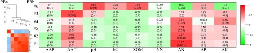
Microorganisms 2020, 8, 433 8 of 22
diversity analysis. Therefore, in this study, to derive a better understanding of big differences between
the composition and abundance of soil bacterial communities in mining areas, we used network
analyses to explore the associations between soil bacterial taxa in the mining sites.
In MENs, the microbial species (meaning nodes) are linked by pairwise interactions (meaning
links), which may reveal some of the biological interactions in the ecosystem. In this study, we
individually constructed four networks from different mining areas. We investigated some important
general network topological features, such as the scale free, small world, or modular, to understand
the differences among these MENs. Table 2 showed that their connectivity followed the power law,
and that the network connectivity (or degree) in the four constructed MENs was fitted well with the
power-law model (R2 values of 0.837–0.931, respectively). The results revealed that all the curves of the
network connectivity distribution were fitted well with the power-law model, which was indicative of
the scale-free networks. Furthermore, the average clustering coefficients and path distances were also
different from those of the corresponding random networks (Table 2).
Table 2. Topological properties of the empirical molecular ecological networks of microbial communities
and their random networks in different mining areas.
Network Indexes PB ZC YQ DT
Similarity threshold 0.86 0.86 0.86 0.86
R2 of power law 0.837 0.931 0.852 0.896
Total nodes 248 265 165 441
Total links 1285 516 163 640
Empirical
Average degree (avgK) 10.363 3.894 1.976 2.902
networks
Average clustering coefficient (avgCC) 0.314 0.258 0.158 0.184
Average path distance (GD) 3.334 7.725 3.975 7.802
Modularity 0.364 0.701 0.897 0.829
Module number (with >5 nodes) 6 10 9 13
Average clustering coefficient (avgCC) 0.134 ± 0.010 0.028 ± 0.006 0.007 ± 0.005 0.008 ± 0.003
Random
Average path distance (GD) 2.772 ± 0.024 3.877 ± 0.058 6.454 ± 0.448 5.022 ± 0.076
networks
Modularity 0.228 ± 0.005 0.496 ± 0.008 0.795 ± 0.011 0.637 ± 0.008
Table 2 showed that the average clustering coefficients (avgCC) of the PB, ZC, YQ, and DT
networks were 0.314, 0.258, 0.158, and 0.184, respectively. The average degrees (avgK) of the PB, ZC,
YQ, and DT networks were 10.363, 3.894, 1.976, and 2.902. The average path distances (GD) of the
PB, ZC, YQ, and DT networks were 3.334, 7.725, 3.975, and 7.802, which were close to the logarithms
of the total number of network nodes, suggesting that the four MENs had the typical property of a
small world. Deng et al. have reported that a higher avgK is indicative of a more complex network
and that a small GD means that nodes in the network are closer [25]. This information shows that
the PB network was the most complex network, and it could be identified by the highest avgK and
shortest GD (Table 2). For modularity, all modularity values ranged from 0.364 to 0.897, which was
higher than the modularity values from their corresponding randomized networks. Therefore, all of
the constructed MENs appeared to be modular. In the PB, ZC, YQ, and DT networks, we focused on
the modules with more than five nodes. As a result, we detected modules 6, 10, 9, and 13 with more
than five nodes. The module sizes varied considerably, ranging from 6 to 73 nodes, and the individual
modules showed obvious differences. Most importantly, all of the results confirmed that the network
properties differed significantly among different mining habitats, which supported the first hypothesis.
3.3. Dominant Microbial Taxa across Different Mining Areas
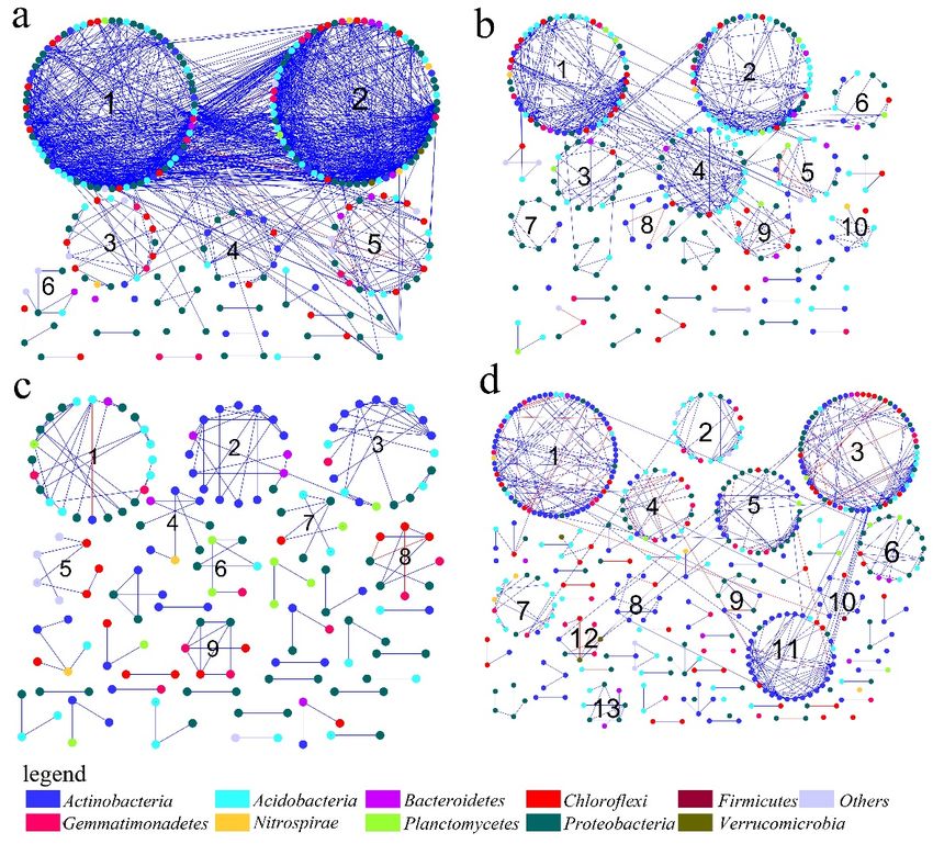
Microbial network structures were distinctly different among the four networks across the different
mining areas, and across the semihumid to semiarid locations in China (Figure 4). Figure 4 showed
that there were eight phyla in each network with node degrees > 1, namely, Acidobacteria, Actinobacteria,
Bacteroidetes, Chloroflexi, Gemmatimonadetes, Nitrospirae Planctomycetes, and Proteobacteria. As reported,
we considered the nodes with higher degrees to be the central nodes in the network structure [28].
Figure 4 also showed that nodes with high connectivity (degree) varied across the mining areas. In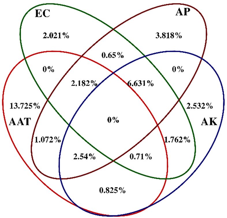
Microbial network structures were distinctly different among the four networks across the
different mining areas, and across the semihumid to semiarid locations in China (Figure 4). Figure 4
showed that there were eight phyla in each network with node degrees > 1, namely, Acidobacteria,
Actinobacteria, Bacteroidetes, Chloroflexi, Gemmatimonadetes, Nitrospirae Planctomycetes, and
Microorganisms 2020, 8, 433 9 of 22
Proteobacteria. As reported, we considered the nodes with higher degrees to be the central nodes in
the network structure [28]. Figure 4 also showed that nodes with high connectivity (degree) varied
across
the the mining
PB network, theareas. In the
top five PB (60>
nodes network,
nodethe top five
degree >40),nodes
which (60> node
might degree
have been>40), which might
the predominant
have been the predominant phylum, belonged to Acidobacteria
phylum, belonged to Acidobacteria (OTU_24020, OTU_19752 and OTU_20695) and Gemmatimonadetes(OTU_24020, OTU_19752 and
OTU_20695)and
(OTU_30606 andOTU_23181;
GemmatimonadetesFile S1 (OTU_30606
in Additionaland file OTU_23181;
1). In the ZC File S1 in Acidobacteria
network, Additional file 1). In the
(OTU_8126,
ZC network, Acidobacteria (OTU_8126, OTU_34138), Chloroflexi (OTU_40961
OTU_34138), Chloroflexi (OTU_40961 and OTU_75010), and Proteobacteria (OTU_59288 and OTU_10968) and OTU_75010), and
Proteobacteria
had a high node (OTU_59288
degree (20>and nodeOTU_10968)
degree >15)had anda played
high node degree (20>
an important node
role (Filedegree >15) and played
S2 in Additional file 2).
In the YQ network, all of the nodes had a smaller node degree, whereas OTU_29287, OTU_61084,node
an important role (File S2 in Additional file 2). In the YQ network, all of the nodes had a smaller and
degree, whereas
OTU_3172 had theOTU_29287, OTU_61084,
top node degrees, and OTU_3172
with values of 7, 6, and had the top node
7, respectively (Filedegrees, with values
S3 in Additional of
file 3).
7, 6, and all
Moreover, 7, respectively (File S3 in
three nodes belonged Additional fileIn3).
to Actinobacteria. theMoreover,
DT network, allOTU_26953
three nodes(Acidobacteria),
belonged to
Actinobacteria. In the DT network, OTU_26953 (Acidobacteria),
OTU_47804 and OTU_21400 (Actinobacteria), and OTU_3503 and OTU_33441 (Chloroflexi) OTU_47804 and OTU_21400
had high
node degrees, with values of 13, 13, 14, 11, and 11 (File S4 in Additional file 4). Compared to values
(Actinobacteria), and OTU_3503 and OTU_33441 (Chloroflexi) had high node degrees, with the node of
13, 13,
sizes of14,
the11, andnetworks,
other 11 (File S4the indegree
Additional
values file
of4).
theCompared
YQ network to were
the node sizes(Figure
smaller of the 4).
other networks,
Furthermore,
the dominant bacterial species for all four networks showed significant changes. These resultsbacterial
the degree values of the YQ network were smaller (Figure 4). Furthermore, the dominant implied
species
that for all mining
different four networks showed
areas were significant
selected changes.
for different These results
bacterial impliedwhich
communities, that different
suggested mining
that
areas were selected for different bacterial communities, which suggested that
the interactions among different microbial taxa in the soil bacterial communities were substantially the interactions among
different according
changed microbial taxa in thethey
to where soil were
bacterial communities
located. were
This result substantially
confirmed changed
the fact according
that the microbial to
where they were
distribution located.
patterns This
across resultdistance
spatial confirmed andthethefact that the microbial
interactions distribution
of the bacterial patternsvaried
communities across
spatial distance and the interactions of the bacterial
among the mining areas, which supported the third hypothesis. communities varied among the mining areas,
which supported the third hypothesis.
Figure 4. Overview of the networks in different mining areas, with node sizes being proportional to
Figure 4. Overview of the networks in different mining areas, with node sizes being proportional to
node degrees. A red link means a negative correlation and a blue link means a positive correlation.
node degrees. A red link means a negative correlation and a blue link means a positive correlation.
The connectivity
The connectivity within
within and
and among
amongmodules
moduleshashasbeen
beenreported
reportedininorder toto
order identify thethe
identify roles of
roles
nodes in the MENs [29]. We used peripherals, connectors, module hubs, or network hubs
of nodes in the MENs [29]. We used peripherals, connectors, module hubs, or network hubs to to assign
every node
assign everyinnode
the ecological networks.
in the ecological In the four
networks. networks,
In the peripherals
four networks, occupiedoccupied
peripherals >96% of >96%
the total
of
the total nodes. Compared to one module hub (OTU_29287) in the YQ network, more module hubs
appeared in the PB (OTU_2777 and OTU_13398), ZC (OTU_10968, OTU_8126, and OTU_59288), and
DT (OTU_26953, OTU_21400, and OTU_40485) networks (File S1–S4 in Additional file 1–4). We
observed some connectors in the PB, ZC, and DT networks, while the YQ network did not have any
connectors (Figure 5). Compared to the module hubs, we detected more connectors, especially in the PB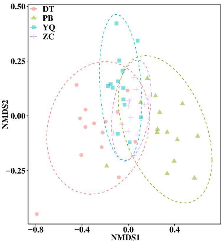
Microorganisms 2020, 8, x FOR PEER REVIEW                                                                                            10 of 22

nodes. Compared to one module hub (OTU_29287) in the YQ network, more module hubs appeared
in the PB (OTU_2777 and OTU_13398), ZC (OTU_10968, OTU_8126, and OTU_59288), and DT
(OTU_26953,2020,
Microorganisms  OTU_21400,
                   8, 433    and OTU_40485) networks (File S1-S4 in Additional file 1–4). We observed 10 of 22
some connectors in the PB, ZC, and DT networks, while the YQ network did not have any connectors
(Figure 5). Compared to the module hubs, we detected more connectors, especially in the PB network,
network, which had nine connectors. Figure 5 also showed that the module hubs and connectors had a
which had nine connectors. Figure 5 also showed that the module hubs and connectors had a wide
wide distribution in various microbial populations. Of the total nine module hubs, three belonged to
distribution in various microbial populations. Of the total nine module hubs, three belonged to
Acidobacteria, three to Actinobacteria, one to Chloroflexi, and two to Proteobacteria. Nine connectors in the
Acidobacteria, three to Actinobacteria, one to Chloroflexi, and two to Proteobacteria. Nine connectors in
PB network belonged to the bacterial phyla Acidobacteria, Actinobacteria, Bacteroidetes, Chloroflexi, and
the PB network belonged to the bacterial phyla Acidobacteria, Actinobacteria, Bacteroidetes, Chloroflexi,
Proteobacteria. Moreover, two connectors, which were Actinobacteria and Chloroflexi, were shown in
and Proteobacteria. Moreover, two connectors, which were Actinobacteria and Chloroflexi, were shown
the ZC network, whereas the two connectors identified in the DT network both belonged to phylum
in the ZC network, whereas the two connectors identified in the DT network both belonged to
Acidobacteria. A notable phenomenon was that we did not identify a network hub in the four networks.
phylum Acidobacteria. A notable phenomenon was that we did not identify a network hub in the four
The result suggested that Acidobacteria occupied the first percentage of the module hubs and connectors,
networks. The result suggested that Acidobacteria occupied the first percentage of the module hubs
then followed then by Actinobacteria, Chloroflexi, and Proteobacteria. Furthermore, phyla Bacteroidetes
and connectors, then followed then by Actinobacteria, Chloroflexi, and Proteobacteria. Furthermore,
appeared just once.
phyla Bacteroidetes appeared just once.

                                                 5
                                                      Module hubs Acido, Chloro                           Network hubs
                                                                   Acido, Proteo*2
                                                                                                                              PB
                                                 4                 Actino                                                     ZC
               Within-module connectivity (Zi)

                                                                   Acido, Actino*2                                            YQ
                                                 3                                                                            DT

                                                                                                          Connectors
                                                 2                                                             Acido*2, Actino*2,
                                                                                                               Bacteroi, Chloro*2,
                                                 1                                                             Proteo*2
                                                                                                               Actino, Chloro
                                                                                                               Acido*2
                                                 0

                                                 -1

                                                 -2 Peripherals

                                                  -0.1     0.0     0.1  0.2   0.3    0.4    0.5     0.6      0.7       0.8
                                                                      Among-module connectivity (Pi)

     Figure 5. Z–P plot showing the keystone species in the different mining area networks. Different
     Figure 5. Z–P plot showing the keystone species in the different mining area networks. Different
     symbols with special colors represent different networks as follows: black star for the PB network, red
     symbols with special colors represent different networks as follows: black star for the PB network,
     circle for the ZC network, blue upward-facing triangles for the YQ network, and rose downward-facing
     red circle for
     triangles   for the
                     the ZC
                          DTnetwork,
                              network.blue upward-facing
                                         The  module hubstriangles for the YQare
                                                            and connectors    network,
                                                                                 labeledand  rose
                                                                                          with    downward-
                                                                                                phylogenetic
     facing triangles
     affiliations       for the DT network.
                  (Acido—Acidobacteria,      The module hubs Bacteroi—Bacteroidetes,
                                        Actino—Actinobacteria, and connectors are labeled  with phylogenetic
                                                                                     Chloro—Chloroflexi, and
     affiliations  (Acido—Acidobacteria,   Actino—Actinobacteria, Bacteroi—Bacteroidetes, Chloro—Chloroflexi,
     Proteo—Proteobacteria. *2 means that there are 2 connectors or 2 module hubs belong to that phylum).
     and Proteo—Proteobacteria. *2 means that there are 2 connectors or 2 module hubs belong to that
     phylum).
     As shown in Figure 6a, in the PB network, the nodes with a high degree belonged to modules 1
and 2, including Acidobacteria (OTU_24020, OTU_19752, OTU_20695, OTU_13398, and OTU_23653)
      As shown in Figure
and Gemmatimonadetes         6a, in the PB
                          (OTU_30606     andnetwork,   the nodes
                                              OTU_23181).          with OTU_13398
                                                              Notably,   a high degree   belonged
                                                                                      also  workedto  asmodules
                                                                                                         a module1
 and  2, including   Acidobacteria (OTU_24020,     OTU_19752,      OTU_20695,    OTU_13398,
hub. Moreover, OTU_19164, which was identified as the phylum Nitrospirae from module 2, had a   and   OTU_23653)
 and Gemmatimonadetes
high   degree, in addition(OTU_30606
                             to OTU_27917and OTU_23181).      Notably,
                                               (Proteobacteria)          OTU_13398
                                                                 and OTU_22409         also worked asIn
                                                                                    (Actinobacteria).     a module
                                                                                                             the ZC
network, the nodes with a high degree were primarily distributed in modules 1 and 2, which had
 hub.  Moreover,    OTU_19164,    which    was  identified as the   phylum   Nitrospirae  from  module      2,  werea
 high  degree,   in addition  to OTU_27917      (Proteobacteria)  and  OTU_22409     (Actinobacteria).
identified as phyla Chloroflexi (OTU_40961 and OTU_75010), Acidobacteria (OTU_8126 and OTU_34138),       In  the  ZC
 network,
and         the nodes
      Proteobacteria    with a highand
                     (OTU_10968       degree  were primarily
                                         OTU_59288).             distributed
                                                          OTU_8126     had theinhighest
                                                                                 modules    1 andand
                                                                                         degree     2, which
                                                                                                        worked  were
                                                                                                                   as
 identified   as   phyla  Chloroflexi   (OTU_40961      and   OTU_75010),       Acidobacteria
the module hub, although OTU_10968 and OTU_59288 also served as module hubs (Figure 6b). In     (OTU_8126        and
 OTU_34138),
the YQ network  and(Figure
                     Proteobacteria
                            6c), the(OTU_10968
                                     nodes all had and  OTU_59288).
                                                     a small            OTU_8126tohad
                                                              degree compared         thethe  highest
                                                                                           other  threedegree    and
                                                                                                         networks.
 worked as the
OTU_29287,        module
               shown      hub, althoughhad
                      as Actinobacteria,   OTU_10968     and
                                               the highest   OTU_59288
                                                           degree          also served
                                                                    and worked    as theas  module
                                                                                         module       hubs
                                                                                                    hub.  In (Figure
                                                                                                              the DT
 6b). In  the YQ   network  (Figure   6c), the  nodes  all had  a  small  degree  compared     to
network, the nodes with high degree were primarily distributed in modules 1, 3, and 11, which were the  other   three
 networks.    OTU_29287,   shown    as Actinobacteria,  had  the  highest  degree  and   worked
shown as phyla Actinobacteria (OTU_47804, OTU_21400, and OTU_40485), Acidobacteria (OTU_26953),     as the  module
and Chloroflexi (OTU_3503 and OTU_33441). Notably, OTU_21400 had the highest degree and worked
as the module hub, whereas OTU_26953 and OTU_40485 played the roles of module hubs (Figure 6d).
hub. In the DT network, the nodes with high degree were primarily distributed in modules 1, 3, and
11, which were shown as phyla Actinobacteria (OTU_47804, OTU_21400, and OTU_40485),
Acidobacteria (OTU_26953), and Chloroflexi (OTU_3503 and OTU_33441). Notably, OTU_21400 had the
Microorganisms
highest degree 2020,
and8, 433
worked as the module hub, whereas OTU_26953 and OTU_40485 played the11roles
of 22
of module hubs (Figure 6d).
Figure 6.6.Network
Figure Networkgraph withwith
graph module structure
module produced
structure by the fast-greedy
produced by the modularity
fast-greedy optimization
modularity
method.
optimization method. Each node corresponds to a microbial population. Arable as
Each node corresponds to a microbial population. Arable numbers such 1, 2, 3, and
numbers such4 stands
as 1, 2,
for the module number. A red link indicates a negative correlation, and a blue link indicates
3, and 4 stands for the module number. A red link indicates a negative correlation, and a blue link a positive
correlation.
indicates a (a–d) stand
positive for the PB,(a),
correlation. ZC,(b),
YQ,(c),
and DT(d)
and network,
stand respectively.
for the PB, ZC, YQ, and DT network,
respectively.
3.4. Eigengene Network Analysis
Module 6 Network
3.4. Eigengene in FigureAnalysis
S1 illustrated a conceptual example of eigengene network analysis (Figure S1–S4
in Additional file 5–8). The eigengene network analysis was composed of various components. In
Module 6 in Figure S1 illustrated a conceptual example of eigengene network analysis (Figure
module 6, for example, the heatmap showed the standardized relative abundances (SRAs) of bacterial
S1–S4 in Additional file 5–8). The eigengene network analysis was composed of various components.
species across 14 samples within module 6 in the PB network. In the heatmap, each row corresponded
In module 6, for example, the heatmap showed the standardized relative abundances (SRAs) of
to the individual OTUs in module 6, whereas columns indicated the 14 samples in the PB network. The
bacterial species across 14 samples within module 6 in the PB network. In the heatmap, each row
SRA of the corresponding eigengene (y-axis) across the samples (x-axis) were also shown in module 6.
corresponded to the individual OTUs in module 6, whereas columns indicated the 14 samples in the
Figure S1 showed that only five microbes had significant module memberships, where the y-axis
PB network. The SRA of the corresponding eigengene (y-axis) across the samples (x-axis) were also
shows the SRAs and the x-axis shows the individual samples. The values in parentheses are module
shown in module 6. Figure S1 showed that only five microbes had significant module memberships,
memberships, and the module memberships included in the analysis correspond to the key species
where the y-axis shows the SRAs and the x-axis shows the individual samples. The values in
within a module. We examined module membership, which is shown as the square of the Pearson
parentheses are module memberships, and the module memberships included in the analysis
correlation between the given species abundance profile and the module eigengene. We identified
correspond to the key species within a module. We examined module membership, which is shown
significant module memberships within the respective modules (File S5–S8 in Additional file 9–12).
as the square of the Pearson correlation between the given species abundance profile and the module
In this study, there were 6, 10, 9, and 13 modules in the eigengene analysis of the PB, ZC, YQ, and
eigengene. We identified significant module memberships within the respective modules (File S5–S8
DT networks, respectively. The module eigengenes explained 53%–81%, 61%–77%, 53%–81%, and
in Additional file 9–12).
52%–70% of the variations in relative species abundance across the different samples in the PB, ZC, YQ,
and DT networks, respectively (Figure S1–S4 in Additional file 5–8). All of the eigengenes explicated
over 50% of the observed variations, which revealed that these eigengenes could represent species
shift across different samples in the individual modules.Microorganisms 2020, 8, 433 12 of 22
Microorganisms 2020, 8, x FOR PEER REVIEW 12 of 22
InThe
thismeta-modules
study, there were 6, 10, 9,
were shown asand
groups13 modules in the
of eigengenes eigengene analysis
in dendrogram of the PB,
in the eigengene ZC, YQ,
network,
which implied the higher-order structure of the constructed network.
and DT networks, respectively. The module eigengenes explained 53%–81%, 61%–77%, 53%–81%, In this study, the eigengenes
andfrom the modules
52%–70% of theshowed
variationssignificant correlations.
in relative Many meta-modules
species abundance were clustered
across the different samplesfor in
thethe
ZC,PB,
YQ, and DT networks, whereas only one meta-module was clustered for
ZC, YQ, and DT networks, respectively (Figure S1–S4 in Additional file 5–8). All of the eigengenesthe PB network (Figure 7a).
The eigengenes from the paired modules were clustered differently in the
explicated over 50% of the observed variations, which revealed that these eigengenes could representdifferent networks, which
implied
species that
shift the higher
across differentorder organization
samples of the paired
in the individual modules was totally different among the
modules.
different mining areas. Otherwise, to check
The meta-modules were shown as groups of eigengenes which property was in most important for
dendrogram the network
in the eigengene
modules, we investigated the trait-based module significances, by squaring the correlation between
network, which implied the higher-order structure of the constructed network. In this study, the
signal intensity of the modules and some soil characteristics, including the climate parameters of AAP
eigengenes from the modules showed significant correlations. Many meta-modules were clustered
(annual average precipitation) and AAT (annual average temperature; Figure 7b). Figure 7b showed
for the ZC, YQ, and DT networks, whereas only one meta-module was clustered for the PB network
that strongly significant or significant correlations existed for the PB network between the connectivity
(Figure 7a). The eigengenes from the paired modules were clustered differently in the different
of the five modules and the selected variables, including AAT, pH, SOM (soil organic matter), and
networks, which implied that the higher order organization of the paired modules was totally
AN (ammonium nitrate; p ≤ 0.001, 0.001 ≤ p ≤ 0.05). For the ZC network, the connectivity of only one
different among the different mining areas. Otherwise, to check which property was most important
module was significantly related to the AAT and EC (electrical conductivity) values (0.001 ≤ p ≤ 0.05).
forNothe network modules, we
significant correlations wereinvestigated the trait-based
observed, however, between the module significances,
connectivity of all thebymodules
squaringandthe
correlation between
the properties in thesignal intensity
YQ network (p >of0.05).
the For
modules
the DTand some the
network, soilconnectivity
characteristics, including
of three modulesthe
climate parameters of AAP (annual average precipitation) and AAT (annual
showed significant correlation with the selected variables, such as pH, AP (available phosphorus), and average temperature;
Figure 7b). Figure
AK (available 7b showed
potassium; that
0.001 ≤ pstrongly
≤ 0.05). significant or significant
Moreover, these correlations
results indicated existed
that these for the PB
properties,
network
which correlated with the keystone bacterial community were totally different in different AAT,
between the connectivity of the five modules and the selected variables, including mining pH,
SOM (soil
areas, organic
thus matter),
supporting theand AN hypothesis.
second (ammonium nitrate; p ≤0.001, 0.001 ≤ p ≤ 0.05). For the ZC network,
the connectivity
On the other side, a Mantel test andwas
of only one module significantly
correlation test wererelated to the
performed AAT and
to screen for theECdominant
(electrical
conductivity)
environmental values (0.001
factors, which≤ paffected
≤ 0.05).the
Nosoilsignificant
microbialcorrelations were observed,
community structure. however,
The results between
were shown
theinconnectivity
Tables S1 andof S2.allThe
theMantel
modules test showed
and the that microorganisms
properties in the YQ were closely (p
network correlated
> 0.05). with
For AAP,
the DT
AAT, EC,
network, NN,
the AP, and AKof(pthree
connectivity < 0.05; Table S1showed
modules in Additional file 13).correlation
significant Accordingwithto thethe
Pearson
selectedcorrelation
variables,
coefficient and significance, a correlation test presented the results that,
such as pH, AP (available phosphorus), and AK (available potassium; 0.001 ≤ p ≤ 0.05). Moreover, AAP, AAT, EC, AN, AP, and
AK had significant impacts on the structural differentiation of bacterial compositions
these results indicated that these properties, which correlated with the keystone bacterial community (Table S2 in
Additional
were file 14). in different mining areas, thus supporting the second hypothesis.
totally different
Figure 7. Cont.Microorganisms 2020, 8, 433 13 of 22
Microorganisms 2020, 8, x FOR PEER REVIEW 13 of 22
Figure
Figure7.7.Correlations
Correlationsand
and heatmap
heatmap of module
module eigengenes
eigengenesofofthethefour
four networks
networks (a).(a). Correlations
Correlations
between
betweenthethesignal
signalintensity
intensity of
of aa module and each
module and eachsoil
soilcharacteristic
characteristicforfor the
the four
four networks
networks (b).(b).
According
On the othertoside,
abovea results,
MantelCCA and VPA
test and were performed
correlation test weretoperformed
analyze theto
correspondence
screen for thebetween
dominant
the environmental factors and microbial community groups for the four mining areas
environmental factors, which affected the soil microbial community structure. The results (Figure 8). As
were
shown in Figure 8a, samples from the ZC and YQ groups were almost gathered, while
shown in Tables S1–S2. The Mantel test showed that microorganisms were closely correlated PB and DT were
with
separated with them. The correlation information between environmental factors and communities
AAP, AAT, EC, NN, AP, and AK (p < 0.05; Table S1 in Additional file 13). According to the Pearson
can be expressed by the angle between the environmental factor arrow line and the linking line, which
correlation coefficient and significance, a correlation test presented the results that, AAP, AAT, EC,
connected the sample points and center points. Therefore, on the left part of Figure 8a, the correlations
AN, AP, and AK had significant impacts on the structural differentiation of bacterial compositions
between AAT and PB communities were the largest compared to the EC value and AK, while AP had a
(Table S2 in Additional file 14).
closer relationship with YQ and ZC groups. Based on the results of CCA, AAT presented the highest
According to above results, CCA and VPA were performed to analyze the correspondence
explanation percentage for the analysis between environmental factors and microbial communities,
between
followedtheby environmental factors8b).
AP > AK > EC (Figure and microbial community groups for the four mining areas
(Figure 8). As shown in Figure 8a, samples from the ZC and YQ groups were almost gathered, while
PB and DT were separated with them. The correlation information between environmental factors
and communities can be expressed by the angle between the environmental factor arrow line and the
linking line, which connected the sample points and center points. Therefore, on the left part of Figure
8a, the correlations between AAT and PB communities were the largest compared to the EC value
and AK, while AP had a closer relationship with YQ and ZC groups. Based on the results of CCA,
AAT presented the highest explanation percentage for the analysis between environmental factors
and microbial communities, followed by AP > AK > EC (Figure 8b).You can also read