The Antarctic Ice Sheet response to glacial millennial-scale variability
←
→
Page content transcription
If your browser does not render page correctly, please read the page content below
Clim. Past, 15, 121–133, 2019
https://doi.org/10.5194/cp-15-121-2019
© Author(s) 2019. This work is distributed under
the Creative Commons Attribution 4.0 License.

The Antarctic Ice Sheet response to glacial millennial-scale
variability
Javier Blasco1,2 , Ilaria Tabone1,2 , Jorge Alvarez-Solas1,2 , Alexander Robinson1,2 , and Marisa Montoya1,2
1 Departamento   de Fisica de la Tierra y Astrofisica, Facultad de Ciencias Fisicas, Universidad Complutense de Madrid,
28040 Madrid, Spain
2 Instituto de Geociencias, Consejo Superior de Investigaciones Cientificas-Universidad Complutense de Madrid,

28040 Madrid, Spain

Correspondence: Javier Blasco (jablasco@ucm.es)

Received: 1 August 2018 – Discussion started: 23 August 2018
Revised: 28 November 2018 – Accepted: 13 December 2018 – Published: 17 January 2019

Abstract. The Antarctic Ice Sheet (AIS) is the largest ice          1   Introduction
sheet on Earth and hence a major potential contributor to fu-
ture global sea-level rise. A wealth of studies suggest that        The Antarctic Ice Sheet (AIS) presently stores around 60 m
increasing oceanic temperatures could cause a collapse of its       of potential sea-level rise (Fretwell et al., 2013). It is di-
marine-based western sector, the West Antarctic Ice Sheet,          vided into two parts, the East Antarctic Ice Sheet (EAIS) and
through the mechanism of marine ice-sheet instability, lead-        the West Antarctic Ice Sheet (WAIS), including the Antarc-
ing to a sea-level increase of 3–5 m. Thus, it is crucial to        tic Peninsula (AP). Present-day observations show that the
constrain the sensitivity of the AIS to rapid climate changes.      mass balance of the AIS is negative due to mass loss from
The last glacial period is an ideal benchmark period for this       the WAIS, whereas the EAIS maintains a positive mass bal-
purpose as it was punctuated by abrupt Dansgaard–Oeschger           ance (Martín-Español et al., 2016; Shepherd et al., 2018).
events at millennial timescales. Because their center of ac-        Because ablation in the AIS is almost negligible except in
tion was in the North Atlantic, where their climate impacts         the small region of the AP, the mechanisms that contribute to
were largest, modeling studies have mainly focused on the           mass loss are submarine melting of floating ice shelves and
millennial-scale evolution of Northern Hemisphere (NH) pa-          calving processes at the ice front (Paolo et al., 2015; Rignot
leo ice sheets. Sea-level reconstructions attribute the origin      et al., 2013). The WAIS is a marine ice sheet, i.e., most of
of millennial-scale sea-level variations mainly to NH pa-           it is grounded below sea level, and it contains several large
leo ice sheets, with a minor but not negligible role of the         ice shelves that are thinning or calving more rapidly than
AIS. Here we investigate the AIS response to millennial-            the storage provided by surface accumulation. The positive
scale climate variability for the first time. To this end we use    mass balance of the EAIS can be explained by the fact that
a three-dimensional, thermomechanical hybrid, ice sheet–            the amount of floating ice is considerably smaller than in the
shelf model. Different oceanic sensitivities are tested and         WAIS, and thus the mass loss via calving and basal melting
the sea-level equivalent (SLE) contributions computed. We           does not surpass the accumulation.
find that whereas atmospheric variability has no appreciable           Rising oceanic temperatures in the coming century in re-
effect on the AIS, changes in submarine melting rates can           sponse to climate change can boost basal melt and reduce
have a strong impact on it. We show that in contrast to the         ice shelves. Although thinning of floating ice shelves does
widespread assumption that the AIS is a slow reactive and           not directly contribute to sea-level rise, it can lead to a re-
static ice sheet that responds at orbital timescales only, it can   duction of ice-shelf buttressing, enhancing inland ice flow as
lead to ice discharges of around 6 m SLE, involving substan-        seen after the collapse of the Larsen B ice shelf (Fürst et al.,
tial grounding line migrations at millennial timescales.            2016; Rignot et al., 2004) and Pine Island Glacier (Favier
                                                                    et al., 2014; Jacobs et al., 2011). In addition, most parts of
                                                                    the WAIS lie on a retrograde bed slope. Conceptual mod-

Published by Copernicus Publications on behalf of the European Geosciences Union.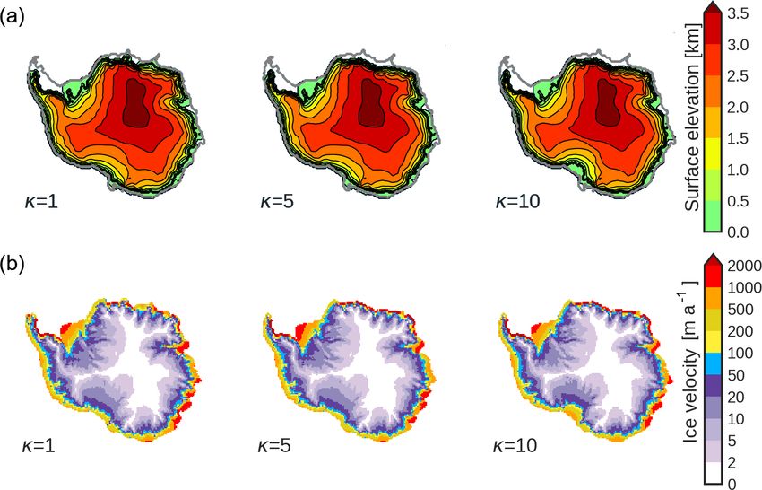
122                                                                         J. Blasco et al.: The Antarctic Ice Sheet response

els suggest the existence of an inherent instability in such       lished (Blunier and Brook, 2001; EPICA Community Mem-
ice sheets, the marine ice-sheet instability (MISI; Weertman,      bers, 2006). The paradigm to explain it is that intensifica-
1974; Schoof, 2007), that could lead to a collapse of the          tions of the AMOC translate into an increase in northward
marine grounded zones in the WAIS region. Mercer (1978)            heat transport at the expense of the southernmost latitudes;
speculated about the fact that this instability could be trig-     conversely, a weakening of the AMOC reduces northward
gered through a rise in oceanic temperatures. Collapse of          heat transport, thereby warming the south (Crowley, 1992;
the WAIS sector could cause a sea-level increase of 3–5 m          Stocker, 1998). The different timescale between northern and
(Bamber et al., 2009; Feldmann and Levermann, 2015; Sut-           southern latitudes can be explained by the fact that the South-
ter et al., 2016), with major implications for coastal zones       ern Ocean (SO) acts as a heat reservoir that dampens and in-
(Nicholls and Cazenave, 2010). From a modeling perspec-            tegrates in time the more rapid North Atlantic signal (Stocker
tive, projections differ considerably in future sea-level con-     and Johnsen, 2003). The occurrence of H events supports a
tributions depending on the model used and the process pa-         high sensitivity of Northern Hemisphere (NH) ice sheets as
rameterizations therein (Bakker et al., 2017a, b; DeConto and      well as their capability to react rapidly (Alvarez-Solas et al.,
Pollard, 2016; Golledge et al., 2015).                             2013, 2017; Andrews and Voelker, 2018; Hemming, 2004).
   Improving our understanding of the AIS sensitivity is           In the Southern Hemisphere (SH), data showing IRD depo-
thus essential to constrain future projections (Bakker et al.,     sition from the AIS are more scarce. There is evidence of
2017a). Some of the most remarkable abrupt climate changes         ice discharges from the AIS (Kim et al., 2018; Weber et al.,
of the near past are those of the last glacial period (LGP;        2012, 2014), but neither a quantification of their contribu-
110–10 ka). Thus, one way to gain insight in this respect is       tion in terms of its sea-level equivalent (SLE) nor the iden-
to assess the response of the AIS to these past rapid climate      tification of their triggering mechanism has yet been done,
changes. In addition, understanding the AIS behavior during        particularly for events during Marine Isotope Stage 3 (MIS-
these millennial-scale abrupt events will help in identifying      3). If a periodic deposition of IRD could be found in the SH
the ultimate causes of the Dansgaard–Oeschger (DO) events.         analogous to the NH, it may hint at an Antarctic response to
Ice-core records from the Greenland Ice Sheet (GrIS) dur-          oceanic changes. This would consolidate the mechanism of
ing the LGP show the characteristic signal of DO events: a         the bipolar seesaw and the existence of the heat storage in the
rapid warming of more than 10 K on decadal timescales fol-         SO.
lowed by a slow cooling that can last from several centuries           Finally, sea-level reconstructions show fast variations of
to thousands of years (e.g., Dansgaard et al., 1993). Model-       more than 20 m at millennial timescales during MIS-3
ing studies (e.g., Ganopolski and Rahmstorf, 2001; Rahm-           (Frigola et al., 2012; Grant et al., 2012; Rohling et al., 2014)
storf, 2002; Shaffer et al., 2004) and reconstructions (Barker     and rises of 4 m per century during meltwater pulse (MWP)
et al., 2015; Böhm et al., 2015; Henry et al., 2016; McManus       1A at ca. 14.5 ka (Liu et al., 2016) . However, the individual
et al., 2004) support the hypothesis that DO events were           contribution of each paleo ice sheet remains unclear. Due to
caused by reorganizations of the Atlantic Meridional Over-         their location at lower latitudes compared to the AIS, NH ice
turning Circulation (AMOC), with enhanced (reduced) North          sheets are more exposed to mass losing processes through at-
Atlantic Deep Water (NADW) formation during interstadials          mospheric forcing (ablation). Therefore the majority of those
(stadials) transporting more (less) heat into high northern lat-   rapid changes are thought to originate in the NH ice sheets
itudes. In addition, marine sediment records across large ar-      (Arz et al., 2007; Ganopolski et al., 2010). However, during
eas of the North Atlantic show quasi-periodic deposition of        MIS-3 sea-level variations fluctuated on the Antarctic rhythm
ice-rafted detritus (IRD) (Hemming, 2004) known as Hein-           (Grant et al., 2012; Rohling et al., 2009; Siddall et al., 2008),
rich (H) events. H events are thought to have been caused          suggesting that a considerable contribution from direct AIS
by massive iceberg discharges from the paleo Laurentide Ice        waxing and waning cannot be excluded.
Sheet (LIS), possibly in response to reductions in NADW                As far as we know, there have been no attempts to simulate
formation that, through positive feedbacks, resulted in the        Antarctic sea-level contributions at millennial timescales and
collapse of the AMOC (Alvarez-Solas et al., 2011, 2013;            their potential implications. The aim of this paper is thus to
Marcott et al., 2013).                                             investigate the response of the AIS to millennial-scale vari-
   Compared to ice-core records in the GrIS, AIS ice-core          ability during the LGP. In particular, we focus on the AIS
records show a more gradual and symmetric sawtooth-like            advance and retreat and its potential sea-level contribution at
signal throughout the whole LGP. An increase in surface            these timescales. Some assumptions are made for the sake
air temperature (SAT) is observed during Greenland stadi-          of simplicity, since our aim is to test if the AIS is likely
als, most notably during Heinrich stadials, with cooling dur-      to have responded at millennial timescales and to what ex-
ing interstadials. The amplitude of this signal can reach up       tent. For this purpose we use a three-dimensional, thermo-
to 2 K (Augustin et al., 2004; Petit et al., 1999; Ruth et al.,    mechanical, ice sheet–shelf model that is forced through a
2007) and the peaks of the sawtooth signal are known as            synthetic climatic forcing including both atmospheric and
Antarctic isotope maxima (AIM). This bipolar seesaw be-            oceanic changes that evolve temporally through an index de-
havior between Greenland and Antarctica is now well estab-         duced from the Dome C deuterium ice-core record. To study

Clim. Past, 15, 121–133, 2019                                                                  www.clim-past.net/15/121/2019/
J. Blasco et al.: The Antarctic Ice Sheet response                                                                             123

the impact of ice–ocean interactions we use a basal melting         enough (200 m) and the incoming ice from upstream does not
parameterization that is a function of oceanic temperature          maintain the necessary ice thickness (Peyaud et al., 2007).
anomalies.
   The paper is structured as follows: first, the ice-sheet         2.2   Forcing method and experimental design
model, the forcing, and the experimental design are described
(Sect. 2). Then the response of the AIS to the oceanic forcing      GRISLI-UCM is forced through the same parameterization
is shown, focusing on the ice discharges and grounding line         for atmospheric and oceanic forcing as in Banderas et al.
advances at millennial timescales (Sect. 3). Finally, the main      (2018) and Tabone et al. (2018), who used it to specifically
results are discussed (Sect. 4) and conclusions summarized          investigate the past evolution of the glacial NH and Green-
(Sect. 5).                                                          land ice sheets, respectively, but here for the Antarctic do-
                                                                    main. In the more general approach used in those studies,
                                                                    oceanic, atmospheric, and precipitation fields are scaled by
2     Methods and experimental setup                                two climatic indices, an orbital index α(t) (where α = 0 rep-
                                                                    resents the LGM state and α = 1 the present day, PD), and a
2.1    Model                                                        millennial index β(t) (β = 0 at the LGM, β = 1 at the AIM).
We use the three-dimensional, hybrid, thermomechanical              Because our study focuses on millennial-scale variability, we
ice-sheet model GRISLI-UCM based on the GRISLI model                fix α = 0 to maintain constant glacial background conditions.
developed by Ritz et al. (2001) and further extended and            The β index is extracted from the Dome C atmospheric tem-
tested at the Complutense University of Madrid (see Alvarez-        perature reconstruction (Jouzel and Masson-Delmotte, 2007)
Solas et al., 2017; Tabone et al., 2018). Important changes         and is filtered between 1 and 19 ka to avoid both orbital and
with respect to the original code include variations in bound-      submillennial-scale variability. The time evolution of atmo-
ary conditions (surface mass balance and basal melt), topog-        spheric temperature (T atm (t)) and precipitation (P (t)) fields
raphy, and new auxiliary modules to calculate the basal drag.       is given by the following equations:
Simulations are run on a 40 km × 40 km grid with 21 ver-
                                                                    T atm (t) = TLGM
                                                                                 atm           atm
                                                                                     + β(t)1Tmil   ,                            (1)
tical layers corresponding to 157 × 147 grid points cover-
ing the whole Antarctic domain. Initial topographic condi-          P (t) = PLGM [(1 − β(t)) δPorb + β(t)δPmil ] ,              (2)
tions (ice thickness, surface, and bedrock elevation) are pro-      where temperature and precipitation, TLGM atm and P
                                                                                                                         LGM , re-
vided from the dataset RTopo-2 (Schaffer et al., 2016), which       spectively, are the LGM climatologies calculated from the
relies on Bedmap2 (Fretwell et al., 2013) with corrections          ERA-Interim reanalysis (Dee et al., 2011) and corrected
for ice-shelf cavities. The grounded slow-moving ice, whose         with orbital anomaly fields obtained from the climatic model
flow is dominated by shear processes, is computed by the            of intermediate complexity CLIMBER 3-α (Montoya and
non-sliding shallow ice approximation (SIA), whereas float-         Levermann, 2008). The millennial (1Tmil  atm , δP ) anomaly
                                                                                                                     mil
ing ice shelves, whose evolution is determined by stretch-          fields are obtained from the same climatic model.
ing processes, are solved by the shallow shelf approximation           The parameterization of the submarine melting rate un-
(SSA) (Hutter, 1983; MacAyeal, 1989). Intermediate states,          der floating ice shelves follows a simple linear law based on
in which shearing and stretching regimes can appear simulta-        Beckmann and Goosse (2003):
neously, are typical of fast-flowing ice streams and are eval-
                                                                    B = κ T ocn − Tf ,

uated by summing the velocities of the SIA and SSA. The                                                                        (3)
SSA solution allows for basal sliding and thus includes basal
drag depending on the topographic conditions. The model al-         where T ocn is the oceanic temperature at the correspond-
lows basal sliding when the ice base (land–ice interface) is at     ing grid point, Tf the freezing point temperature at which
the melting point and the pressure of the basal water exceeds       the ice base is assumed to be, and κ the heat flux exchange
an imposed threshold.                                               coefficient between ocean and ice. Other possible choices
   The total mass balance is given by the difference between        are, for example, a quadratic approach (DeConto and Pol-
accumulation and ablation at the surface, melting at the base       lard, 2016; Pattyn, 2017; Pollard and DeConto, 2009). For
of the ice sheet, and ice discharge into the ocean via calv-        the sake of simplicity, we assume a linear response between
ing. The surface mass balance (SMB) is determined by at-            oceanic temperatures and melting rates, which was already
mospheric temperature and precipitation using the positive          tested previously (Alvarez-Solas et al., 2013; Golledge et al.,
degree-day scheme (Reeh, 1989). The geothermal heat flux            2015; Philippon et al., 2006; Tabone et al., 2018). The model
applied as a boundary condition to grounded ice is obtained         distinguishes between basal melting at the grounding line
from the field provided by Shapiro and Ritzwoller (2004).           (Bgl ) and below the ice shelf (Bshlf ).
Submarine melt is determined through a linear equation,             Bshlf = γ Bgl                                               (4)
which transforms oceanic temperature anomalies into melt-
ing rates through a heat flux coefficient (details in Sect. 2.2).   Rignot and Jacobs (2002) have shown that melting rates at
Calving occurs when the ice-shelf front grid point gets thin        the ice shelves are about an order of magnitude lower than

www.clim-past.net/15/121/2019/                                                                    Clim. Past, 15, 121–133, 2019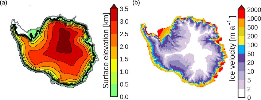
124                                                                         J. Blasco et al.: The Antarctic Ice Sheet response

those close to the grounding line, and hence we set γ to 0.1.
Following the same procedure as for the atmospheric forcing,
the oceanic temperature can be rewritten as
                        ocn
Bgl (t) = BLGM + κβ(t)1Tmil ,                              (5)
where BLGM represents LGM melting rates and          ocn
                                                   1Tmil    the
millennial oceanic temperature anomaly. To avoid any ac-
cretion at the ice-shelf base, Bgl cannot become lower than
0 m a−1 .
   To study the response of the AIS to millennial-scale vari-     Figure 1. Simulated ice-sheet (a) surface elevation (in km) and
ability alone, we spun up our model for 120 ka under fixed        (b) ice velocities (in m a−1 ) after the spin-up procedure. The thick
                                                                  black line indicates the simulated grounding line position. The thick
LGM conditions. Figure 1 illustrates the surface elevation
                                                                  grey line represents the continental shelf break (depth 2000 m).
and velocities after the spin-up procedure. We then impose
the millennial-scale forcing. The oceanic temperature field
and its resulting basal melt rates at the LGM, BLGM , are         Table 1. Summary of the studied parameter values used in each
                                                                  sensitivity test.
complicated to obtain due to lack of proxy data. Moreover,
BLGM strongly determines the ice extent of the AIS dur-
                                                                       Parameter                         Units           Value(s)
ing the LGM. Observations and reconstructions suggest that
the ice sheet advanced to the continental shelf break at the           Background LGM submarine          m a−1                  0
LGM (Anderson et al., 2002; Bentley et al., 2014; Denton               melting BLGM
and Hughes, 2002; Hillenbrand et al., 2012; Kusahara et al.,           AIM temperature                   K                    0.5
                                                                                    ocn
2015; Whitehouse et al., 2012). Setting BLGM = 0 m a−1                 anomaly 1Tmin
(see Fig. 2a) allows for such an advance. In regions with              Heat flux coefficient κ           m a−1 K−1     0, 1, 3, 5,
ocean depths below 2000 m, an artificially large melting rate                                                          7, 10, 15
(50 m a−1 ) is prescribed to avoid unrealistic ice-shelf growth
beyond the continental slope, which would likely be subject
to high melt rates in reality because of the intrusion of warm    ice volume subsequently displays millennial-scale variations.
circumpolar deep waters into the ice-shelf cavities (Kusa-        The amplitude of these variations increases with increasing
hara et al., 2015). The millennial-scale oceanic temperature      oceanic sensitivities (κ values). As long as the climatic in-
anomaly is then obtained from the Dome C ice core (Jouzel         dex β stays positive, heat is transferred from the ocean to
and Masson-Delmotte, 2007): the LGM minus present at-             the AIS, ice is discharged from the ice sheet to the ocean,
mospheric temperature at Dome C is estimated to be ca.            and the grounding line experiences migrations at millennial
−10 K and the maximum amplitude of AIM events ca. 2 K.            timescales. When the index becomes negative, the subma-
Following Collins et al. (2013) and Golledge et al. (2015),       rine melting is set to zero. In this way oceanic temperatures
the oceanic amplitude of temperature change is estimated to       are assumed to remain close to the freezing point and no ac-
be up to one-fourth that of the air temperature change, and       cretion is allowed; the ice-sheet volume grows through net
thus 1Torbocn = −2.5 and 1T ocn = 0.5 K. Oceanic tempera-         accumulation and the ice sheet expands.
                               mil
ture variations are applied uniformly in space. Figure 3a il-        To quantify the grounding line migration we introduce a
lustrates the index used for the perturbation. To assess the      parameter called marine zone occupation (MZO), which is
impact of the ice–ocean interaction we test different oceanic     defined as
sensitivities. Thus, κ goes from no ice–ocean interaction                      NG
(0 m a−1 K1 ) to a large sensitivity (15 m a−1 K1 ). All values   MZO =              ,                                               (6)
                                                                             NG + NP
of the tested parameters are provided in Table 1. Finally, sea-
level variations are prescribed from Rohling et al. (2014).       where NG is the number of model grid cells with grounded
                                                                  ice in marine zones (i.e., zones in which the ice is grounded
3   Results                                                       and its bedrock lies below sea level; see blue zones in Fig. 2a,
                                                                  b) and NP is the number of grid cells of floating ice in marine
In this section we present our main results focusing on the       zones that could potentially become grounded (i.e., zones
AIS response to oceanic changes (Fig. 3a) in terms of its         in which the ice is not grounded but floating and where
SLE contributions (Fig. 3b) and grounding line migrations         the underlying bathymetry is shallow enough to potentially
(Fig. 3c) at millennial timescales. When ignoring the in-         become grounded; in practice, we identify these as marine
teraction with the ocean (κ = 0 m a−1 K1 ; dark blue curve),      zones with depths above −2000 m; see grey zones in Fig. 2a,
no SLE changes are observed, implying that the effect of          b). Therefore, if MZO = 1, the grounding line has advanced
the atmospheric forcing (temperature and precipitation vari-      up to the continental shelf break, grounding all possible ma-
ations) is negligible. When the oceanic forcing is considered,    rine zones. If MZO is below 0.21, which corresponds to

Clim. Past, 15, 121–133, 2019                                                                   www.clim-past.net/15/121/2019/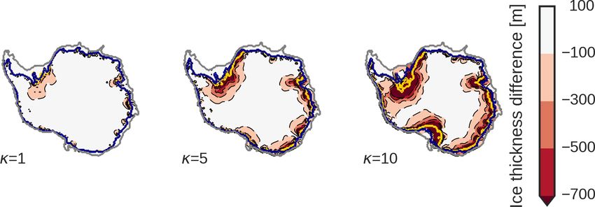
J. Blasco et al.: The Antarctic Ice Sheet response                                                                                 125

                                                                     sponds in a similar manner to the oceanic warming but with
                                                                     less impact. Grounding line migrations and ice discharges are
                                                                     not restricted to the WAIS but also occur in the coastal zones
                                                                     of the EAIS, which goes all along the Amery shelf down to
                                                                     Wilkes Land.
                                                                        The longest ice regrowth periods, corresponding to cool-
                                                                     ing phases, happen between 70 and 60 ka and between 40
                                                                     and 20 ka. During these periods, for medium to low sensi-
Figure 2. Mask used to evaluate grounding line migration. (a) Ice    tivities (up to κ = 7 m a−1 K1 ), the grounding line position
extent after glacial spin-up and (b) PD ice extension. Blue zones    (as indicated by the MZO) advances close to its LGM value,
are model grid cells with grounded ice in marine zones. Grey zones   whereas for high oceanic sensitivities the maximum MZO
are model grid cells without grounded ice in marine zones but the    value reached decreases with increasing κ, indicating the
underlying bathymetry is shallow enough to potentially become        irreversibility typical of hysteresis behavior (Fig. 3c). This
grounded (i.e., marine zones with depths less than 2000 m). The      suggests that the grounding line can readvance up to the con-
thick black line indicates the grounding line position.              tinental shelf break if the oceanic forcing is suppressed long
                                                                     enough, which is not the case for large κ.
                                                                        We further assess what determines the amplitude of ice
present-day (PD) values (Fig. 2b), the grounding line posi-          discharges between 75 and 15 ka (Fig. 7a). During this time
tion has retreated beyond its PD limit. Finally, if MZO = 0,         period we find six significant ice discharge events in response
the grounding line has entirely retreated up to the land with        to enhanced submarine melting phases, marked with grey
its bedrock fully above sea level (i.e., marine zones disap-         shading. Figure 7b shows the ice-volume loss and its cor-
pear). Figure 3c shows the evolution of the MZO for dif-             responding sea-level contribution with respect to κ for every
ferent oceanic sensitivities. After the spin-up, MZO = 0.73          event. Again, for no ice–ocean interaction (κ = 0 m a−1 K1 )
(Fig. 2a). The grounding line has thus advanced towards the          no ice discharges are found, implying that atmospheric mil-
continental shelf break but shelves like the Pine Island zone        lennial variability alone can not produce sea-level variations
or George Land remain ungrounded (Fig. 1a). For κ = 0 the            in the AIS. As the ice–ocean interaction increases with in-
position of the grounding line does not evolve away from the         creasing κ, not only does the sea-level contribution of ev-
spin-up value. Only when the oceanic forcing is considered           ery event increase, but also a wider spread is found between
do grounding line migrations begin to be appreciable. When           the discharging events, meaning that the sea-level difference
oceanic variability is considered, our modeled AIS reacts at         between the smallest and largest ice discharge increases. Fi-
millennial timescales.                                               nally, what determines the total amount of sea-level rise of an
    Figure 4 illustrates the surface elevation (a) and ice ve-       AIM event is the total heat exchange between ice and ocean
locity (b) for three different oceanic sensitivities (κ =1, 5,       (Fig. 8c). If the amplitude is large, generally major ice dis-
and 10 m a−1 K−1 ) after a typical cold phase (at 61 ka). The        charges will be likely, but if the time interval is too short, then
configuration in the three cases is similar, with an advanced        this will not necessarily be true (Fig. 8a). The same is true for
grounding line with grounded Ronne and Ross embayments.              the AIM event duration: longer periods will have more poten-
The grounding line retreat in the Ross shelf increases with          tial time to discharge ice, but if the warming is smooth, less
increasing κ. Ice streams also penetrate further inland with         melting and ice retreat will happen (Fig. 8b).
increasing κ. Figure 5 illustrates the same fields after an
AIM event (at 57 ka). While the lowest sensitivity case (κ =
1 m a−1 K1 ) shows an extensive ice sheet close to the conti-        4   Discussion
nental shelf break similar to the initial LGM state, as the sen-
sitivity increases (κ = 5 m a−1 K1 ) marine zones such as the        Our experimental design follows the bipolar seesaw mecha-
Ronne ice shelf begin to retreat and velocities increase. For        nism (Crowley, 1992; Stocker and Johnsen, 2003) according
sufficiently high oceanic sensitivities (κ = 10 m a−1 K1 ) the       to which the SO acts as a heat reservoir during millennial-
Ronne and Ross ice shelves experience a substantial retreat          scale AMOC reorganizations. However, the extent to which
during AIM events. In addition, the ice velocity field shows         the SO temperature increases during the slowdown of the
ice streams penetrating further inland with increasing κ. The        AMOC is under debate. Pedro et al. (2018) have argued that
ice thickness difference between these two snapshots high-           the Antarctic Circumpolar Current (ACC) acts as a barrier
lights the particular embayments for which the AIS is dis-           for heat penetration into the SO and that the postulated heat
charging for increasing ice–ocean sensitivities (see Fig. 6).        reservoir is rather provided by the southern subtropical At-
The majority of the ice loss comes from the Ronne shelf as           lantic and transferred to the AIS by the atmosphere; in ad-
it is the most vulnerable zone to oceanic warming. The Ross          dition, oceanic heat transport changes could be compensated
shelf does not experience a substantial ice loss and grounding       for to a large extent by changes in heat transport by the at-
line retreat until κ>=10 m a−1 K1 . The Pine Island zone re-         mosphere and the Pacific Ocean. Changes in SO overturning

www.clim-past.net/15/121/2019/                                                                      Clim. Past, 15, 121–133, 2019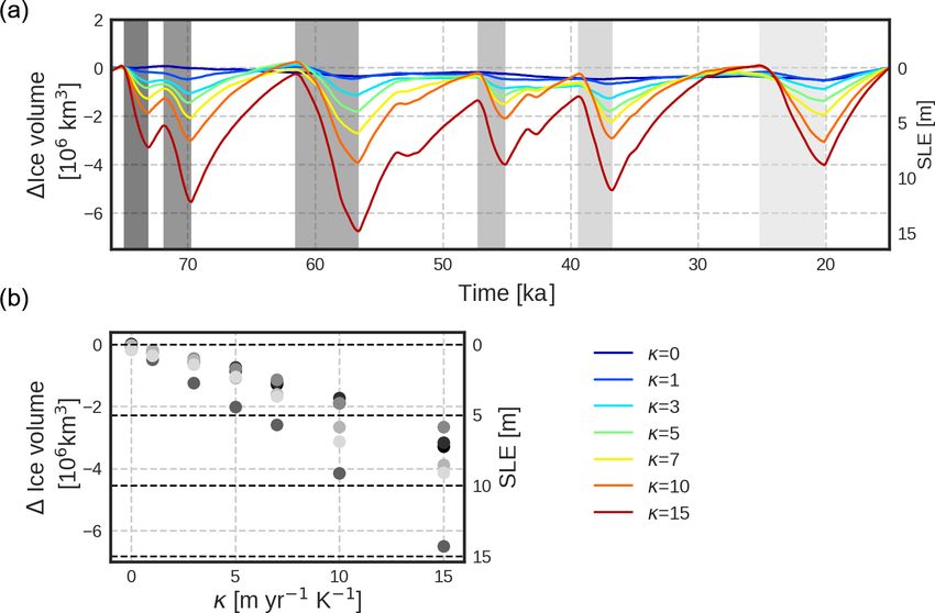
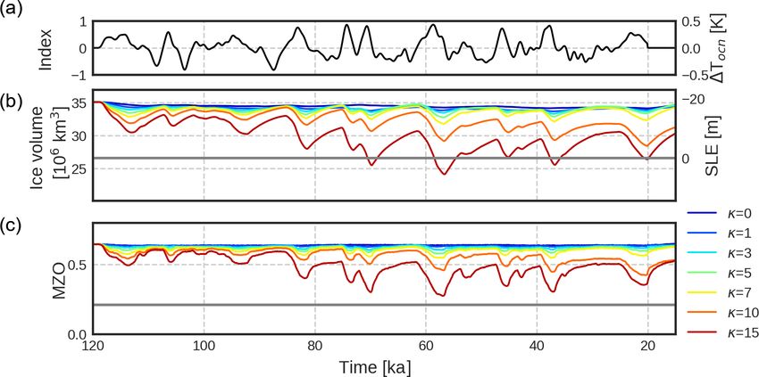
126                                                                                  J. Blasco et al.: The Antarctic Ice Sheet response

Figure 3. (a) Millennial-scale forcing index (β). On the right-hand side the equivalent oceanic temperature anomaly is shown (in K). (b) Ice
volume (in 106 km3 ) and SLE contribution (in m). (c) MZO evolution for different oceanic sensitivities. Colors go from no ice–ocean
interaction (κ = 0 m a−1 K−1 , dark blue) to large oceanic sensitivity (κ = 15 m a−1 K−1 , red). The solid grey line in (b) and (c) indicates the
present-day value of the ice volume and MZO, respectively.

Figure 4. Snapshots of the AIS simulations at a cold phase (61 ka) for three different oceanic sensitivities (κ =1, 5, and 10 m a−1 K−1 ).
(a) Surface elevation (in km). The thick black line indicates the grounding line position, and the thick grey line is the continental shelf break.
(b) Ice velocities (in m a−1 ).

and/or convection can lead to much larger, albeit localized,               construction of the Dome C ice core. This results in an
warming (e.g., Martin et al., 2013, 2014). Positive feedbacks              oceanic temperature anomaly during AIM events of about
resulting from sea-ice and ice-shelf melting could further in-             0.5 K. To our knowledge, there are no reconstructions avail-
crease warming of the subsurface through enhanced stability                able for the SO temperature of high enough temporal resolu-
of the water column (Weber et al., 2014).                                  tion. A lower amplitude for the oceanic temperature anomaly
   For the sake of simplicity we also considered a spatially               in our experimental setup would diminish the effect of the
homogeneous oceanic warming in phase with the atmo-                        millennial-scale oceanic temperature variability. Neverthe-
spheric temperature reconstruction of Dome C. We deduced                   less, our heat transfer coefficient κ can also be interpreted
the oceanic temperature anomaly from the atmospheric re-                   as a weighting parameter of the amount of heat transferred

Clim. Past, 15, 121–133, 2019                                                                             www.clim-past.net/15/121/2019/
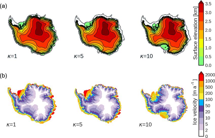
J. Blasco et al.: The Antarctic Ice Sheet response                                                                                           127

Figure 5. Snapshots of the AIS simulations at the end of a warm phase (AIM) event (57 ka) for three different oceanic sensitivities (κ =1,
5, and 10 m a−1 K−1 ). (a) Surface elevation (in km). The thick black line indicates the grounding line position, and the thick grey line is the
continental shelf break. (b) Ice velocities (in m a−1 ).

Figure 6. Ice thickness difference between the AIM and the cold phase (AIM minus cold) for different values of oceanic sensitivity (κ =1, 5,
and 10 m a−1 K−1 ). Zones with an intense red color illustrate a larger ice difference and hence a major ice loss. The thick blue line illustrates
the grounding line position at the cold phase and the thick yellow line the grounding line position at the AIM phase. The thick grey line
illustrates the position of the continental shelf break.

into the SO. However, Buizert et al. (2015) argue that the                    Here we simulated the grounding line migration at mil-
timing difference between the occurrence of DO events in                   lennial timescales for different oceanic sensitivities. We ob-
Greenland ice cores and AIM events provides support for a                  served that at those relatively short timescales, the grounding
slow (oceanic) versus a fast (atmospheric) propagation mech-               line is capable of advancing to its initial state after retreating.
anism from north to south. Hence the main question of how                  Although here we mainly focus on ice-sheet dynamics, we
much the SO warms up during AIM events is unclear and,                     think this variability could be relevant for brine rejection over
again, requires oceanic temperature reconstructions that are               the continental shelf as proposed by Paillard and Parrenin
yet not available.                                                         (2004). The underlying mechanism is that during grounding
   We also found that if the heat flux transfer parameter be-              line advances, brine (salty water released during sea-ice for-
tween ice and ocean is larger than or equal to 10 m a−1 K1                 mation) is pushed out of the continental shelf break. This
then the ice sheet is not able to regrow to its initial state after        salty water descends to the bottom of the ocean, having a
spin-up, neither in volume nor in extent. This highlights the              strong impact on the carbon exchange. If a millennial oscil-
possibility that a heat flux parameter of 10 m a−1 K1 is maybe             lation of the grounding line took place, it could explain the
too large for our ice-sheet model as we know that during the               rise of carbon into the atmosphere, which may be a poten-
LGM the AIS reached its maximum size from reconstruc-                      tial explanation for DO events as well as glacial–interglacial
tions.                                                                     shifts at orbital timescales.

www.clim-past.net/15/121/2019/                                                                               Clim. Past, 15, 121–133, 2019
128                                                                                 J. Blasco et al.: The Antarctic Ice Sheet response

Figure 7. (a) Simulated ice volume anomaly between 75 and 15 ka for different values of oceanic sensitivities. Anomalies are calculated
relative to the state at 15 ka and detrended between 75 and 15 ka. Grey illustrates significant ice discharging events with increasingly darker
grey colors for older events. (b) Scatterplot of the sea-level contribution of every discharging phase with respect to κ.

Figure 8. Ice-volume discharge and SLE contribution of every event against (a) the amplitude of the warming, (b) the duration of the
warming phase, and (c) the integrated warming defined as the peak warming times the duration. Colors represent the different ice–ocean
sensitivities.

Clim. Past, 15, 121–133, 2019                                                                           www.clim-past.net/15/121/2019/
J. Blasco et al.: The Antarctic Ice Sheet response                                                                                    129

   Sea-level reconstructions during MIS-3 show millennial            Author contributions. JB carried out the simulations, analyzed
fluctuations that can reach more than 20 m SLE. These sea-           the results, and wrote the paper. All other authors contributed to de-
level differences are generally attributed to paleo NH ice           signing the simulations, analyzing the results, and writing the paper.
sheets (Arz et al., 2007). Our results highlight the possibil-
ity that a warming of the SO can have a strong impact on
the AIS, producing substantial ice discharges. None of our           Competing interests. The authors declare that they have no con-
results, including those with a high oceanic sensitivity, ex-        flict of interest.
ceeded 20 m SLE. Low sensitivities (κ < 5 m a−1 K1 ) do not
produce discharging events of more than 5 m, which means
                                                                     Acknowledgements. We are grateful to Catherine Ritz for
that NH paleo ice sheets would still be the major contribu-
                                                                     providing the original model GRISLI and to Rubén Banderas for
tors to millennial sea-level fluctuations. For κ > 10 m a−1 K1 ,     helping initially with the model. This work was funded by the Span-
SLE contributions of more than 10 m occur, which would               ish Ministry of Science and Innovation under the project MOCCA
imply a significant Antarctic contribution as well. How-             (Modelling Abrupt Climate Change, grant no. CGL2014-59384-R).
ever, as discussed above, this contribution (and for larger          Ilaria Tabone is funded by the Spanish National Programme for the
oceanic sensitivities) seems unrealistic as our model does           Promotion of Talent and its Employability (grant no. BES-2015-
not support a regrowth of the AIS to the continental shelf           074097). Alexander Robinson is funded by the Ramón y Cajal
break under LGM climate conditions. Intermediate values              Programme of the Spanish Ministry for Science, Innovation and
(κ = 7 m a−1 K1 ) lead to discharges of around 6 m SLE. A            Universities. All of these simulations were performed in EOLO, the
non-negligible Antarctic contribution to sea-level changes at        HPC of Climate Change of the International Campus of Excellence
millennial timescales during the LGP will have an impact on          of Moncloa, funded by MECD and MICINN.
reconstructing the size of other paleo ice sheets.
                                                                     Edited by: Steven Phipps
                                                                     Reviewed by: two anonymous referees

5   Conclusions
                                                                     References
We have investigated the response of the AIS to millennial-
scale climate variability and, in particular, its response to dif-   Alvarez-Solas, J., Charbit, S., Ramstein, G., Paillard, D., Du-
ferent oceanic sensitivities using a hybrid, three-dimensional,        mas, C., Ritz, C., and Roche, D. M.: Millennial-scale os-
thermomechanical ice-sheet model. The model is forced us-              cillations in the Southern Ocean in response to atmo-
ing a method that has already been tested (Banderas et al.,            spheric CO 2 increase, Global Planet. Change, 76, 128–136,
2018) and is provided by an improved subglacial melting                https://doi.org/10.1016/j.gloplacha.2010.12.004, 2011.
routine. Because SO temperature reconstructions are not              Alvarez-Solas, J., Robinson, A., Montoya, M., and Ritz, C.: Ice-
available we assumed that oceanic temperatures covary with             berg discharges of the last glacial period driven by oceanic cir-
atmospheric temperature variations at millennial timescales            culation changes, P. Natl. Acad. Sci. USA, 110, 16350–16354,
based on Stocker and Johnsen (2003). Our simulations sug-              https://doi.org/10.1073/pnas.1306622110, 2013.
                                                                     Alvarez-Solas, J., Banderas, R., Robinson, A., and Montoya, M.:
gest that, contrary to the idea that the AIS is a slow reac-
                                                                       Oceanic forcing of the Eurasian Ice Sheet on millennial time
tive ice sheet, it could be more reactive to millennial-scale          scales during the Last Glacial Period, Clim. Past Discuss.,
climate variabilities than previously thought. We found that           https://doi.org/10.5194/cp-2017-143, 2017.
whereas atmospheric millennial-scale variability had no ap-          Anderson, J. B., Shipp, S. S., Lowe, A. L., Wellner, J. S., and
preciable impact on the AIS, SO warming could produce                  Mosola, A. B.: The Antarctic Ice Sheet during the Last Glacial
episodes of ice discharge, leading to substantial sea-level rise       Maximum and its subsequent retreat history: a review, Qua-
and grounding line migration. Although this timescale may              ternary Sci. Rev., 21, 49–70, https://doi.org/10.1016/S0277-
seem short for such a large ice sheet, our simulations show,           3791(01)00083-X, 2002.
in the range of realistic values for oceanic sensitivities, that     Andrews, J. T. and Voelker, A. H.: “Heinrich Events” (&
considerable grounding line retreat in the Ronne, Ross, and            sediments): A history of terminology and recommenda-
Wilkes Land embayment, as well as sea-level discharge of               tions for future usage, Quaternary Sci. Rev., 187, 31–40,
                                                                       https://doi.org/10.1016/j.quascirev.2018.03.017, 2018.
around 6 m SLE at millennial timescales, can occur. Our re-
                                                                     Arz, H. W., Lamy, F., Ganopolski, A., Nowaczyk,
sults highlight the possibility that, via the bipolar seesaw, a
                                                                       N., and Pätzold, J.: Dominant Northern Hemisphere
slowdown of the AMOC could have accumulated more heat                  climate     control   over     millennial-scale    glacial   sea-
in the Southern Ocean, resulting in significant sea-level rise         level variability, Quaternary Sci. Rev., 26, 312–321,
produced by the AIS on millennial timescales.                          https://doi.org/10.1016/j.quascirev.2006.07.016, 2007.
                                                                     Augustin, L., Barbante, C., Barnes, P. R., Barnola, J. M., Bigler,
                                                                       M., Castellano, E., Cattani, O., Chappellaz, J., Dahl-Jensen, D.,
Code and data availability. GRISLI-UCM code and the ana-               Delmonte, B., Dreyfus, G., Durand, G., Falourd, S., Fischer,
lyzed data are available from the authors upon request.                H., Fluckiger, J., Hansson, M. E., Huybrechts, P., Jugie, G.,

www.clim-past.net/15/121/2019/                                                                        Clim. Past, 15, 121–133, 2019
130 J. Blasco et al.: The Antarctic Ice Sheet response Johnsen, S. J., Jouzel, J., Kaufmann, P., Kipfstuhl, J., Lam- Böhm, E., Lippold, J., Gutjahr, M., Frank, M., Blaser, P., Antz, bert, F., Lipenkov, V. Y., Littot, G. C., Longinelli, A., Lor- B., Fohlmeister, J., Frank, N., Andersen, M., and Deininger, rain, R., Maggi, V., Masson-Delmotte, V., Miller, H., Mul- M.: Strong and deep Atlantic meridional overturning cir- vaney, R., Oerlemans, J., Oerter, H., Orombelli, G., Parrenin, culation during the last glacial cycle, Nature, 517, 73–76, F., Peel, D. A., Petit, J.-R., Raynaud, D., Ritz, C., Ruth, U., https://doi.org/10.1038/nature14059, 2015. Schwander, J., Siegenthaler, U., Souchez, R., Stauffer, B., Stef- Buizert, C., Adrian, B., Ahn, J., Albert, M., Alley, R. B., Baggen- fensen, J. P., Stenni, B., Stocker, T. F., Tabacco, I. E., Udisti, stos, D., Bauska, T. K., Bay, R. C., Bencivengo, B. B., Bent- R., van der Wal, R. S., van den Broeke, M., Weiss, J., Will- ley, C. R., Brook, E. J., Chellman, N. J., Clow, G. D., Cole- helms, F., Winther, J.-G., Wolff, E. W., and Zucchelli, M.: Eight Dai, J., Conway, H., Cravens, E., Cuffey, K. M., Dunbar, N. glacial cycles from an Antarctic ice core, Nature, 429, 623–628, W., Edwards, J. S., Fegyveresi, J. M., Ferris, D. G., Fitzpatrick, https://doi.org/10.1038/nature02599, 2004. J. J., Fudge, T. J., Gibson, C. J., Gkinis, V., Goetz, J. J., Gre- Bakker, A. M., Wong, T. E., Ruckert, K. L., and Keller, K.: gory, S., Hargreaves, G. M., Iverson, N., Johnson, J. A., Jones, T. Sea-level projections representing the deeply uncertain contri- R., Kalk, M. L., Kippenhan, M. J., Koffman, B. G., Kreutz, K., bution of the West Antarctic ice sheet, Sci. Rep., 7, 3880, Kuhl, T. W., Lebar, D. A., Lee, J. E., Marcott, S. A., Markle, B. https://doi.org/10.1038/s41598-017-04134-5, 2017a. R., Maselli, O. J., McConnell, J. R., McGwire, K. C., Mitchell, Bakker, A. M. R., Louchard, D., and Keller, K.: Sources and impli- L. E., Mortensen, N. B., Neff, P. D., Nishiizumi, K., Nunn, R. cations of deep uncertainties surrounding sea-level projections, M., Orsi, A. J., Pasteris, D. R., Pedro, J. B., Pettit, E. C., Price, Climatic Change, 140, 339–347, https://doi.org/10.1007/s10584- P. B., Priscu, J. C., Rhodes, R. H., Rosen, J. L., Schauer, A. 016-1864-1, 2017b. J., Schoenemann, S. W., Sendelbach, P. J., Severinghaus, J. P., Bamber, J. L., Riva, R. E., Vermeersen, B. L., and LeBrocq, Shturmakov, A. J., Sigl, M., Slawny, K. R., Souney, J. M., Sow- A. M.: Reassessment of the potential sea-level rise from a col- ers, T. A., Spencer, M. K., Steig, E. J., Taylor, K. C., Twickler, lapse of the West Antarctic Ice Sheet, Science, 324, 901–903, M. S., Vaughn, B. H., Voigt, D. E., Waddington, E. D., Welten, https://doi.org/10.1126/science.1169335, 2009. K. C., Wendricks, A. W., White, J. W. C., Winstrup, M., Wong, Banderas, R., Alvarez-Solas, J., Robinson, A., and Montoya, M.: A G. J., and Woodruf, T. E.: Precise interpolar phasing of abrupt new approach for simulating the paleo-evolution of the North- climate change during the last ice age, Nature, 520, 661–665, ern Hemisphere ice sheets, Geosci. Model Dev., 11, 2299–2314, https://doi.org/10.1038/nature14401, 2015. https://doi.org/10.5194/gmd-11-2299-2018, 2018. Collins, M., Knutti, R., Arblaster, J. M., Dufresne, J. L., Fichefet, T., Barker, S., Chen, J., Gong, X., Jonkers, L., Knorr, G., and Thornal- Friedlingstein, P., Gao, X., Gutowski, W. J., Johns, T., Krinner, ley, D.: Icebergs not the trigger for North Atlantic cold events, G., Shongwe, M., Tebaldi, C., Weaver, A. J., and Wehner, M.: Nature, 520, 333–336, https://doi.org/10.1038/nature14330, Climate Change 2013: The Physical Science Basis. Contribution 2015. of Working Group I to the Fifth Assessment Report of the Inter- Beckmann, A. and Goosse, H.: A parameterization of ice shelf– governmental Panel on Climate Change, edited by: Stocker, T., ocean interaction for climate models, Ocean Model., 5, 157–170, Qin, D., Plattner, G., Tignor, M. M. B., Allen, S. K., Boschung, https://doi.org/10.1016/S1463-5003(02)00019-7, 2003. J., Nauels, A., Xia, Y., Bex, V., and Midgley, P. M., Cambridge Bentley, M. J., Cofaigh, C. O., Anderson, J. B., Conway, H., Univ. Press, 1029–1136, 2013. Davies, B., Graham, A. G., Hillenbrand, C.-D., Hodgson, D. Crowley, T. J.: North Atlantic deep water cools the A., Jamieson, S. S., Larter, R. D., Mackintosh, A., Smith, J. A., Southern Hemisphere, Paleoceanography, 7, 489–497, Verleyen, E., Ackert, R. P., Bart, P. J., Berg, S., Brunstein, D., https://doi.org/10.1029/92PA01058, 1992. Canals, M., Colhoun, E. A., Crosta, X., Dickens, W. A., Do- Dansgaard, W., Johnsen, S., Clausen, H., Dahl-Jensen, D., Gunde- mack, E., Dowdeswell, J. A., Dunbar, R., Ehrmann, W., Evans, strup, N., Hammer, C., Hvidberg, C., Steffensen, J., Sveinbjörns- J., Favier, V., Fink, D., Fogwill, C. J., Glasser, N. F., Gohl, dottir, A., Jouzel, J., and Bond, G.: Evidence for general instabil- K., Golledge, N. R., Goodwin, I., Gore, D. B., Greenwood, S. ity of past climate from a 250-kyr ice-core record, Nature, 364, L., Hall, B. L., Hall, K., Hedding, D. W., Hein, A. S., Hock- 218–20, https://doi.org/10.1038/364218a0, 1993. ing, E. P., Jakobsson, M., Johnson, J. S., Jomelli, V., Jones, DeConto, R. M. and Pollard, D.: Contribution of Antarctica R. S., Klages, J. P., Kristoffersen, Y., Kuhn, G., Leventer, A., to past and future sea-level rise, Nature, 531, 591–597, Licht, K., Lilly, K., Lindow, J., Livingstone, S. J., Massé, G., https://doi.org/10.1038/nature17145, 2016. McGlone, M. S., McKay, R. M., Melles, M., Miura, H., Mul- Dee, D. P., Uppala, S., Simmons, A., Berrisford, P., Poli, P., vaney, R., Nela, W., Nitsche, F. O., O’Brien, P. E., Post, A. Kobayashi, S., Andrae, U., Balmaseda, M., Balsamo, G., Bauer, L., Roberts, S. J., Saunders, K. M., Selkirk, P. M., Simms, A. P., Bechtold, P., Beljaars, A. C. M., van de Berg, L., Bidlot, J., R., Spiegel, C., Stolldorf, T. D., Sugden, D. E., van der Put- Bormann, N., Delsol, C., Dragani, R., Fuentes, M., Geer, A. J., ten, N., van Ommen, T., Verfaillie, D., Vyverman, W., Wagner, Haimberger, L., Healy, S. B., Hersbach, H., Holm, E. V., Isak- B., White, D. A., Witus, A. E., and Zwartz, D.: A community- sen, L., Kallberg, P., Kohler, M., Matricardi, M., McNally, A. P., based geological reconstruction of Antarctic Ice Sheet deglacia- Monge Sanz, B. M., Morcrette, J. J., Park, B. K., Peubey, C., tion since the Last Glacial Maximum, Quaternary Sci. Rev., 100, de Rosnay, P., Tavolato, C., Thépaut, J. N., and Vitart, F.: The 1–9, https://doi.org/10.1016/j.quascirev.2014.06.025, 2014. ERA-Interim reanalysis: Configuration and performance of the Blunier, T. and Brook, E. J.: Timing of millennial-scale data assimilation system, Q. J. Roy. Meteor. Soc., 137, 553–597, climate change in Antarctica and Greenland dur- https://doi.org/10.1002/qj.828, 2011. ing the last glacial period, Science, 291, 109–112, Denton, G. H. and Hughes, T. J.: Reconstructing the Antarctic https://doi.org/10.1126/science.291.5501.109, 2001. ice sheet at the Last Glacial Maximum, Quaternary Sci. Rev., Clim. Past, 15, 121–133, 2019 www.clim-past.net/15/121/2019/
J. Blasco et al.: The Antarctic Ice Sheet response                                                                                            131

   21, 193–202, https://doi.org/10.1016/S0277-3791(01)00090-7,                 Geophys., 42, RG1005, https://doi.org/10.1029/2003RG000128,
   2002.                                                                       2004.
EPICA Community Members: One-to-one coupling of glacial cli-                Henry, L., McManus, J. F., Curry, W. B., Roberts, N. L., Piotrowski,
   mate variability in Greenland and Antarctica, Nature, 444, 195–             A. M., and Keigwin, L. D.: North Atlantic ocean circulation and
   198, https://doi.org/10.1038/nature05301, 2006.                             abrupt climate change during the last glaciation, Science, 353,
Favier, L., Durand, G., Cornford, S. L., Gudmundsson, G. H.,                   470–474, https://doi.org/10.1126/science.aaf5529, 2016.
   Gagliardini, O., Gillet-Chaulet, F., Zwinger, T., Payne, A., and         Hillenbrand, C.-D., Melles, M., Kuhn, G., and Larter, R. D.: Ma-
   Le Brocq, A. M.: Retreat of Pine Island Glacier controlled by               rine geological constraints for the grounding-line position of
   marine ice-sheet instability, Nat. Clim. Change, 4, 117–121,                the Antarctic Ice Sheet on the southern Weddell Sea shelf at
   https://doi.org/10.1038/nclimate2094, 2014.                                 the Last Glacial Maximum, Quaternary Sci. Rev., 32, 25–47,
Feldmann, J. and Levermann, A.: Collapse of the West Antarc-                   https://doi.org/10.1016/j.quascirev.2011.11.017, 2012.
   tic Ice Sheet after local destabilization of the Amund-                  Hutter, K.: Theoretical glaciology; material science of ice and
   sen Basin, P. Natl. Acad. Sci. USA, 112, 14191–14196,                       the mechanics of glaciers and ice sheets, D. Reidel Publishing
   https://doi.org/10.1073/pnas.1512482112, 2015.                              Co./Tokyo, Terra Scintific Publishing Co, 1983.
Fretwell, P., Pritchard, H. D., Vaughan, D. G., Bamber, J. L., Bar-         Jacobs, S. S., Jenkins, A., Giulivi, C. F., and Dutrieux,
   rand, N. E., Bell, R., Bianchi, C., Bingham, R. G., Blanken-                P.: Stronger ocean circulation and increased melting under
   ship, D. D., Casassa, G., Catania, G., Callens, D., Conway, H.,             Pine Island Glacier ice shelf, Nat. Geosci., 4, 519–523,
   Cook, A. J., Corr, H. F. J., Damaske, D., Damm, V., Ferracci-               https://doi.org/10.1038/ngeo1188, 2011.
   oli, F., Forsberg, R., Fujita, S., Gim, Y., Gogineni, P., Griggs,        Jouzel, J. and Masson-Delmotte, V.: EPICA Dome C Ice Core
   J. A., Hindmarsh, R. C. A., Holmlund, P., Holt, J. W., Jacobel,             800KYr deuterium data and temperature estimates, 2007.
   R. W., Jenkins, A., Jokat, W., Jordan, T., King, E. C., Kohler,          Kim, S., Yoo, K.-C., Lee, J. I., Lee, M. K., Kim, K., Yoon,
   J., Krabill, W., Riger-Kusk, M., Langley, K. A., Leitchenkov,               H. I., and Moon, H. S.: Relationship between magnetic sus-
   G., Leuschen, C., Luyendyk, B. P., Matsuoka, K., Mouginot,                  ceptibility and sediment grain size since the last glacial
   J., Nitsche, F. O., Nogi, Y., Nost, O. A., Popov, S. V., Rignot,            period in the Southern Ocean off the northern Antarc-
   E., Rippin, D. M., Rivera, A., Roberts, J., Ross, N., Siegert,              tic Peninsula–Linkages between the cryosphere and atmo-
   M. J., Smith, A. M., Steinhage, D., Studinger, M., Sun, B.,                 spheric circulation, Palaeogeogr. Palaeocl., 505, 359–370,
   Tinto, B. K., Welch, B. C., Wilson, D., Young, D. A., Xiangbin,             https://doi.org/10.1016/j.palaeo.2018.06.016, 2018.
   C., and Zirizzotti, A.: Bedmap2: improved ice bed, surface and           Kusahara, K., Sato, T., Oka, A., Obase, T., Greve, R., Abe-Ouchi,
   thickness datasets for Antarctica, The Cryosphere, 7, 375–393,              A., and Hasumi, H.: Modelling the Antarctic marine cryosphere
   https://doi.org/10.5194/tc-7-375-2013, 2013.                                at the Last Glacial Maximum, Ann. Glaciol., 56, 425–435,
Frigola, J., Canals, M., Cacho, I., Moreno, A., Sierro, F. J., Flores, J.      https://doi.org/10.3189/2015AoG69A792, 2015.
   A., Berné, S., Jouet, G., Dennielou, B., Herrera, G., Pasqual, C.,       Liu, J., Milne, G. A., Kopp, R. E., Clark, P. U., and Shen-
   Grimalt, J. O., Galavazi, M., and Schneider, R.: A 500 kyr record           nan, I.: Sea-level constraints on the amplitude and source dis-
   of global sea-level oscillations in the Gulf of Lion, Mediterranean         tribution of Meltwater Pulse 1A, Nat. Geosci., 9, 130–134,
   Sea: new insights into MIS 3 sea-level variability, Clim. Past, 8,          https://doi.org/10.1038/NGEO2616, 2016.
   1067–1077, https://doi.org/10.5194/cp-8-1067-2012, 2012.                 MacAyeal, D. R.: Large-scale ice flow over a viscous
Fürst, J. J., Durand, G., Gillet-Chaulet, F., Tavard, L., Rankl,               basal sediment: Theory and application to ice stream
   M., Braun, M., and Gagliardini, O.: The safety band of                      B, Antarctica, J. Geophys. Res., 94, 4071–4087,
   Antarctic ice shelves, Nat. Clim. Change, 6, 479–482,                       https://doi.org/10.1029/JB094iB04p04071, 1989.
   https://doi.org/10.1038/nclimate2912, 2016.                              Marcott, S. A., Shakun, J. D., Clark, P. U., and Mix,
Ganopolski, A. and Rahmstorf, S.: Rapid changes of glacial cli-                A. C.: A reconstruction of regional and global tempera-
   mate simulated in a coupled climate model, Nature, 409, 153–                ture for the past 11,300 years, Science, 339, 1198–1201,
   158, https://doi.org/10.1038/35051500, 2001.                                https://doi.org/10.1126/science.1228026, 2013.
Ganopolski, A., Calov, R., and Claussen, M.: Simulation of                  Martin, T., Park, W., and Latif, M.: Multi-centennial variability con-
   the last glacial cycle with a coupled climate ice-sheet                     trolled by Southern Ocean convection in the Kiel Climate Model,
   model of intermediate complexity, Clim. Past, 6, 229–244,                   Clim. Dynam., 40, 2005–2022, https://doi.org/10.1007/s00382-
   https://doi.org/10.5194/cp-6-229-2010, 2010.                                012-1586-7, 2013.
Golledge, N. R., Kowalewski, D. E., Naish, T. R., Levy, R. H.,              Martin, T., Steele, M., and Zhang, J.: Seasonality and
   Fogwill, C. J., and Gasson, E. G.: The multi-millennial Antarc-             long-term trend of Arctic Ocean surface stress in a
   tic commitment to future sea-level rise, Nature, 526, 421–425,              model, J. Geophys. Res.-Oceans, 119, 1723–1738,
   https://doi.org/10.1038/nature15706, 2015.                                  https://doi.org/10.1002/2013JC009425, 2014.
Grant, K., Rohling, E., Bar-Matthews, M., Ayalon, A., Medina-               Martín-Español, A., Zammit-Mangion, A., Clarke, P. J., Flament,
   Elizalde, M., Ramsey, C. B., Satow, C., and Roberts, A.:                    T., Helm, V., King, M. A., Luthcke, S. B., Petrie, E., Rémy, F.,
   Rapid coupling between ice volume and polar tempera-                        Schön, N., Wouters, B., and Bamber, J. L.: Spatial and tempo-
   ture over the past 150,000 years, Nature, 491, 744–747,                     ral Antarctic Ice Sheet mass trends, glacio-isostatic adjustment,
   https://doi.org/10.1038/nature11593, 2012.                                  and surface processes from a joint inversion of satellite altimeter,
Hemming, S. R.: Heinrich events: Massive late Pleistocene detritus             gravity, and GPS data, J. Geophys. Res.-Earth, 121, 182–200,
   layers of the North Atlantic and their global climate imprint, Rev.         https://doi.org/10.1002/2015JF003550, 2016.

www.clim-past.net/15/121/2019/                                                                               Clim. Past, 15, 121–133, 2019
132                                                                               J. Blasco et al.: The Antarctic Ice Sheet response

McManus, J. F., Francois, R., Gherardi, J.-M., Keigwin, L. D.,             Res. Lett., 31, L18401, https://doi.org/10.1029/2004GL020697,
  and Brown-Leger, S.: Collapse and rapid resumption of Atlantic           2004.
  meridional circulation linked to deglacial climate changes, Na-       Rignot, E., Jacobs, S., Mouginot, J., and Scheuchl, B.: Ice-
  ture, 428, 834–837, https://doi.org/10.1038/nature02494, 2004.           shelf melting around Antarctica, Science, 341, 266–270,
Mercer, J. H.: West Antarctic ice sheet and CO2 green-                     https://doi.org/10.1126/science.1235798, 2013.
  house effect- A threat of disaster, Nature, 271, 321–325,             Ritz, C., Rommelaere, V., and Dumas, C.: Modeling the evolution of
  https://doi.org/10.1038/271321a0, 1978.                                  Antarctic ice sheet over the last 420,000 years: Implications for
Montoya, M. and Levermann, A.: Surface wind-stress threshold for           altitude changes in the Vostok region, J. Geophys. Res.-Atmos.,
  glacial Atlantic overturning, Geophys. Res. Lett., 35, L03608,           106, 31943–31964, https://doi.org/10.1029/2001JD900232,
  https://doi.org/10.1029/2007GL032560, 2008.                              2001.
Nicholls, R. J. and Cazenave, A.: Sea-level rise and its                Rohling, E., Foster, G. L., Grant, K., Marino, G., Roberts, A.,
  impact on coastal zones, Science, 328, 1517–1520,                        Tamisiea, M. E., and Williams, F.: Sea-level and deep-sea-
  https://doi.org/10.1126/science.1185782, 2010.                           temperature variability over the past 5.3 million years, Nature,
Paillard, D. and Parrenin, F.: The Antarctic ice sheet and the trig-       508, 477–482, https://doi.org/10.1038/nature13230, 2014.
  gering of deglaciations, Earth Planet. Sc. Lett., 227, 263–271,       Rohling, E. J., Grant, K., Bolshaw, M., Roberts, A., Siddall, M.,
  https://doi.org/10.1016/j.epsl.2004.08.023, 2004.                        Hemleben, C., and Kucera, M.: Antarctic temperature and global
Paolo, F. S., Fricker, H. A., and Padman, L.: Volume loss from             sea level closely coupled over the past five glacial cycles, Nat.
  Antarctic ice shelves is accelerating, Science, 348, 327–331,            Geosci., 2, 500–504, https://doi.org/10.1038/ngeo557, 2009.
  https://doi.org/10.1126/science.aaa0940, 2015.                        Ruth, U., Barnola, J.-M., Beer, J., Bigler, M., Blunier, T., Castel-
Pattyn, F.: Sea-level response to melting of Antarctic ice shelves on      lano, E., Fischer, H., Fundel, F., Huybrechts, P., Kaufmann, P.,
  multi-centennial timescales with the fast Elementary Thermome-           Kipfstuhl, S., Lambrecht, A., Morganti, A., Oerter, H., Parrenin,
  chanical Ice Sheet model (f.ETISh v1.0), The Cryosphere, 11,             F., Rybak, O., Severi, M., Udisti, R., Wilhelms, F., and Wolff,
  1851–1878, https://doi.org/10.5194/tc-11-1851-2017, 2017.                E.: “EDML1”: a chronology for the EPICA deep ice core from
Pedro, J. B., Jochum, M., Buizert, C., He, F., Barker, S., and Ras-        Dronning Maud Land, Antarctica, over the last 150 000 years,
  mussen, S. O.: Beyond the bipolar seesaw: Toward a process un-           Clim. Past, 3, 475–484, https://doi.org/10.5194/cp-3-475-2007,
  derstanding of interhemispheric coupling, Quaternary Sci. Rev.,          2007.
  192, 27–46, https://doi.org/10.1016/j.quascirev.2018.05.005,          Schaffer, J., Timmermann, R., Arndt, J. E., Kristensen, S. S.,
  2018.                                                                    Mayer, C., Morlighem, M., and Steinhage, D.: A global, high-
Petit, J.-R., Jouzel, J., Raynaud, D., Barkov, N. I., Barnola, J.-M.,      resolution data set of ice sheet topography, cavity geome-
  Basile, I., Bender, M., Chappellaz, J., Davis, M., Delaygue, G.,         try, and ocean bathymetry, Earth Syst. Sci. Data, 8, 543–557,
  Delmotte, M., Kotlyakov, V. M., Legrand, M., Lipenkov, V. Y.,            https://doi.org/10.5194/essd-8-543-2016, 2016.
  Lorius, C., Pépin, L., Ritz, C., Saltzman, E., and Stievenard,        Schoof, C.: Ice sheet grounding line dynamics: Steady states, sta-
  M.: Climate and atmospheric history of the past 420,000 years            bility, and hysteresis, J. Geophys. Res.-Earth, 112, F03S28,
  from the Vostok ice core, Antarctica, Nature, 399, 429–436,              https://doi.org/10.1029/2006JF000664, 2007.
  https://doi.org/10.1038/20859, 1999.                                  Shaffer, G., Olsen, S. M., and Bjerrum, C. J.: Ocean subsurface
Peyaud, V., Ritz, C., and Krinner, G.: Modelling the Early                 warming as a mechanism for coupling Dansgaard-Oeschger cli-
  Weichselian Eurasian Ice Sheets: role of ice shelves and                 mate cycles and ice-rafting events, Geophys. Res. Lett., 31,
  influence of ice-dammed lakes, Clim. Past, 3, 375–386,                   L24202, https://doi.org/10.1029/2004GL020968, 2004.
  https://doi.org/10.5194/cp-3-375-2007, 2007.                          Shapiro, N. M. and Ritzwoller, M. H.: Inferring surface heat flux
Philippon, G., Ramstein, G., Charbit, S., Kageyama, M., Ritz, C.,          distributions guided by a global seismic model: particular ap-
  and Dumas, C.: Evolution of the Antarctic ice sheet throughout           plication to Antarctica, Earth Planet. Sc. Lett., 223, 213–224,
  the last deglaciation: a study with a new coupled climate-north          https://doi.org/10.1016/j.epsl.2004.04.011, 2004.
  and south hemisphere ice sheet model, Earth Planet. Sc. Lett.,        Shepherd, A., Ivins, E., Rignot, E., Smith, B., van den Broeke, M.,
  248, 750–758, https://doi.org/10.1016/j.epsl.2006.06.017, 2006.          Velicogna, I., Whitehouse, P., Briggs, K., Joughin, I., Krinner, G.,
Pollard, D. and DeConto, R. M.: Modelling West Antarctic ice sheet         Nowicki, S., Payne, T., Scambos, T., Schlegel, N., A, G., Agosta,
  growth and collapse through the past five million years, Nature,         C., Ahlstrøm, A., Babonis, G., Barletta, V., Blazquez, A., Bonin,
  458, 329–332, https://doi.org/10.1038/nature07809, 2009.                 J., Csatho, B., Cullather, R., Felikson, D., Fettweis, X., Fors-
Rahmstorf, S.: Ocean circulation and climate dur-                          berg, R., Gallee, H., Gardner, A., Gilbert, L., Groh, A., Gunter,
  ing the past 120,000 years, Nature, 419, 207–214,                        B., Hanna, E., Harig, C., Helm, V., Horvath, A., Horwath, M.,
  https://doi.org/10.1038/nature01090, 2002.                               Khan, S., Kjeldsen, K. K., Konrad, H., Langen, P., Lecavalier,
Reeh, N.: Parameterization of melt rate and surface temperature on         B., Loomis, B., Luthcke, S., McMillan, M., Melini, D., Mernild,
  the Greenland ice sheet, J. Geophys. Res.-Sol. Ea., 59, 113–128,         S., Mohajerani, Y., Moore, P., Mouginot, J., Moyano, G., Muir,
  1989.                                                                    A., Nagler, T., Nield, G., Nilsson, J., Noel, B., Otosaka, I., Pattle,
Rignot, E. and Jacobs, S. S.: Rapid bottom melting widespread near         M. E., Peltier, W. R., Pie, N., Rietbroek, R., Rott, H., Sandberg-
  Antarctic ice sheet grounding lines, Science, 296, 2020–2023,            Sørensen, L., Sasgen, I., Save, H., Scheuchl, B., Schrama, E.,
  https://doi.org/10.1126/science.1070942, 2002.                           Schröder, L., Seo, K.-W., Simonsen, S., Slater, T., Spada, G.,
Rignot, E., Casassa, G., Gogineni, P., Krabill, W., Rivera, A. U.,         Sutterley, T., Talpe, M., Tarasov, L., van de Berg, W. J., van der
  and Thomas, R.: Accelerated ice discharge from the Antarctic             Wal, W., van Wessem, M., Vishwakarma, B. D., Wiese, D., and
  Peninsula following the collapse of Larsen B ice shelf, Geophys.         Wouters, B.: Mass balance of the Antarctic Ice Sheet from 1992

Clim. Past, 15, 121–133, 2019                                                                           www.clim-past.net/15/121/2019/
You can also read