Resolving the ambiguous direction of arrival of weak meteor radar trail echoes
←
→
Page content transcription
If your browser does not render page correctly, please read the page content below
Atmos. Meas. Tech., 14, 3583–3596, 2021
https://doi.org/10.5194/amt-14-3583-2021
© Author(s) 2021. This work is distributed under
the Creative Commons Attribution 4.0 License.

Resolving the ambiguous direction of arrival of
weak meteor radar trail echoes
Daniel Kastinen1,2 , Johan Kero1 , Alexander Kozlovsky3 , and Mark Lester4
1 Swedish Institute of Space Physics (IRF), Box 812, 98128 Kiruna, Sweden
2 Department of Physics, Umeå University, 90187 Umeå, Sweden
3 Sodankylä Geophysical Observatory, Sodankylä, Finland
4 Department of Physics and Astronomy, University of Leicester, Leicester, United Kingdom

Correspondence: Daniel Kastinen (daniel.kastinen@irf.se)

Received: 11 June 2020 – Discussion started: 18 September 2020
Revised: 20 March 2021 – Accepted: 22 March 2021 – Published: 19 May 2021

Abstract. Meteor phenomena cause ionized plasmas that can         results are compared to Bayesian inference using the DMC
be roughly divided into two distinctly different regimes: a       simulations and the standard SkiYMET data products. In the
dense and transient plasma region co-moving with the ablat-       examined data set, ∼ 13 % of the events were indicated as
ing meteoroid and a trail of diffusing plasma left in the at-     ambiguous. Out of these, ∼ 13 % contained anomalous sig-
mosphere and moving with the neutral wind. Interferometric        nals. In ∼ 95 % of all ambiguous cases with a nominal sig-
radar systems are used to observe the meteor trails and de-       nal, the three methods found one and the same output DOA,
termine their positions and drift velocities. Depending on the    which was also listed as one of the ambiguous possibilities in
spatial configuration of the receiving antennas and their in-     the SkiYMET analysis. In all unambiguous cases, the results
dividual gain patterns, the voltage response can be the same      from all methods concurred.
for several different plane wave directions of arrival (DOAs),
thereby making it impossible to determine the correct direc-
tion. A low signal-to-noise ratio (SNR) can create the same       1   Introduction
effect probabilistically even if the system contains no the-
oretical ambiguities. Such is the case for the standard me-       Every day the Earth’s atmosphere is bombarded by bil-
teor trail echo data products of the Sodankylä Geophysical        lions of dust-sized particles and larger pieces of material
Observatory SKiYMET all-sky interferometric meteor radar.         from space. In doing so these objects, called meteoroids,
Meteor trails drift slowly enough in the atmosphere and al-       ablate and produce phenomena called meteors (Ceplecha
low for temporal integration, while meteor head echo targets      et al., 1998). These phenomena are commonly seen as vis-
move too fast. Temporal integration is a common method to         ible streaks of light in the night sky.
increase the SNR of radar signals. For meteor head echoes,           Meteor phenomena cause ionized plasmas that can be
we instead propose to use direct Monte Carlo (DMC) simula-        roughly divided into two distinctly different regimes: a dense
tions to validate DOA measurements. We have implemented           and transient plasma region co-moving with the ablating me-
two separate temporal integration methods and applied them        teoroid and a trail of diffusing plasma left in the atmosphere
to 2222 events measured by the Sodankylä meteor radar to          and moving with the neutral wind. Both of these plasmas re-
simultaneously test the usefulness of such DMC simulations        flect radio waves (Lovell et al., 1947). When measured with
on cases where temporal integration is possible, validate the     a radar, they cause so-called meteor head and meteor trail
temporal integration methods, and resolve the ambiguous           echoes (McKinley, 1961). To determine the position of these
SKiYMET data products. The two methods are the tempo-             radar targets, interferometric or multi-static radar systems
ral integration of the signal spatial correlations and matched-   must be used.
filter integration of the individual radar channel signals. The

Published by Copernicus Publications on behalf of the European Geosciences Union.
3584              D. Kastinen et al.: Resolving the ambiguous direction of the arrival of weak meteor radar trail echoes

   Observing this incoming material is important for several      ambiguous (Jones et al., 1998; Hocking, 2005; Kastinen and
reasons. To mention a few, it gives us a unique opportunity       Kero, 2020). For this reason, the widespread SKiYMET sys-
to examine the motion and population of small bodies in the       tem has implemented a variable in their database referred to
solar system (Vaubaillon et al., 2005a, b; Kastinen and Kero,     as “ambig” which gives several possible position solutions
2017), it provides information about the extraterrestrial input   for the same event. A relatively small part of the total number
of material into our atmosphere (Plane, 2012; Brown et al.,       of detected echoes have these angular ambiguities, generally
2002), and it provides a possibility to assess the neutral wind   around 10 %–20 % (Fig. 3a Hocking et al., 2001). Practically,
at an altitude otherwise difficult to probe (Holdsworth et al.,   these events cannot be used for wind determination as the
2004; Hocking, 2005). The typical ablation altitude where         correct location is needed in order to determine the line-of-
meteor phenomena occur lies between 70 and 130 km (Kero           sight direction for the wind component estimation. Resolving
et al., 2019, and references therein). This region is charac-     the ambiguity issue is important also to, e.g., facilitate de-
terized by variability driven by atmospheric tides as well as     tailed analysis of meteor head echoes and long-lasting trails.
planetary and smaller-scale gravity waves. As this region is         As the SNR is the deciding factor for whether a detec-
difficult to observe with other methods due to the low atmo-      tion is ambiguous or not, standard temporal integration meth-
spheric density and high altitude, specular meteor trail radars   ods can be applied to increase the SNR of the signal. The
have become widespread scientific instruments to study at-        amount of time that can be integrated depends on the coher-
mospheric dynamics. The extraterrestrial input of matter also     ence time of the phenomena. A meteor trail drifts with the
affects various physical and chemical processes important for     local wind speed, and the echo phase change over time can
a wide range of phenomena, such as the formation of clouds        be reliably modelled during its entire existence. The range
at 15–25 km altitude responsible for ozone destruction in the     rates and Doppler frequencies of head echoes change fast. In
polar regions, midlatitude ice clouds at 75–85 km, which are      practice, unpredictable effects from, e.g., fragmentation lim-
possible tracers of global climate change, and metallic ion       its the usable coherence time to single radar pulse sequence
layers in the atmosphere (Plane, 2003).                           transmissions.
   The diffusing meteor trail is an elongated plasma and not         Kastinen and Kero (2020) used direct Monte Carlo (DMC)
a point target. Therefore, specular reflection dominates. This    simulations to theoretically characterize the ambiguities of
makes interferometric all-sky radar systems efficient at ob-      several radar systems commonly used for both head and trail
serving the meteor trail phenomena with relatively inexpen-       echo meteor measurements, the Jones 2.5λ radar being one
sive hardware. This has made such systems widespread and          of them. However, the study did not explore to what degree
there are currently systems deployed at locations covering        such simulations are practically useful in validating analysis
latitudes from Antarctica to the Arctic (Kero et al., 2019).      of real measurement data. The simulation results were not
When determining the position of an object by interferom-         applied in the context of comparisons with measurement data
etry, there may be an ambiguity problem (Schmidt, 1986).          or to remove measurement ambiguities.
The position is determined by finding the direction of arrival       The standard SKiYMET data products contain ambigui-
(DOA) of the incoming echo onto the radar. Depending on           ties that can theoretically be resolved by temporal integration
the spatial configuration of the receiving antennas and their     but also validated and resolved by DMC simulations. Here,
individual gain patterns, the voltage responses can be the        we test the methods presented in the previous study (Kasti-
same for several different plane wave DOAs, thereby mak-          nen and Kero, 2020) by implementing two different temporal
ing it impossible to determine which one is correct. Noise can    integration methods to compare with the DMC results and re-
create the same effect even if the system contains no theoret-    solve angular ambiguities.
ical ambiguities. These ambiguities then appear with a prob-         Chau and Clahsen (2019) examined the morphology of
ability that is a function of the signal-to-noise ratio (SNR)     ambiguities for the Jones 2.5λ design and other radar sys-
(Kastinen and Kero, 2020; Jones et al., 1998). This problem       tems using the beam-forming point spread function (PSF).
is general to all DOA determinations made by interferomet-        In the case of radars with identical antenna elements, each
ric radar systems.                                                having a separate signal channel, the PSF is identical for all
   Due to its simplicity and theoretically unambiguous me-        input DOAs. The identification done in Chau and Clahsen
teor trail position determination capability, the so-called       (2019) thereby applies for all input DOA. The PSF reported
Jones 2.5λ radar design has become the standard for specu-        in Chau and Clahsen (2019, Fig. 1) matches with the mor-
lar meteor trail radars (Jones et al., 1998). Holdsworth (2005)   phology of the Monte Carlo simulations of DOA determina-
investigated the Jones antenna configuration and found that       tion performed here and in Kastinen and Kero (2020). Given
the use of 2.5, 3, and 5.5λ spacings could produce a more         a Bayesian method to assign probability distributions to the
accurate echo DOA. Younger and Reid (2017) developed the          ambiguities, many of the previously unusable data may again
concept further and presented a solution which utilizes all       be usable. Events with high certainty in inference of the true
possible antenna pairs of a meteor radar antenna configura-       DOA provide a validation for methods to resolve the ambi-
tion. However, it has been noted by several authors that if       guity in the analysis itself without simulations.
the SNR is low enough, the position determination is still

Atmos. Meas. Tech., 14, 3583–3596, 2021                                            https://doi.org/10.5194/amt-14-3583-2021
D. Kastinen et al.: Resolving the ambiguous direction of the arrival of weak meteor radar trail echoes                        3585

   Holdsworth et al. (2004) implemented a coherent detection        subsequent counts, the sampling rate of CEV data is 536 Hz.
algorithm where linear regression was applied to the mea-           Examples of such records are presented in Sect. 4.
sured cross correlation angles. In essence, the sample zero-           For the targets selected by the system as meteors, their po-
lag cross correlation described there is the same as the tem-       sition (azimuth, elevation, range, and height), Doppler veloc-
poral integration of sample cross correlations we have im-          ity of the scatter from these targets, and the decay time of the
plemented here. Henceforth we drop the word “sample” in             scatter from the targets are determined. These parameters are
the expression “sample spatial cross correlations” for brevity.     stored in the meteor position data (MPD) files.
When we temporally integrate spatial cross correlations of             Each MPD file corresponds to a 24 h time span starting at
a virtually stationary plane wave, the integration is coher-        00:00 UTC and ending at 2359.59 UTC the same day. For un-
ent. However, a more effective coherent integration is to ap-       ambiguous targets, one line per meteor detection is recorded.
ply a matched filter to each channel and coherently inte-           If a meteor cannot be unambiguously located, all various pos-
grate prior to calculating the cross correlation. Vierinen et al.   sible locations are reported in the MPD file with one line per
(2016) implemented a coherent deconvolution on a coded              ambiguous location. This is noted in the “ambig” field of the
continuous-wave meteor radar. This is practically the same as       data. If the “ambig” field is 3, for example, then there will be
the matched-filter temporal integration implemented here. A         three consecutive entries in the MPD file for this one meteor.
simple derivation of the effectiveness and coherence of these       There may be ambiguities in both range and/or DOA. The
two temporal integration techniques is given in Appendix A.         PRF of subsequent transmissions is 2144 Hz, which means
                                                                    that the range is determined with a ∼ 70 km ambiguity. To
                                                                    reduce the range ambiguity, the SKiYMET data analysis al-
2     Instrumentation                                               gorithm assumes that meteor trails are located at heights be-
                                                                    tween 70 and 110 km.
2.1    System
                                                                       In the present study we used 2222 events collected on
We use data from the meteor radar at Sodankylä Geophysical          13 December 2018. Of these events, 294 cases (∼ 13 %) con-
Observatory (SGO; 67◦ 220 N, 26◦ 380 E; Finland). The radar         tained angular ambiguities indicated in the MPD file.
is an all-sky interferometric meteor radar SKiYMET operat-
ing at a frequency of 36.9 MHz. The peak power of the radar         3     Method
transmission is 15 kW (upgraded from 7.5 kW in September
2009). The pulse repetition frequency (PRF) is 2144 Hz. The         We have applied two separate methods for inferring the
width of each pulse is 13 µs, which gives a range resolution        true location of an ambiguous DOA measurement. The first
(size of the range bins) of 2 km. The five-antenna receiving        method is based on DOA determination direct Monte Carlo
array is arranged as a Jones 2.5λ interferometer, and phase         simulation and Bayesian inference and has been presented
differences in the signals arriving at each of the antennas of      in Kastinen and Kero (2020). This method is complex and
the interferometer are used to determine a theoretically un-        costly in terms of computation resources but yields a proba-
ambiguous angle of arrival. This allows the determination of        bility distribution over the ambiguities. The second method
meteor echo azimuth and elevation angles to an accuracy of          is temporal integration of the spatial correlation matrix, de-
about 1◦ (Jones et al., 1998). Also, the receiving system de-       scribed in detail in Sect. 3.2. This second method is easily im-
termines the Doppler velocity of the selected targets. Details      plemented in data analysis pipelines as it can rely on previous
of the SKiYMET radar system and algorithms of the radar             DOA determination implementations and is only analysing a
signal processing are described in Hocking et al. (2001).           single integrated pulse rather then all pulses individually.
                                                                       The DOA determination performance investigation of the
2.2    Database                                                     Jones 2.5λ radar presented by Kastinen and Kero (2020) suc-
                                                                    cessfully made use of the multiple signal classification (MU-
An important task of the standard SKiYMET real-time sig-
                                                                    SIC) algorithm developed by Schmidt (1986). We have ap-
nal processing is selecting meteor echoes and rejecting other
                                                                    plied the same implementation of MUSIC as described by
signals, such as echoes from satellites and aircraft, light-
                                                                    Kastinen and Kero (2020) to analyse the SKiYMET data in
ning, and sporadic ionospheric layers. The characteristic fea-
                                                                    this study.
tures used to distinguish meteor echoes from other signals
include their rapid onset, relatively short duration (typically     3.1    Sensor response model
less than 0.3 s), and quasi-exponential decay. Only echoes
with SNR > 2 dB are accepted by the system.                         The standard Jones type interferometer has five antennas,
   In the routine meteor radar operations, short 4 s records of     ideally identical and electrically independent, i.e. no cou-
the signals (real and imaginary components) received at each        pling. All antennas are connected to individual channels for
of the five antennas are analysed and archived as confirmed         recording complex voltage data. A model for this type of
event (CEV) data files for each echo accepted as a meteor           radar receiving a plane wave of amplitude A is described by
(i.e. “event”). Because of the coherent integration over four

https://doi.org/10.5194/amt-14-3583-2021                                              Atmos. Meas. Tech., 14, 3583–3596, 2021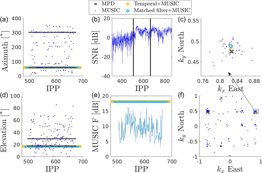
3586 D. Kastinen et al.: Resolving the ambiguous direction of the arrival of weak meteor radar trail echoes
(IPPs). They will also not affect the ambiguity dynamics, as
the gain pattern of all channels are identical.
Ae−ihk,r 1 iR
3
As such, we can assume that the white noise ξ is a complex
8(k) = g(k) .. (1)
.
. circularly symmetric normal distribution for each dimension;
Ae −ihk,r N iR3 i.e. ξ ∼ CN N (0, σ 2 ), which is uncorrelated both in space and
time. The spatial correlation matrix R of our measurements
Here the complex vector 8(k) is the modelled set of com- is calculated as
plex voltages output by the radar system given that the in-
coming wave DOA is k. The r i vectors represent spatial an- R(x) = xx † . (3)
tenna locations and g(k) the combined gain pattern of the
transmitting and receiving antennas. The spatial correlation matrix contains the information of all
possible phase differences between antennas as measured by
3.2 Spatial correlation matrix the radar, as well as the signal power in the diagonal.
We define a measured sensor response as the complex vector 3.3 MUSIC
x ∈ CN . The SKiYMET radar uses a single-pulse transmis-
sion, i.e. no coded transmission sequences, without oversam- A detailed description of the MUSIC implementation we
pling on reception. There is only a single temporal sample of have used is given in Kastinen and Kero (2020). Here, we
the echo for each pulse. Therefore, the sensor response model notate the entire process by a function G that takes as in-
in Eq. (1) directly models a received echo. The measurement put the spatial correlation matrix R and the sensor response
vector x consists of the ideal response 8 ( k ) and additive model 8 ( k ). The function G outputs an estimated DOA k̃
white noise ξ (e.g. Bianchi and Meloni, 2007; Polisensky, and the level at which the sensor response model matched the
2007): measured signal, F :
x = 8(k) + ξ . (2) G(R, 8) = (F, k̃). (4)
However, if the noise is spatially correlated, the cross cor- The quantity F describes the level to which the MUSIC im-
relations between antennas can exhibit noise spikes at zeroth plementation was able to match the used model 8 with the
temporal lag (Holdsworth et al., 2004). Considering the setup measured signal x, which we call the MUSIC response. If
of the system, any spatially correlated noise from galactic there is a perfect match F 7 −→ ∞, while a total mismatch is
sources should be small enough not to impact the main pur- represented by F = 1. We have here adopted the convention
pose of this study, as is discussed further in Appendix A. In- that azimuth measures the angle clockwise from north.
strumental effects (e.g. transmitter and receiver phase noise)
and other users on the same frequency are other potential 3.4 Temporal integration
sources of correlated noise. Other users on the same fre-
quency would essentially be taken care of by the MUSIC al- The key to resolving angular ambiguities is to increase the
gorithm: as the signal subspaces are determined (all of them) SNR of the signals used in the DOA determination by tem-
and the noise subspace is defined as the complement space poral integration. There are many ways to implement tempo-
of only the strongest signal, any such other signal will auto- ral integration. As the local wind speeds at meteor altitudes
matically be filtered away as long as its signal is weaker than are small compared to the distance from the radar, the possi-
the trail echo. Also, the system used in the study is located ble angular change over the typical dynamical lifetime of a
in a rather underpopulated region of northern Finland where meteor trail event is small. This fact allows us to implement
interference in the radio frequency band used does not seem a method based on the assumption that the individual spatial
to be a concern (except the transient ionosonde interference, correlation matrices for each measured radar pulse are prac-
which is easily filtered out; see Sect. 4). tically statistical sample points of the same quantity. Conse-
Another possible effect on the sensor response is mutual quently, this quantity can be temporally integrated to increase
coupling. It is known that mutual coupling introduces phase the SNR of each element of the matrix. The temporally inte-
errors on the signals from individual antennas, resulting in grated spatial correlation matrix is defined as
zenith angle errors of up to 0.5◦ for the Jones configuration
Ns
(Younger and Reid, 2017). We are not applying corrections 1 X
R̄ = R(x(ti )), (5)
specifically for mutual coupling phase errors, but we do ap- Ns i=1
ply the system phase calibration data given in the MPD file.
Regardless, phase errors that are stationary as a function of where there are Ns measured pulses from the trail in ques-
time for a fixed-beam pointing direction and pulse transmis- tion. Equation (5) is essentially the same as the zero lag cross
sion sequence will not decorrelate the temporal integration covariances described in Holdsworth et al. (2004). The the-
of the spatial correlation matrix between inter-pulse periods oretical relation between coherent integrations Ns and SNR
Atmos. Meas. Tech., 14, 3583–3596, 2021 https://doi.org/10.5194/amt-14-3583-2021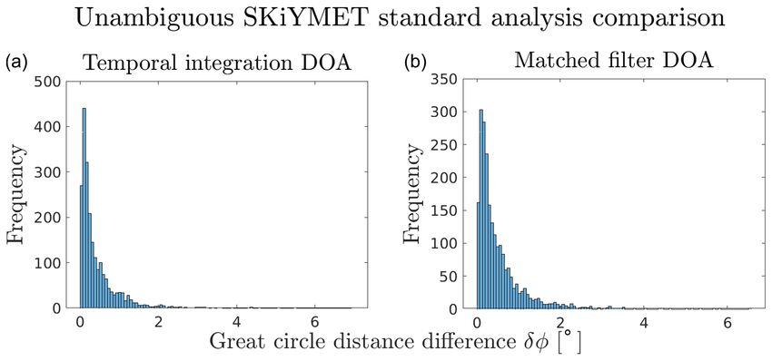
D. Kastinen et al.: Resolving the ambiguous direction of the arrival of weak meteor radar trail echoes 3587
is SNR∝ Ns . Below, we sometimes refer to a set of Ns mea- lar determination. The MUSIC response function is the in-
sured radar pulses as a number of IPPs. Each IPP corresponds verse of a scalar vector projection onto the noise subspace
to ∼ 466 µs of time, i.e. the inverse of the PRF. (Schmidt, 1986). The basis set of the noise subspace will vary
The small angular change allows us to implement a sec- depending on the noise in the signal. The implementation
ond kind of temporal integration given that the radar system we have used of MUSIC sweeps all parameters of a sensor
transmitted phase is predictable. The method assumes that response model to find the sensor response with the small-
the target has drifted less than a radar wavelength between est noise subspace component. This means that even though
subsequent pulses, which is a valid assumption in the case of the noise subspace component of the output point would be
trail echoes. If no other effects that change the phase of the small, the signal space could simply have been displaced to
signal differs between pulses, the drift of the target can be this point by the noise. Thus, the MUSIC response is not a di-
found by the pulse-to-pulse phase difference. More specifi- rect indication of error but simply an indication of how well
cally, applying a filter matched to the phase change on the the sensor response model was able to match the measured
signal allows coherent integration of each channel over the signal subspace. Hence, the mean of the distribution of MU-
entire lifetime of the trail. A matched filter enables more effi- SIC responses increases with SNR but is uncorrelated with
cient coherent integration (further discussed in Appendix A). the true angular error.
We have implemented a matched-filter η(ω), where ω
is the phase velocity. We search for the parameter ωm 3.5 Direct Monte Carlo (DMC)
that maximizes the coherently integrated filter output, i.e.
maxω η(ω) = ωm . This is essentially a simple version of the As outlined in Kastinen and Kero (2020), DMC simulations
coherent deconvolution described in Vierinen et al. (2016). of DOA determinations can resolve the ambiguity dynamics
Specifically, the filter output is of a radar system. Such DMC DOA determination simula-
tions are shown in Fig. 1. Using these simulations, one can
N X Ns 2 match the measured ambiguity pattern with a simulated the-
1 X
η(ω) = xj (tl )eiωtl , (6) oretical one to infer the true DOA of an ambiguous measure-
N j =1 l=1
ment.
where xj (tl ) are signals at time sample tl from channel j . 3.6 Bayesian inference
The optimal matched filter found is then used to coherently
integrate the channel signals as The matching process of comparing a simulated DOA out-
Ns put distribution with a measured one can be done by hand.
X
xm = x(tl )eiωm tl . (7) Ideally, a quantitative and algorithmic approach should be
l=1 used. Kastinen and Kero (2020) showed that a Bayesian ap-
proach is a suitable way to perform systematic and quantita-
Finally, the MUSIC algorithm is applied to the spatial corre- tive matching of simulations to observations. We have imple-
lation matrix of this signal, i.e. on R(x m ). mented a modified version of the method outlined there.
The MUSIC response F is equivalent to SNR for DOA de- Given a model with parameters y which has generated
termination (Schmidt, 1986). Thus, as the MUSIC response observations D, Bayesian inference can be used to find the
F̄ depends on the temporally integrated spatial correlation probability distribution of possible model parameters. This
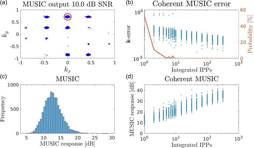
matrix R̄, we expect F̄ ∝ Ns . An example is illustrated in distribution is called the posterior P(y). The posterior is con-
Fig. 1, where ∼ 1 × 10⁴ echoes originating from 0◦ azimuth nected to a prior probability θ (y), i.e. what we think the dis-
and 45◦ elevation were simulated at an SNR of 10 dB for tribution is before any observations. The observed data are
the SKiYMET radar. These echoes were analysed with the used to update the prior distribution by the use of a likeli-
MUSIC algorithm, G. Then, up to 200 of the spatial correla- hood function L. This likelihood function determines how
tion matrices were temporally integrated and used as input to probable the observed data D are, given the model param-
the MUSIC algorithm. The results are illustrated in the right eters y. The relationship between the prior θ , likelihood L,
column of the figure. Here, as expected, sample points tem- and posterior P is given by Bayes’ theorem:
porally integrated at 1 order of magnitude correspond to a
10 dB MUSIC response increase. Additionally, in the upper L(D|y)θ (y)
right panel on the right vertical axis, we illustrate the prob- P(y) = R . (8)
L(D|y 0 )θ (y 0 )dy 0
ability of ambiguous output. In this example, the probability
drops significantly already with 2–3 integrated matrices and Here | indicates conditional probability. In our application,
the ambiguous output DOA behaviour disappears completely the model parameters y are the ambiguous DOA locations
after 10 integrated matrices. labelled by an index y = j .
Even though this shows that SNR and the MUSIC re- The Bayesian approach in Kastinen and Kero (2020)
sponse is perfectly correlated, one must not mistake the MU- used individual DOA measurements and multinomial se-
SIC response for a proxy for absolute precision of the angu- quence generation probabilities to infer the true location.
https://doi.org/10.5194/amt-14-3583-2021 Atmos. Meas. Tech., 14, 3583–3596, 20213588 D. Kastinen et al.: Resolving the ambiguous direction of the arrival of weak meteor radar trail echoes
Figure 1. DMC simulation example showing the effects on DOA determination using MUSIC when temporally integrating the spatial cor-
relation matrix. Approximately 1 × 10⁴ echoes originating from 0◦ azimuth and 45◦ elevation, as marked by the red circle in (a), were
simulated at an SNR of 10 dB for the SKiYMET radar system. These echoes were analysed with the MUSIC algorithm individually; more-
over, up to 200 of the spatial correlation matrices were temporally integrated and analysed. In (a) the MUSIC DOA output for the individual
simulations is illustrated in the wave vector ground projection plane, i.e. kx , ky . In (c) the distribution of MUSIC responses are gathered as a
histogram. Panels (b) and (d) display the results as a function of the number of temporally integrated matrices. The MUSIC response is given
in the panel (d) and the wave vector error in panel (b). Additionally, in the panel (b) on the right vertical axis, we illustrate the probability
of ambiguous output. In this example, the probability drops significantly already with two to three integrated matrices and the ambiguous
output DOA behaviour disappears completely after 10 integrated matrices.
Their approach was designed considering low number statis- generated by a target at the location labelled 2 (given the spe-
tics, i.e. on the order of 10 independent measurements. The cific SNR in the simulation).
SKiYMET system has a high PRF compared to the typical In the current modified Bayesian inference approach we
experimental setups at several of the radar systems that were redefine the likelihood function in terms of simulated and
examined in Kastinen and Kero (2020). Usually, hundreds of measured multinomial parameters. We regard the simulated
received pulses are available from each meteor event. Prac- multinomial parameters as exact and true. The measured
tically, this makes the discrete sequence Bayesian approach multinomial parameters are found by calculating the follow-
unstable if the simulations do not exactly model the proba- ing probabilities:
bility of algorithm failure. Modelling this probability is very
Ns
costly in terms of computational resources. However, as there 1 X 1 if k̃ l ∈ Ai
are generally hundreds of measured sample points one can Pi = P (k̃ ∈ Ai ) ≈ P̃i = , (9)
Ns l=1 0 if k̃ l 6 ∈ Ai
instead calculate the multinomial distribution itself with high
accuracy. The measured multinomial distribution can then be where Ai is the region for an ambiguous DOA. This is iden-
directly compared with the simulated multinomial distribu- tical to computing the expected value of 1 over the measured
tion. A detailed account of how to discretize the DOA distri- sample points or calculating the multinomial maximum like-
bution into a multinomial distribution was given in Kastinen lihood estimator. Given enough sample points, the central
and Kero (2020). The description includes information both limit theorem applies and the multinomial probability esti-
on how multinomial probabilities are generated from the di- mator can be regarded as normal. It is therefore equivalent
rect Monte Carlo (DMC) simulations, here denoted P̂ij , and to the Bernoulli mean estimator distribution. The estimator
probabilities calculated from measurements, denoted P̃i . The variance can be approximated by substituting the distribution
index i denotes a possible, ambiguous DOA location, while variance with the measured Bernoulli variance (Papoulis and
the index j denotes the true location. As an example, the no- Pillai, 2002):
tation P̂12 = 0.25 would mean that there is a 25 % probability
that ambiguity location 1 is the output from a measurement
Atmos. Meas. Tech., 14, 3583–3596, 2021 https://doi.org/10.5194/amt-14-3583-2021D. Kastinen et al.: Resolving the ambiguous direction of the arrival of weak meteor radar trail echoes 3589
matrix of matched-filter integrated channel signals (R(x m )),
and Bayesian inference based on DMC simulations of DOA
P̃i (1 − P̃i ) determinations (P(j )). We have compared all four methods
var(P̃i ) ≈ . (10)
Ns in order to test and validate them.
In total 2222 events were automatically analysed. To select
For the special case of P̃i = 0 (corresponding to no measure- authentic specular trail echoes we used the time for which
ments in an inclusion region Ai ) we have implemented an the amplitude of the backscattered signal falls to one half of
estimator variance similar to the considerations in Hanley its maximum value τ . We did not include events with unde-
and Lippman-Hand (1983) and defined var(P̃i ) = − ln(0.05) 2Ns . termined τ (these may be ground echoes or long-lived non-
Then, the modified likelihood function can be written in log specular echoes (Kozlovsky et al., 2019, 2020; Bronshten,
form as 1983, pp. 356)), τ less than 0.001 s (these may be ionosonde
XNo q
1 (P̂ij − P̃i )2 interference), or radial velocities exceeding 100 m/s (these
ln(L(j )) = − ln var(P̃i )2π − , (11) may be due to Farley–Buneman instabilities (Kelley, 2009))
2 var(P̃i )
i=1 as such events are unlikely to be genuine specular trail
echoes. Some of the events still appear likely to have been
where No is the number of ambiguous regions.
range-spread non-specular trail echoes (e.g. the “straight
To avoid contamination of the probabilities by faulty IPP
line” of black dots in Fig. 5 around kx = −0.15, ky = 0.25
selection, i.e. selecting IPPs that do not contain a valid echo
all occurred within 1.5 s of each other), but as this does not
from the trail, we only use the ambiguous locations as pa-
impact the DOA evaluation, we did not attempt to remove
rameters in the multinomial distribution and do not include
such events from the analysis. By contrast, the methods pre-
an algorithm failure probability.
sented here can be used to successfully analyse such events.
As we have no prior information on the location of the
A summary of the analysis results is given in Table 1.
target, Bayes’ theorem from Eq. (8) reduces to
Out of the total of 2222 events 294 were listed as hav-
L(j ) ing angular ambiguities. These were analysed with both the
P(j ) = P . (12) DMC-simulation-based Bayesian inference and the tempo-
L(j )
j ral integration versions of MUSIC. An example of such an
event is illustrated in Fig. 2. The upper middle panel illus-
3.7 Automation trates SNR versus radar pulse, and the two vertical black lines
denote the region within which the trail event was identified
To facilitate testing on a wide range of events we have created
by the SKiYMET analysis. These are the pulses that were
an automated routine to read in an MPD file, iterate through
also reanalysed using the MUSIC algorithm. The DOA out-
each event, and reanalyse the events using the CEV files. For
put from these IPPs is illustrated as blue dots in the left and
each event we apply MUSIC to each pulse individually, as
right column of panels. The upper left panel shows azimuth
well as on the temporally integrated spatial correlation ma-
as a function of IPP and the lower one elevation. Here, the
trix, and perform a matched-filter search that maximizes the
transparent grey lines denote the azimuth and elevation given
coherently integrated filter output, i.e. maxω η(ω) = ωm . Us-
in the MPD file. In this case, the standard SKiYMET analy-
ing the phase velocity found, ωm , we apply phase correction
sis produced two angular ambiguities. The orange transpar-
to each individual channel and calculate MUSIC using the
ent line denotes the DOA output from the R̄-based MUSIC
resulting spatial correlation matrix.
and the cyan transparent line denotes the DOA output from
If the event was flagged with angular ambiguities in the
the R(x m )-based MUSIC. The same information is given in
MPD file, an ambiguity search is run and a series of DMC
wave vector ground-projected space, kx , ky in the lower right
DOA determination simulations, again using MUSIC, are
panel with a zoomed-in version in the upper right panel. Here
executed. Using these DMC simulations and the ambiguity
the MPD-file results are marked by grey crosses, the R̄-based
analysis we discretize the measurements and the DMC simu-
MUSIC by an orange circle, the R(x m )-based MUSIC by a
lations into input and output locations. The probability distri-
cyan circle, and the regular MUSIC output for each IPP is
bution over these locations is used in the Bayesian inference
marked by the blue dots. Finally, the distribution of the MU-
to calculate an input DOA probability. All the results, simu-
SIC response F is illustrated in the lower middle panel as
lations and auxiliary data are then cached to disk. These data
a function of IPP. Here, the solid lines denotes the MUSIC
are available in the associated open-data repository.
response for the temporally integrated versions.
For each of the 294 events with angular ambiguities we
4 Results also performed a series of DMC DOA determination simula-
tions. The noise in the simulations was set to sample from the
We have four independent methods of determining the DOA: distribution of SNRs measured for the events themselves so
the SKiYMET standard data product, temporal integration as to reproduce the multinomial probabilities. In Fig. 3, the
of the spatial correlation matrix (R̄), the spatial correlation simulations and the Bayesian inference results are illustrated
https://doi.org/10.5194/amt-14-3583-2021 Atmos. Meas. Tech., 14, 3583–3596, 20213590 D. Kastinen et al.: Resolving the ambiguous direction of the arrival of weak meteor radar trail echoes
Table 1. Summary of the analysis results.
Total events analysed 2222
DOA unambiguous 87 % (1928 of 2222)
Matched filter, temporal integration and MPD concur 100 % (1928 of 1928)
DOA ambiguous 13 % (294 of 2222)
Matched filter resolved 100 % (294 of 294)
Temporal integration resolved 100 % (294 of 294)
Matched filter and temporal integration concur 98 % (289 of 294)
New temporal integrated solution 1 % (4 of 294)
New matched-filter solution 1 % (4 of 294)
DMC simulations 294
Anomalous signal 13 % (38 of 294)
Nominal signal 87 % (256 of 294)
Matched filter concur 96 % (245 of 256)
Temporal integration concur 96 % (246 of 256)
All concur 95 % (243 of 256)
New Bayes solution 3 % (7 of 256)
Figure 2. Meteor recorded on 13 December 2018 00:03:27.302 UTC. Panel (b) illustrates SNR versus IPP and the two vertical black lines
denotes when the event occurred. This particular example was randomly picked from a list of ambiguous events. It is likely an overdense
echo, but this does not affect the DOA determination. This event had three range ambiguities (187.9, 257.9, and 327.9 km) and two angular
ambiguities. The peak SNR was 8.7 dB. The two angular ambiguities are marked by grey horizontal lines in (a) (azimuth) and (d) (elevation).
The MUSIC DOA output from individual IPPs are illustrated as blue dots, while the light blue and orange transparent lines denote the
DOA output after temporal integration with and without matched-filter optimization, respectively. The lines are of different widths only to
enhance visibility. The same information is given in wave vector ground-projected space, kx , ky , in (c, f). Finally, the distribution of MUSIC
responses F as a function of IPP is illustrated in (e). Here, the horizontal lines denote the MUSIC response for the temporally integrated
spatial correlation matrices.
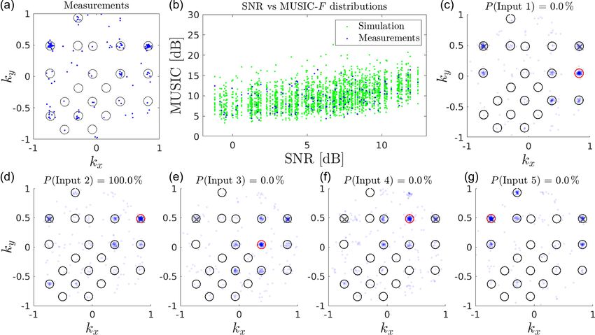
alongside the measurement data for the event, also illustrated middle panel shows the measured distribution of the SNR
in Fig. 2. The upper left panel shows the MUSIC DOA out- versus MUSIC response compared to the simulated distri-
put in wave vector ground-projected space, i.e. kx and ky . bution. The remaining panels show DMC DOA determina-
The black circles denote the possible ambiguities and their tion simulations with different true inputs. In each of these
inclusion regions, i.e. the Ai sets from Eq. (9). The upper panels, the input DOA is marked by the large red circle. For
Atmos. Meas. Tech., 14, 3583–3596, 2021 https://doi.org/10.5194/amt-14-3583-2021D. Kastinen et al.: Resolving the ambiguous direction of the arrival of weak meteor radar trail echoes 3591
reference, the MPD-file results are also marked by transpar- could confirm this interpretation. If multiple coherent
ent grey crosses in each panel. The title of these figures give signals are present, there is more than one large MUSIC
the Bayesian inference results P(j ) in percent rounded to eigenvalue (Schmidt, 1986).
one decimal. The Bayesian inference can also be evaluated
– For the remaining events that did not concur, upon man-
manually by comparing the simulated distribution of DOA
ual inspection no events could be identified in these
outputs with the measurements given in the upper left panel.
cases and the signal appeared to be only background
In this case, the Bayesian inference and the temporally inte-
noise. Hence they were not examined further.
grated MUSIC, as well as a manual inspection, all agree and
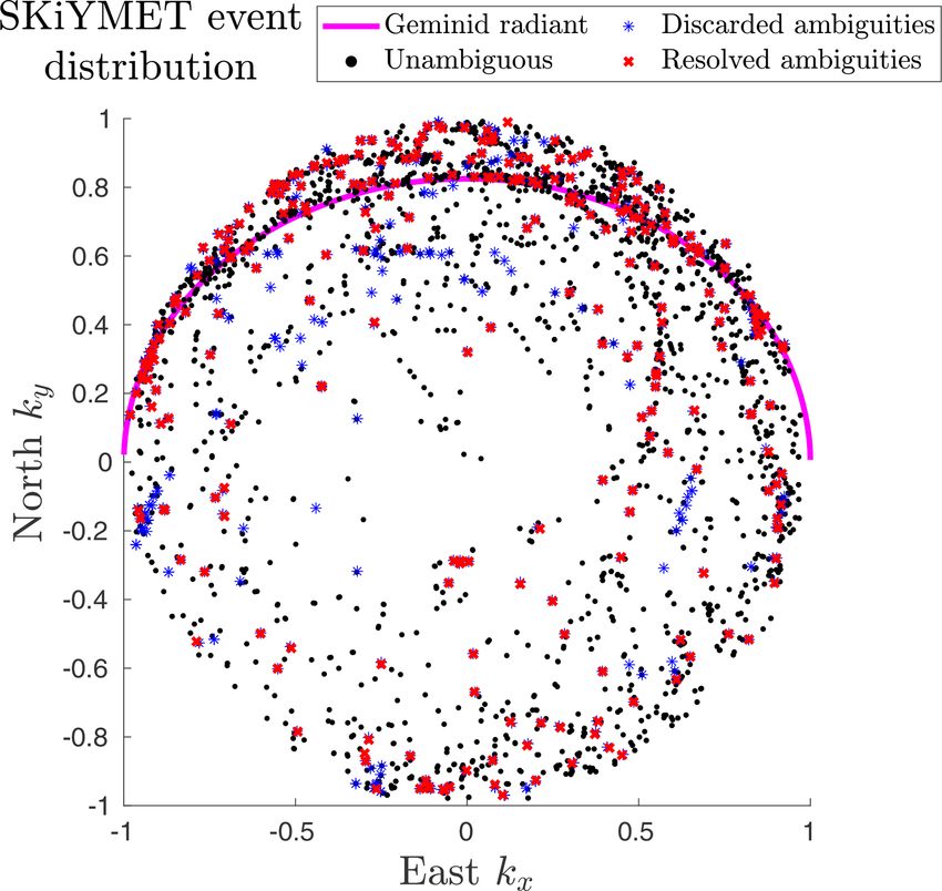
identify the same DOA as the true location. The DOA distribution for all analysed events is illustrated
Of the 294 analysed events, 256 (87 %) were identified in Fig. 5. The black dots are the 1928 unambiguous meteor
as containing a nominal echo, ideally scattered from a sin- trail events, the blue stars are the original ambiguous nominal
gle meteor trail. The remaining 38 events (13 %) contained signal locations that could be discarded, and the red crosses
anomalous signals in the sense that the target model does not are the 249 resolved ambiguities for which the Bayes solu-
match with the real target(s). The SNR of individual pulses tion matched with one of the listed ambiguous locations in
in each event typically span several orders of magnitude. The the original SKiYMET analysis. There are multiple blue stars
mismatch of model and reality was detected automatically by per resolved ambiguous event, i.e. per red cross.
using the fact that the MUSIC F value did not increase with The DOA distribution is concentrated towards low ele-
increasing SNR as a criterion. This indicates that regardless vation in the north. These data were recorded during the
of the measured signal strength, the sensor response model Geminid meteor shower. The solid line shows the locations
could not be matched to the detected signal. Further exami- where specular reflection could occur assuming that the me-
nation to identify the sources or causes of these anomalous teor originated from the centre of the Geminid meteor shower
events was considered outside the scope of this study. The radiant region (right ascension 112◦ , declination 33◦ ) at the
events were marked as anomalous signals in Table 1 and were time of the measurement.
not processed further. At around 00:00 UTC, the Geminid radiant as well as most
In 95 % of the nominal ambiguous echoes, all three non- sporadic meteor source regions were located towards the
SKiYMET methods found one and the same output DOA, south (Wiegert et al., 2009) since Sodankylä is located at a
and this DOA was listed as one of the possible ambiguous high northern latitude. Therefore, most meteors with trajec-
DOAs in the original SKiYMET analysis. Similarly, in all tories fulfilling a specular condition with respect to the radar
unambiguous cases with a nominal signal, the results from all appeared towards the north. This explains the concentration
three methods also concurred. For the unambiguous cases a of DOAs towards the north at low elevation in Fig. 5.
comparison between the temporally integrated MUSIC algo- When the remaining resolved direction only has one am-
rithms and the SKiYMET standard data product is illustrated biguous range possibility within the meteor zone, the re-
in Fig. 4. This further validates the robustness of the im- solved angular ambiguity also solves the range ambiguity
plementation as their difference is typically less (root mean problem, but this is not always the case. The problem with
square differences are 0.68◦ for the temporal integration re- range ambiguities is independent from the angular ambigu-
sults and 0.79◦ for the matched-filter results) than the re- ity problem and outside of the scope of this study. How-
ported expected angular measurement accuracy of the system ever, the range ambiguity would be easily avoided with an
(≈ 1◦ , Jones et al., 1998). update of the system to use coded transmission sequences.
Upon manual examination of the remaining 5 % where all An advanced example is give by Vierinen et al. (2016), who
three methods did not find one and the same DOA, the fol- used coded transmission sequences with a multiple-input–
lowing observations were made: multiple-output bi-static and continuous-wave setup. In the
case of the mono-static Sodankylä SKiYMET system, it
– In five of the cases where the Bayesian inference indi-
would be enough to use a small set of binary-phase shift
cated a solution not listed in the MPD file, the event had
key codes on the pulsed transmitter to enable distinguishing
too few IPPs to be well determined by any method. In
between the pulse trains that come from subsequent echoes
the other two events, both the R̄ and the R(x m ) solu-
within the meteor zone.
tions concurred with P(j ) and manual inspection indi-
The reason why range ambiguities appear in the stan-
cated they were correct.
dardized SKiYMET analysis is the combination of uncoded
– There were a few cases where the R(x m ) yielded a good radar pulses and high PRF. At low-elevation angles from the
match while R̄ decorrelated. We attribute this to simul- radar, this means that two or more consecutively transmit-
taneous targets in the same range gate but with different ted pulses may simultaneously give rise to echoes of mete-
drift speeds. This would explain why the matched filter ors in the standardized acceptable altitude range 70–110 km
was able to yield a good match (optimization towards a (Hocking et al., 2001). The commonly used PRF 2144 Hz of
single target) while R̄ would not. A thorough MUSIC the SKiYMET radar systems corresponds to a range aliasing
eigenvalue and matched-filter local maximum analysis of ' 70 km.
https://doi.org/10.5194/amt-14-3583-2021 Atmos. Meas. Tech., 14, 3583–3596, 20213592 D. Kastinen et al.: Resolving the ambiguous direction of the arrival of weak meteor radar trail echoes
Figure 3. Summary of the DOA determination simulations and the Bayesian inference results for the meteor in Fig. 2. Five different possible
true DOAs were identified and their individual DMC simulations are illustrated in (c–g). The Bayesian probability of an input DOA being the
true location of the trail is given in the title. In each of these panels, the input DOA is marked by a large red circle and the MPD-file results
are marked by grey crosses. The measured DOA output distribution is given in (a). The black circles denote the possible ambiguities and
their inclusion regions. The temporal integration and matched-filter results illustrated in Fig. 2 coincide with the largest probability location
here. Panel (b) shows the measured and simulated distributions of MUSIC response F versus SNR.
Figure 4. Comparison between the nominal signal SKiYMET standard data products and the temporal integration R̄-based MUSIC DOA
solutions (a) as well as the matched-filter R(x m )-based MUSIC DOA solutions (b). The difference between the solutions is measured as
great-circle angular distance between the DOAs. In total 1928 unambiguous trail events were included in the histograms. The root mean
square differences are 0.68◦ for the temporal integration results and 0.79◦ for the matched-filter results.
5 Conclusions Bayesian inference, many simultaneous DMC simulations
are required, and this method is as such computationally ex-
pensive. However, as the results can be used to validate other
We have shown that DMC simulations can characterize the methods and characterize the behaviour of a radar system,
DOA determination behaviour of a system and validate the they are a valuable tool for development work.
performance of other analysis methods. Together with a We have implemented two versions of standard tem-
Bayesian inference approach, these simulations can system- poral integration techniques used to increase the SNR of
atically be used to determine the true location of weak me- the spatial correlation matrix and subsequent application of
teor radar trail echoes with ambiguous DOA. To perform the
Atmos. Meas. Tech., 14, 3583–3596, 2021 https://doi.org/10.5194/amt-14-3583-2021D. Kastinen et al.: Resolving the ambiguous direction of the arrival of weak meteor radar trail echoes 3593
Standard meteor trail radar systems, such as SKiYMET
(Hocking et al., 2001) generally produce enough sample
points from each registered meteor for the temporally inte-
grated MUSIC to work. The results indicate that this method
will solve the angular ambiguity problem in almost all cases.
The problem with range ambiguities is independent from
the angular ambiguity problem and outside the scope of this
study, but we note that it could be avoided with an update of
the system to use coded transmission sequences.
The presented methods do not depend on the MUSIC al-
gorithm per se: for example, the complex signal amplitudes
that are used in the DOA determination algorithm by Jones
et al. (1998) to calculate the φ angles can be temporally in-
tegrated in the same way as the spatial correlation matrix R
was temporally integrated here.
Finally, one can pose the question whether and at what
point the temporally integrated MUSIC becomes ambiguous.
This question as well as the validation of a pipeline imple-
menting temporal integration techniques can be addressed by
the same type of DMC simulations.
Figure 5. Illustration of the DOA distribution of 2222 events in
Sodankylä SKiYMET meteor radar data before and after applying
temporal integration. The black dots are the unambiguous meteor
trail events, the blue stars are the original ambiguous locations that
could be discarded, and the red crosses are the resolved ambiguities
after temporal integration. There are multiple blue stars per event
and red cross. The data were recorded during the Geminid meteor
shower. The solid line illustrates directions that fulfil the specular
condition for meteors arriving from the Geminid radiant.
the MUSIC algorithm. This is computationally inexpensive
and implementation-wise a very simple method able to re-
solve ambiguous DOAs for SKiYMET meteor radar sys-
tems. However, even though the concept itself is not new (cf.
Holdsworth, 2005; Vierinen et al., 2016), it does not seem
to have been implemented in the SKiYMET standard data
analysis. Both the temporally integrated spatial correlation
matrix version of MUSIC and the matched-filter version pro-
vided the correct output DOA according to the Bayesian in-
ference in ∼ 96 % of the ambiguous cases containing a nom-
inal signal. In the cases when they did not agree, there were
either not enough sample points to temporally integrate for
the method to be effective or we could not manually con-
form a specular meteor trail echo in the raw data. For all un-
ambiguous cases both methods coincide with the SKiYMET
standard data product.
https://doi.org/10.5194/amt-14-3583-2021 Atmos. Meas. Tech., 14, 3583–3596, 20213594 D. Kastinen et al.: Resolving the ambiguous direction of the arrival of weak meteor radar trail echoes
Appendix A: Temporal integration of cross correlations The expected noise power is given by the noisy signal vari-
ance when A = 0, i.e. PNoise = Nt σ 4 . Therefore, the “SNR”
Extending the definition used in Eqs. (1) and (2) to include for a cross-correlated signal would be defined as
temporal variations we define
" # 2
Nt
−i(hk n ,r j iR3 −φn )
8̃j,n 8̃∗l,n
P
8j,n = gj (k n )An e , (A1) E 4
n=1 Nt2 A4 A
8̃j,n = 8j,n + ξj,n , (A2) = = N t . (A7)
Nt σ 4 Nt σ 4 σ
where n denotes the temporal component and the noise is
There is no standardized definition of coherent integra-
ξj,n ∼ CN (0, σn2 ), i.e. a complex circularly symmetric nor-
tion other than that such an integration should integrate
mal random variable. Here k n is the incident wave vector,
the quadrature components of the signal envelope by taking
An is the wave amplitude, h, iR3 is the inner product, r j is the
phase into account (e.g. Miller and Bernstein, 1957). As the
physical location of antenna j , and gj is its gain pattern. We
phases of the cross correlation signal are preserved by the
will assume that the noise is uncorrelated between samples
temporal integration of cross correlations, it is essentially the
of j and between samples of n. In reality, if there is a par-
cross correlation envelope that is integrated; i.e., as the com-
ticularly strong point source of noise compared to the overall
ponent e−i(hk,r j −r l iR3 does not change, a simple summation
background noise, the total noise picked up by an antenna
can be referred to as coherent integration. However, a more
may become spatially correlated. There are galactic sources
efficient coherent integration would be to apply a matched-
that produce such noise (Gaensler, 2004). However, given the
filter integration prior to cross correlation.
low directivities of the SKiYMET antennas and the fact that
Assuming a matched filter has perfectly modelled the tem-
it is a single-pulse system, assuming completely uncorrelated
poral component of the signal φn , the statistical moments of
noise is acceptable for this derivation.
the cross correlation of the matched-filter integration would
For simplicity, we will make the following further assump-
be
tions for Eq. (A2): individual antenna gain is unity gj = 1;
signal amplitude is constant over antennas and time An = A; "
XNt
!
Nt
X
!#
−iφn ∗ iφm
the wave vector change due to the local wind drift velocity E 8̃j,n e 8̃l,m e =
over the meteor trail event time is negligible k n = k. The ex- n=1 m=1
pected value and variance of the signal is Nt X
X Nt h i
h i = E (Ae−ihk,r j iR3 + ξj,n )(Aeihk,r l iR3 + ξl,m ) =
E 8̃j,n = 8j,n , (A3) n=1 m=1
h i Nt X
X Nt
Var 8̃j,n = σ 2 . (A4) = A2 e−ihk,r j −r l iR3 =
n=1 m=1
When stochastic variables are uncorrelated, the ex- = Nt2 A2 e−ihk,r j −r l iR3 , (A8)
pected value operator is linear and multiplicative, i.e. "
Nt
!
Nt
!#
X X
E[XY ] = E[X]E[Y ], while the variance operator is linear Var 8̃j,n e −iφn ∗
8̃l,m e iφm
=
and follows Var[XY ] = |E[X]|2 Var[Y ] + |E[Y ]|2 Var[X] + n=1 m=1
Var[X]Var[Y ]. This applies also to complex random vari- Nt X
X Nt h i
ables (O’Donoughue and Moura, 2012). As such, the mo- = Var (Ae−ihk,r j iR3 + ξj,n )(Aeihk,r l iR3 + ξl,m ) =
ments of a spatial cross correlation of Eq. (A2) integrated n=1 m=1
over time are Nt X
X Nt
"
Nt
#
Nt
= 2A2 σ 2 + σ 4 = Nt2 (2A2 σ 2 + σ 4 ).
h i h i
n=1 m=1
X X
∗
E 8̃j,n 8̃l,n = E 8̃j,n E 8̃∗l,n =
n=1 n=1 Here we have used the fact that complex rotations of ξ do
= Nt A2 e−i(hk,r j −r l iR3 , (A5) not affect the distribution as it is circularly symmetrical. This
shows that a perfect matched-filter integration prior to cross
" # correlation would produce a more effective coherent integra-
Nt Nt
X X h i tion. The SNR for the latter cross-correlated signal is
Var 8̃j,n 8̃∗l,n = Var 8̃j,n 8̃∗l,n =
n=1 n=1 4
Nt4 A4 2 A
Nt i2 i2 = Nt . (A9)
Nt2 σ 4
h h i h h i
σ
X
= E 8̃j,n Var 8̃∗l,n + E 8̃∗l,n Var 8̃j,n
n=1
h i h i
+ Var 8̃j,n Var 8̃∗l,n = Nt (2A2 σ 2 + σ 4 ). (A6)
Atmos. Meas. Tech., 14, 3583–3596, 2021 https://doi.org/10.5194/amt-14-3583-2021D. Kastinen et al.: Resolving the ambiguous direction of the arrival of weak meteor radar trail echoes 3595
Data availability. The data described in Sect. 2.2 that were anal- Hocking, W. K., Fuller, B., and Vandepeer, B.: Real-time de-
ysed, i.e. the confirmed event (CEV) files and the meteor position termination of meteor-related parameters utilizing modern
data (MPD) file, are available at https://doi.org/10.5878/vnhd-na43 digital technology, J. Atmos. Sol.-Terr. Phy., 63, 155–169,
(Kastinen et al., 2020) together with a short description of their https://doi.org/10.1016/S1364-6826(00)00138-3, 2001.
structure. Holdsworth, D. A.: Angle of arrival estimation for all-sky in-
terferometric meteor radar systems, Radio Sci., 40, RS6010,
https://doi.org/10.1029/2005RS003245, 2005.
Author contributions. DK developed the analysis and model code Holdsworth, D. A., Reid, I. M., and Cervera, M. A.: Buckland Park
and performed the simulations and data analysis. AK and ML pro- all-sky interferometric meteor radar, Radio Sci., 39, RS5009,
vided the data set analysed. DK prepared the paper with contribu- https://doi.org/10.1029/2003RS003014, 2004.
tions from JK and AK. All the authors contributed to proofreading Jones, J., Webster, A. R., and Hocking, W. K.: An improved interfer-
the paper. ometer design for use with meteor radars, Radio Sci., 33, 55–65,
https://doi.org/10.1029/97RS03050, 1998.
Kastinen, D. and Kero, J.: A Monte Carlo-type simulation
Competing interests. The authors declare that they have no conflict toolbox for Solar System small body dynamics: Application
of interest. to the October Draconids, Planet. Space Sci., 143, 53–66,
https://doi.org/10.1016/j.pss.2017.03.007, 2017.
Kastinen, D. and Kero, J.: Probabilistic analysis of ambigui-
ties in radar echo direction of arrival from meteors, Atmos.
Acknowledgements. The authors would like to thank David
Meas. Tech., 13, 6813–6835, https://doi.org/10.5194/amt-13-
Holdsworth and Joel Younger for valuable comments and sugges-
6813-2020, 2020.
tions that improved the first version of the paper.
Kastinen, D., Kozlovsky, A., Lester, M., and Kero, J.: Re-
solving ambiguous direction of arrival of weak meteor
radar trail echoes, Swedish Institute of Space Physics,
Review statement. This paper was edited by Jorge Luis Chau and https://doi.org/10.5878/vnhd-na43, 2020.
reviewed by Joel Younger and David Holdsworth. Kelley, M. C.: The Earth’s ionosphere: plasma physics and electro-
dynamics, Academic Press, Cambridge, Massachusetts, United
States, https://doi.org/10.1016/B978-0-12-404013-7.X5001-1,
2009.
Kero, J., Campbell-Brown, M. D., Stober, G., Chau, J. L., Math-
References ews, J. D., and Pellinen-Wannberg, A.: Radar Observations
of Meteors, in: Meteoroids: Sources of Meteors on Earth and
Bianchi, C. and Meloni, A.: Natural and man-made terrestrial elec- Beyond, edited by: Ryabova, G. O. and, Asher, D. J., and
tromagnetic noise: an outlook, Ann. Geophys.-Italy, 50, 435– Campbell-Brown, M. J., Cambridge University Press, 65–89,
445, 2007. https://doi.org/10.1017/9781108606462, 2019.
Bronshten, V. A.: Physics of Meteoric Phenomena, Kluwer, Dor- Kozlovsky, A., Shalimov, S., Oyama, S., Hosokawa, K., Lester, M.,
drecht, The Netherlands, 1983. Ogawa, Y., and Hall, C.: Ground Echoes Observed by the Me-
Brown, P., Spalding, R. E., ReVelle, D. O., Tagliaferri, teor Radar and High-Speed Auroral Observations in the Sub-
E., and Worden, S. P.: The flux of small near-Earth storm Growth Phase, J. Geophys. Res.-Space, 124, 9278–9292,
objects colliding with the Earth, Nature, 420, 294–296, https://doi.org/10.1029/2019JA026829, 2019.
https://doi.org/10.1038/nature01238, 2002. Kozlovsky, A., Lukianova, R., and Lester, M.: Occurrence and Al-
Ceplecha, Z., Borovička, J., Elford, W. G., Revelle, D. O., titude of the Long-Lived Nonspecular Meteor Trails During Me-
Hawkes, R. L., Porubčan, V., and Šimek, M.: Meteor teor Showers at High Latitudes, J. Geophys. Res.-Space, 125,
Phenomena and Bodies, Space Sci. Rev., 84, 327–471, e27746, https://doi.org/10.1029/2019JA027746, 2020.
https://doi.org/10.1023/A:1005069928850, 1998. Lovell, A. C. B., Prentice, J. P. M., Porter, J. G., Pearse, R. W. B.,
Chau, J. L. and Clahsen, M.: Empirical Phase Calibration for Multi- and Herlofson, N.: Meteors, comets and meteoric ionization,
static Specular Meteor Radars Using a Beamforming Approach, Rep. Prog. Phys., 11, 389–454, https://doi.org/10.1088/0034-
Radio Sci., 54, 60–71, https://doi.org/10.1029/2018RS006741, 4885/11/1/313, 1947.
2019. McKinley, D. W. R.: Meteor Science and Engineering, McGraw-
Gaensler, B. M.: Radio Emission from the Milky Way, in: Milky Hill Series in Engineering Sciences, McGraw-Hill Book Com-
Way Surveys: The Structure and Evolution of our Galaxy, edited pany, Inc., USA, 309 pp., 1961.
by: Clemens, D., Shah, R., and Brainerd, T., Astronomical So- Miller, K. and Bernstein, R.: An analysis of coherent integration
ciety of the Pacific (ASP), ASP Conference Series, Utah Valley and its application to signal detection, IRE T. Inform. Theor., 3,
University, 217, 2004. 237–248, https://doi.org/10.1109/TIT.1957.1057425, 1957.
Hanley, J. A. and Lippman-Hand, A.: If nothing goes wrong, is O’Donoughue, N. and Moura, J. M. F.: On the Product of Inde-
everything all right?: interpreting zero numerators, Jama, 249, pendent Complex Gaussians, IEEE T. Signal Proces., 60, 1050–
1743–1745, 1983. 1063, 2012.
Hocking, W. K.: A new approach to momentum flux determinations Papoulis, A. and Pillai, S. U.: Probability, random variables, and
using SKiYMET meteor radars, Ann. Geophys., 23, 2433–2439, stochastic processes, Tata McGraw-Hill Education, McGraw Hill
https://doi.org/10.5194/angeo-23-2433-2005, 2005.
https://doi.org/10.5194/amt-14-3583-2021 Atmos. Meas. Tech., 14, 3583–3596, 2021You can also read