Improved constraints on reionisation from CMB observations: A parameterisation of the kSZ effect
←
→
Page content transcription
If your browser does not render page correctly, please read the page content below
Astronomy & Astrophysics manuscript no. main                                                                                        c ESO 2020
                                               June 19, 2020

                                                    Improved constraints on reionisation from CMB observations:
                                                               A parameterisation of the kSZ effect
                                                                              A. Gorce1, 2 , S. Ilić3, 4, 5 , M. Douspis1 , D. Aubert6 , and M. Langer1

                                                     1
                                                         Université Paris-Saclay, CNRS, Institut d’Astrophysique Spatiale, 91405, Orsay, France
                                                         e-mail: adelie.gorce@ias.u-psud.fr
                                                     2
                                                         Department of Physics, Blackett Laboratory, Imperial College, London SW7 2AZ, U.K.
                                                     3
                                                         CEICO, Institute of Physics of the Czech Academy of Sciences, Na Slovance 2, Praha 8, Czech Republic
                                                     4
                                                         Université PSL, Observatoire de Paris, Sorbonne Université, CNRS, LERMA, F-75014, Paris, France
                                                     5
                                                         IRAP, Université de Toulouse, CNRS, CNES, UPS, Toulouse, France
arXiv:2004.06616v2 [astro-ph.CO] 18 Jun 2020

                                                     6
                                                         Observatoire Astronomique de Strasbourg, Université de Strasbourg, CNRS UMR 7550, 11 rue de l’Université, 67000 Strasbourg,
                                                         France
                                                    Received *********; accepted *******

                                                                                                                 ABSTRACT

                                                    We show that, in the context of patchy reionisation, an accurate description of the angular power spectrum of the kinetic Sunyaev-
                                                    Zel’dovich (kSZ) effect is not possible with simple scaling relations between the amplitude of the spectrum and global parameters,
                                                    such as the reionisation midpoint and its duration. We introduce a new parameterisation of this spectrum, based on a novel description
                                                    of the power spectrum of the free electrons density contrast Pee (k, z) in terms of the reionisation global history and morphology. We
                                                    directly relate features of the spectrum to the typical ionised bubble size at different stages in the process and, subsequently, to the
                                                    angular scale at which the patchy kSZ power spectrum reaches its maximum. We successfully calibrated our results on a custom set of
                                                    advanced radiative hydrodynamical simulations and later found our parameterisation to be a valid description of a wide range of other
                                                    simulations and, therefore, reionisation physics. In the end, and as long as the global reionisation history is known, two parameters
                                                    are sufficient to derive the angular power spectrum. Such an innovative framework applied to cosmic microwave background data and
                                                    combined with 21cm intensity mapping will allow a first consistent detection of the amplitude and shape of the patchy kSZ signal,
                                                    giving in turn access to the physics of early light sources.
                                                    Key words. Cosmology: dark ages, reionization, first stars – cosmic background radiation – Methods: analytical

                                               1. Introduction                                                           (Lewis et al. 2000, Howlett et al. 2012)1 , the reionisation sce-
                                                                                                                         nario used is a step-like transition of xe (z), where the global
                                                   From the launch of the Cosmic Background Explorer                     ionised fraction jumps from 10% to 75% over a (fixed) redshift
                                               (COBE) in 1989 to the publication of the latest results of the            interval of ∆z = 1.73 (Planck Collaboration et al. 2016a). How-
                                               Planck satellite in 2018 (Planck Collaboration et al. 2018), the          ever, this parameterisation does not match simulations and ob-
                                               study of the cosmic microwave background (CMB) has trig-                  servations well since we expect the ionisation fraction to slowly
                                               gered a tremendous amount of research. Cosmological parame-               rise when the first sources light up, before taking off as soon as
                                               ters have been estimated with exquisite precision and our knowl-          about 20% of the IGM is ionised (Robertson et al. 2015, Greig &
                                               edge of cosmic inflation has been greatly improved. Along the             Mesinger 2016, Gorce et al. 2018). This minimal model can have
                                               line of sight, the primordial part of the CMB signal is largely           a huge impact on reionisation constraints: The value of τ inferred
                                               modified by the interaction of CMB photons with structures that           from Planck 2016 data varies from 0.066 ± 0.016 for a step-like
                                               formed later in the Universe. Notably, their interaction with free        process to 0.058 ± 0.012 for a more accurate description (Dous-
                                               electrons in the intergalactic medium (IGM) modify the shape              pis et al. 2015; Planck Collaboration et al. 2016b). It is therefore
                                               and amplitude of the measured CMB temperature and polarisa-               essential to take the asymmetric evolution of xe (z) into account
                                               tion power spectra. The presence of these electrons is the result,        when trying to accurately constrain reionisation, and global pa-
                                               in particular, of cosmic reionisation, an era potentially extending       rameters such as the reionisation midpoint zre and duration ∆z
                                               from a redshift of z ∼ 15 to z ∼ 5 when the first galaxies are            are not sufficient.
                                               thought to have ionised the neutral hydrogen and helium in the                CMB photons can also gain energy from scattering off elec-
                                               surrounding IGM.                                                          trons with a non-zero bulk velocity relative to the CMB rest-
                                                   CMB photons lose energy from scattering off low-energy                frame in a process called the kinetic Sunyaev-Zel’dovich effect
                                               electrons. In CMB data analysis, this effect is accounted for             (hereafter kSZ effect, see Zeldovich & Sunyaev 1969; Sunyaev
                                               when computing the Thomson optical depth. To do so, one needs             & Zeldovich 1980). This interaction adds power to the CMB
                                               to assume a global history of reionisation, that is, a redshift-          temperature spectrum on small angular scales (` & 2000, that is
                                               evolution for the IGM global ionised fraction xe (z). In stan-            smaller than about 5 arcminutes), where secondary anisotropies,
                                               dard Boltzmann solvers which are used to compute theoreti-
                                                                                                                          1
                                               cal predictions in CMB data analysis such as the CAMB code                     Available at https://camb.info.

                                                                                                                                                                    Article number, page 1 of 14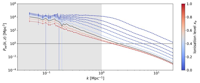
A&A proofs: manuscript no. main

including kSZ, dominate the signal. The impact of kSZ on the           at ` = 3000. For their own work, Shaw et al. (2012) there-
CMB power spectrum is often split between the homogeneous              fore choose a completely different approach: they use hydrody-
kSZ signal, which come from the Doppler shifting of photons            namical simulations to map the gas density to the dark matter
on free electrons that are homogeneously distributed throughout        power spectrum and later include this bias in a purely analyti-
the IGM once reionisation is over, and the patchy kSZ signal,          cal derivation of the kSZ angular power spectrum. Because the
when CMB photons scatter off isolated ionised bubbles along the        non-linear dark matter power spectrum can be computed using
otherwise neutral line of sight. Therefore, the kSZ power spec-        the HALOFIT procedure (Smith et al. 2003) and because the ve-
trum is sensitive to the duration and morphology of reionisation       locity modes can be estimated fully from linear theory under
(McQuinn et al. 2005, Mesinger et al. 2012). For example, the          a few assumptions, they avoid the limitations caused by simu-
patchy signal is expected to peak around ` ∼ 2000, correspond-         lation resolution and size mentioned above. With this method,
ing to the typical bubble size during reionisation (Zahn et al.        the authors find a power-law dependence on both the reionisa-
2005; Iliev et al. 2007).                                              tion midpoint zre and the optical depth τ for the homogeneous
     Secondary anisotropies only dominate the primordial power         signal. For their most elaborate simulation, dubbed CSF, the
                                                                                                                          3000 ∝ τ
                                                                                                                                  0.44
spectrum on small scales, where existing all-sky surveys such as       cosmology-dependent scaling relations write DkS      Z
                                                                                                                                       and
Planck perform poorly. The observational efforts of the ground-           kS Z
                                                                       D3000 ∝ zre   0.64
                                                                                          but are independent since one parameter is fixed
based Atacama cosmology telescope (ACT)2 and the South Pole            before varying the other. The authors note that the current uncer-
telescope (SPT)3 have allowed upper constraints to be put on           tainties on cosmological parameters such as σ8 will wash out any
the amplitude of the kSZ power spectrum at ` = 3000. Us-               potential constraint on zre and τ obtained from the measurement
ing ACT observations at 148 GHz, Dunkley et al. (2011) find            of the kSZ spectrum.
   3000 ≡ `
DSZ         (` + 1) C`=3000
                     SZ
                            /2π = 6.8 ± 2.9 µK2 at the 68% con-             In this work, we choose to follow a similar approach. We
fidence level (C.L.) for the sum of thermal and kinetic SZ. In a       build a comprehensive parameterisation allowing the full deriva-
first analysis, Reichardt et al. (2012) derive from the three fre-     tion of the kSZ angular power spectrum from a known reionisa-
quency bands used by SPT DkSZ     3000 < 2.8 µK (95% C.L.). This
                                                 2
                                                                       tion history and morphology. In Sec. 2, we review the theoretical
limit is however significantly loosened when anti-correlations         derivation of the kSZ power spectrum and propose a new param-
between the thermal SZ effect (tSZ) and the cosmic infrared            eterisation of the power spectrum of free electrons density con-
background (CIB) are considered. By combining SPT results              trast, based on the shape of the power spectrum of a bubble field.
with large-scale CMB polarisation measurements, Zahn et al.            In Sec. 3, we present the simulations we later use to calibrate
(2012) are subsequently able to constrain the amplitude of the         this parameterisation. In Sec. 4, we use the resulting expression
                                            patchy
patchy kSZ by setting an upper limit D3000 ≤ 2.1 µK2 (95%              of Pee (k, z) to compute the patchy kSZ angular power spectrum
C.L.) translated into an upper limit on the duration of reionisa-      of our simulations and later apply the same procedure to dif-
tion ∆z ≡ z (xe = 0.20) − z (xe = 0.99) ≤ 4.4 (95% C.L.), again        ferent types of reionisation simulations. Finally, in Sec. 5, we
largely loosened when CIB×tSZ correlations are considered. Us-         discuss the physical meaning of our parameters and conclude.
ing Planck’s large-scale temperature and polarisation (EE) data,       All distances are in comoving units and the cosmology used
combined with ACT and SPT high-` measurements, and taking              is the best-fit cosmology derived from Planck 2015 CMB data
the aforementioned correlations into account, Planck Collabo-          (Planck Collaboration et al. 2016a): h = 0.6774, Ωm = 0.309,
ration et al. (2016b) find a more constraining upper limit on          Ωb h2 = 0.02230, Yp = 0.2453, σ8 = 0.8164 and T CMB =
the total kSZ signal DkSZ 3000 < 2.6 µK with a 95% confidence
                                         2
                                                                       2.7255 K. Unless stated otherwise, Pδδ describes the non-linear
level. Finally, adding new data from SPTpol4 to their previous         total matter power spectrum, xe (z) is the ratio of H ii and He ii
results (George et al. 2015), Reichardt et al. (2020) claim the        ions to protons in the IGM, and the reionisation duration is
first 3σ detection of the kSZ power spectrum with an amplitude         defined by ∆z = z (xe = 0.25) − z (xe = 0.75). The code used
   3000 = 3.0±1.0 µK , translated into a confidence interval on the
DkS   Z               2                                                to compute the kSZ power spectrum can be found at https:
patchy amplitude D3000 = 1.1+1.0
                      pkS Z                                            //github.com/adeliegorce/tools4reionisation.
                                  −0.7 µK using the models of ho-
                                         2

mogeneous signal given in Shaw et al. (2012). These results are
further pushed using the scaling relations derived by Battaglia        2. Derivation of the kSZ angular power spectrum
et al. (2013) to obtain an upper limit on the duration of reionisa-
tion ∆z < 4.1.                                                         2.1. Temperature fluctuations
     Previous works have focused on relating the amplitude of
the kSZ power spectrum at ` = 3000 to common reionisation                  The CMB temperature anisotropies coming from the scatter-
parameters such as its duration and its midpoint. Battaglia et al.     ing of CMB photons off clouds of free electrons with a non-zero
(2013) use large dark matter simulations (L & 2 Gpc/h), post-          bulk velocity v relative to the CMB rest-frame along the line of
processed to include reionisation, to construct light-cones of the     sight n̂ write
kSZ signal and estimate its patchy power spectrum. The au-                           σT
                                                                                        Z
                                                                                           dη dz
thors find the scalings DkSZ 3000 ∝ z̄ and D3000 ∝ ∆z                  δT kSZ (n̂) =                  e−τ(z) ne (z) v · n̂ ,
                                               kSZ      0.51
                                                             where                                                                  (1)
z̄ is approximately the midpoint of reionisation and here ∆z ≡                        c    dz (1 + z)
z (xe = 0.25) − z (xe = 0.75). Very large box sizes are necessary      with σT being the Thomson cross-section, c the speed of light,
to capture the large-scale velocity flows contributing to the kSZ      η the comoving distance to redshift z and v · n̂ the compo-
power spectrum at high-` and results based on insufficiently           nent of the peculiar velocity of the electrons along the line of
large simulations will significantly underestimate the power at        sight. As mentioned     before, τ is the Thomson optical depth,
these scales. Shaw et al. (2012) find that a simulation box of                     Rz
                                                                       τ(z) = c σT 0 ne (z0 )/H(z0 ) (1 + z0 )2 dz0 . ne is the mean free elec-
side length 100 Mpc/h would miss about 60% of the kSZ power
                                                                       trons number density at redshift z from which we derive the den-
2
    https://act.princeton.edu                                          sity contrast δe via ne = n̄e (1 + δe ). We choose the limits of the
3
    http://pole.uchicago.edu                                           integral in Eq (1) depending on the type of signal we are inter-
4
    The second camera deployed on SPT, polarisation sensitive.         ested in: for homogeneous kSZ, we integrate from 0 to zend , the
Article number, page 2 of 14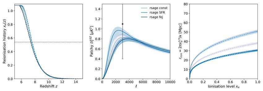
A. Gorce et al.: Improved constraints on reionisation from CMB observations: A parameterisation of the kSZ effect
redshift when reionisation ends; for patchy kSZ, the main focus bδe (k, z)2 = Pee (k, z)/Pδδ (k, z). Although coarse, this approxima-
of this work, we integrate from zend to the highest redshift consid- tion only has a minor impact on our results: it implies variations
ered in the simulation (here, zmax = 15). The contribution from of ∼ 0.05 µK2 in the power spectrum amplitude (see also Al-
redshifts larger than the onset of reionisation, when the only free varez 2016). The final expression of the power spectrum of the
electrons in the IGM are leftovers from recombination, is found curl component of the momentum field then writes
to be negligible.
We define q ≡ v(1 + δe ) = v + vδe ≡ v + qe the density-
Z
1
weighted peculiar velocity of the free electrons. It can be decom- PB,e (k, z) = f (z)2
ȧ(z)2
d3 k0 (1 − µ2 )×
(2π)3
posed into a divergence-free qB and a curl-free qE components. "
1
We write their equivalents in the Fourier domain as q̃ = q̃E + q̃B . Pee (|k − k0 |) Plinδδ (k , z)
0
As pointed out by Jaffe & Kamionkowski (1998), when pro- k02
bδe (k0 , z)
#
jected along the line of sight, q̃E will cancel and only the com-
ponent of q̃ perpendicular to k, that is q̃B , will contribute to the − bδe (|k − k |, z) Pδδ (|k − k |, z) Pδδ (k , z) ,
0 lin 0 lin 0
|k − k0 |2
kSZ signal. We want an expression for the kSZ angular power
(7)
2
spectrum C`kSZ ≡ T CMB |δT
˜ kSZ (k)|2 where k ≡ `/η is the Limber
wave-vector and ` is the multipole moment, which can be related which we can plug into Eq. (2) to find the final expression for
to an angular scale in the sky. In the small angle limit, the kSZ the kSZ angular power spectrum.
angular power spectrum can be derived from Eq. (1) using the
Limber approximation:
2.2. The power spectrum of free electrons density contrast
8π2 σ2T n̄e (z)2 2
Z
dη
C` = ∆B,e (`/η, z) e−2τ(z) η dz, (2) In Shaw et al. (2012), the authors choose to describe the be-
(2` + 1) c
3 2 (1 + z) 2 dz haviour of the free electrons power spectrum in terms of a biased
matter power spectrum: they take Pee (k, z) ≡ bδe (k, z)2 Pδδ (k, z)
with ∆2B,e (k, z) ≡ k3 PB,e (k, z)/(2π2 ) and PB,e the power spec-
and calibrate bδe (k, z) on their simulations, either extrapolating
trum of the curl component of the momentum field defined by
or assuming a reasonable behaviour for the scales and redshifts
(2π)3 PB,e δD (k − k0 ) = hq̃B,e (k) q̃∗B,e (k0 )i where δD is the Dirac
not covered by the simulations. However, because Pee describes
delta function, the tilde denotes a Fourier transform and the as-
the free electrons density fluctuations, it has a relatively simple
terisk a complex conjugate.
structure, close to the power spectrum of a field made of ionised
Expanding hq̃B,e q̃∗B,e i, we obtain:
spheres on a neutral background, shown in Fig. 1, and using a
Z 3 0
dk bias is not necessary.
q̃B,e (k) = (k̂0 − µk̂) ṽ(k0 ) δ̃e |k − k0 | , Consider a box of volume V = L3 filled with n fully ionised
(3)
(2π)3 bubbles of radius R, randomly distributed throughout the box so
that their centres are located at ai for i ∈ {1, n}. The density of
where µ = k̂ · k̂0 , so that
free electrons in the box follows
hq̃B,e (k) q̃∗B,e (k0 )i 2π2 2 n
n̄e X |r − ai |
!
≡ ∆ (k, z) ne (r) = Θ , (8)
(2π)3 δ D (|k − k0 |) k3 B,e f i=1 R
Z
1 h
= 3
d3 k0 (1 − µ2 ) Pee (|k − k0 |) Pvv (k0 ) where Θ (x) is the Heaviside step function, n̄e is the mean num-
(2π)
ber density of electrons in the box and f the filling fraction of the
(1 − µ2 ) k0
#
− Pev (|k − k |) Pev (k ) ,
0 0 box (here, f = xe ). n̄e / f is the number of electrons in one bubble
|k − k0 | divided by its volume and, ignoring overlaps, f = 4/3πR3 n/V.
(4) Consider the electron density contrast field δe on which Pee (k, z)
is built:
where the z-dependencies have been omitted for simplicity.
n !
Pee (k, z) is the power spectrum of the free electrons density ne (r) 1X |r − ai |
fluctuations and Pev is the free electrons density - velocity δe (r) = −1= Θ − 1, (9)
n̄e f i=1 R
cross-spectrum. In the linear regime, we can write v(k) =
ik ( f ȧ/k) δ̃(k), where a is the scale factor and f the linear growth represented on Fig. 2 for one of the simulations used in this work.
rate defined by f (a) = dlnD/dlna for D the growth function. δe (r) Fourier–transforms into
With this we can compute the velocity power spectrum fully
n
from linear theory and not be limited by the simulation size and L3 X
resolution: δ̃e (k) = W(kR) e−ik·ai , (10)
n i=1
!2
ȧ f (z)
Pvv (k, z) = Plin
δδ (k, z) (5) where W is the spherical top-hat window function W(y) =
k (3/y3 ) sin y − y cos y . Using this expression, and following
where Plin Bharadwaj & Pandey (2005), the power spectrum of the electron
δδ is the linear total matter power spectrum. We also density contrast field writes:
assume for the cross-spectrum:
4 31 2
Pve (k, z) ' bδe (k, z)Pδv (k, z) =
f ȧ(z)
bδe (k, z)Plin Pee (k) = πR W (kR), (11)
δδ (k, z), (6) 3 f
k
where the bias bδe is defined by the ratio of the free elec- which has units Mpc3 . Fig. 1 gives an example of such a power
trons power spectrum over the non-linear matter power spectrum spectrum. We have generated an ionisation field made of enough
Article number, page 3 of 14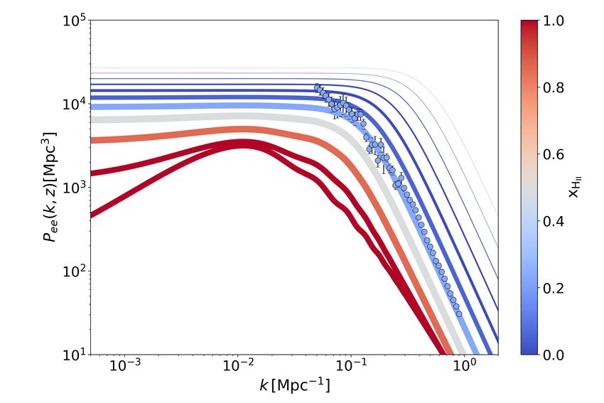
A&A proofs: manuscript no. main
process, when the variance in the free electron field is maxi-
mal (see Sec. 5.1). It then slowly decreases as xe (z)−1/5 . Be-
fore the onset of reionisation, despite the few free electrons
left over after recombination, the amplitude of Pee is negligible.
This constant power decreases above a cut-off frequency that in-
creases with time, following the growth of ionised bubbles, ac-
cording to κxe (z)−1/3 . There is no power above this frequency,
that is on smaller scales: there is no smaller ionised region than
rmin (z) = 2πxe1/3 /κ at this time. For empirical reasons, we choose
the power to decrease as k−3 and not k−4 as seen in the theo-
retical power spectrum on small scales. This difference can be
explained by the fact that in our simulations, small ionised re-
gions will keep appearing as new sources light up, maintaining
power on scales smaller than the typical bubble size. Addition-
ally, the density resolution will allow correlations between re-
gions within a given bubble, whereas in the toy models ionised
Fig. 1. Free electrons density contrast power spectrum for a box filled bubbles are only filled with ones. The complexity of the electron
with enough bubbles of radius R = 15 px = 5.5 Mpc to reach a filling density contrast field is illustrated for one of the six simulations
fraction f = 1%. Points are results of a numerical computation of the used in this work on Fig. 2: the underlying matter field is visible
power spectrum, compared to the theoretical model (solid line). The within the ionised regions.
dotted vertical line corresponds to k = 1/R, the dashed vertical line to Once reionisation is over and all IGM atoms are ionised, the
91/4 /R, the dashed horizontal line to 4/3πR3 / f and the tilted dashed line
fluctuations in free electrons density follow those of dark matter
has slope k−4 .
on large scales (k < 1 Mpc−1 ). On smaller scales, gas thermal
pressure induces a drop in Pee (k, z) compared to the dark mat-
bubbles of radius R = 15 px = 5.5 Mpc5 to reach a fill- ter. To describe this evolution at low redshifts, we choose the
ing fraction f = 1% in a box of 5123 pixels and side length same parameterisation as Shaw et al. (2012), given in Eq. (14),
L = 128/h Mpc. We compare the expression in Eq. (11) with to describe the gas bias bδe (k, z)2 = Pee (k, z)/Pδδ (k, z) but adapt
power spectrum values computed directly from the 3D field and the parameters to our simulations, which however do not cover
find a good match. On very small or very large scales, the win- redshifts lower than 5.5:
" #
dow function behaves as: 1 −k/k f 1
bδe (k, z)2 = e + . (14)
2 1 + (gk/k f )7/2
3 y3
W(y) ∼ × =1 as y → 0
y3 3 We find k f = 9.4 Mpc−1 and g = 0.5, constant with redshift.
(12) Our values for k f and g are quite different from those obtained
3 3
W(y) ∼ 3 × y = 2 as y → ∞ by Shaw et al. (2012), as in their work power starts dropping
y y between 0.05 and 0.5 Mpc−1 compared to k ∼ 3 Mpc−1 for our
simulations. This can be explained by our simulations making
so that Pee (k) ∼ 4/3πR3 / f is constant (see dashed horizontal line use of adaptive mesh refinement, therefore resolving very well
on the figure) on very large scales and has higher amplitude for the densest regions, so that our spectra are more sensitive to
smaller filling fractions. On small scales, the toy model power the thermal behaviour of gas. This model, where k f and g are
spectrum decreases as k−4 (see tilted dashed line on the figure). constant parameters, is a very basic one. It will however be suf-
The intersection point of the horizontal and tilted dashed lines ficient for this work since we focus on the patchy component
on the figure corresponds to k = 91/4 /R (dashed vertical line), of the kSZ effect, at z ≥ 5.5. Additionally, as shown later, the
hinting at a relation between the cut-off frequency and the bubble scales mostly contributing to the patchy kSZ signal correspond
size. Interestingly, Xu et al. (2019) find a similar feature, also to modes 10−3 < k/Mpc−1 < 1 where Pee follows the matter
related to the typical bubble size, in the bias between the H i and power spectrum, so that a precise knowledge of bδe (k, z) is not
matter fields. required. In the future, if we want to apply our results to con-
This behaviour is close to what we observe in the free elec- strain reionisation with the measured CMB temperature power
trons density power spectra of the custom set of simulations used spectrum, we will need a better model as the observed signal
in this work in the early stages of reionisation, as can be seen on will be the sum of homogeneous and patchy kSZ, with the for-
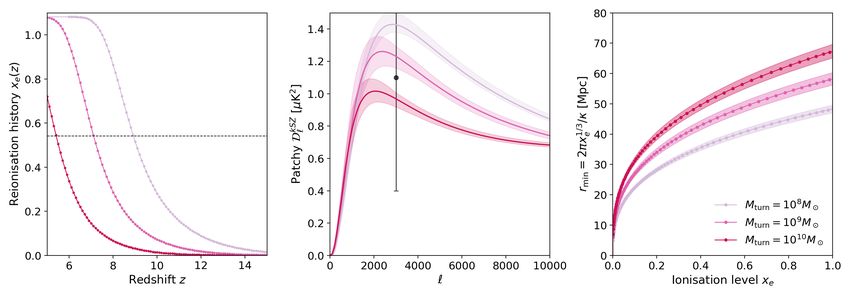
the right panel of Fig. 2. Therefore, we choose in this work to mer dominating on all scales.
use a direct parameterisation of the scale and redshift evolution To account for the smooth transition of Pee from a power-law
of Pee (k, z) during reionisation and calibrate it on our simula- to a biased matter power spectrum, illustrated in the right panel
tions. The parameters, α0 and κ, are defined according to: of Fig. 2, we write the final form for the free electrons density
fluctuations power spectrum as
α0 xe (z)−1/5
Pee (k, z) = . (13) α0 xe (z)−1/5
1 + [k/κ]3 xe (z) Pee (k, z) = fH − xe (z) ×
1 + [k/κ]3 xe (z) (15)
In log-space, on large scales, Pee has a constant amplitude which, + xe (z) × bδe (k, z)2 Pδδ (k, z),
as mentioned above, depends on the filling fraction and there-
fore reaches its maximum α0 at the start of the reionisation for fH = 1 + Y p /4X p ' 1.08, with Y p and X p the primordial mass
fraction of helium and hydrogen respectively. The total matter
5
The bubble radii actually follow a Gaussian distribution centred on power spectrum Pδδ is computed using the Boltzmann integra-
15 px with standard deviation 2 px. tor CAMB (Lewis et al. 2000; Howlett et al. 2012) for the linear
Article number, page 4 of 14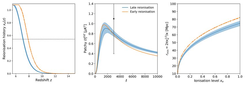
A. Gorce et al.: Improved constraints on reionisation from CMB observations: A parameterisation of the kSZ effect

Fig. 2. Left panel: Snapshot of the electron density contrast field for the first of the six simulations, at z = 7.2 and xe = 0.49. Right panel: Free
electrons power spectrum of the same simulation at fixed redshifts (fixed ionised levels). The shaded area corresponds to scales contributing Dpatchy
                                                                                                                                                 3000
the most (see Sec. 3.2) and the solid black line to the field shown in the left panel.

terms and the HALOFIT procedure for the non-linear contribu-                Table 1. Characteristics of the six high resolution simulations used. zre
tions (Smith et al. 2003).                                                  is the midpoint of reionisation xe (zre ) = 0.5 fH , zend the redshift at which
                                                                            xe (z) (extrapolated) reaches fH and τ is the Thompson optical depth. ∆z
                                                                            corresponds to z0.25 − z0.75 .

3. Calibration on simulations                                                                           zre     zend       τ xe       ∆z
                                                                                             1         7.09     5.96     0.0539      1.17
3.1. Description of the simulations                                                          2         7.16     5.92     0.0545      1.19
                                                                                             3         7.16     5.67     0.0544      1.16
     The simulations we use in this work were produced with the                              4         7.05     5.60     0.0532      1.16
EMMA simulation code (Aubert et al. 2015) and previously used                                5         7.03     5.56     0.0531      1.15
in Chardin et al. (2019). The code tracks the collisionless dynam-                           6         7.14     5.79     0.0543      1.16
ics of dark matter, the hydrodynamics of baryons, star formation                            Mean       7.10     5.84     0.0541      1.16
and feedback, and the radiative transfer using a moment-based
method (see Aubert et al. 2018; Deparis et al. 2019). This code
adheres to an Eulerian description, with fields described on grids,         computers, using CPU architectures : a reduced speed of light of
and enables adaptive mesh refinement techniques to increase the             0.1c has been used to reduce the cost of radiative transfer.
resolution in collapsing regions. Six simulations with identical                 Table 1 gives the midpoint zre and end of reionisation zend for
numerical and physical parameters were produced in order to                 each simulation, as well as the duration of the process, defined
make up for the limited physical size of the box and the associ-            as the time elapsed between global ionisation fractions of 25%
ated sample variance. They only differ in the random seeds used             and of 75%6 . The upper panel of Fig. 5 shows the interpolated
to generate the initial displacement phases, resulting in 6 differ-         reionisation histories, where data points correspond to the snap-
ent configurations of structures within the simulated volumes.              shots available for each simulation. Originally, our simulations
Each run has a (128 Mpc/h)3 volume sampled with 10243 cells                 do not include the first reionisation of helium. We correct for this
at the coarsest level and 10243 dark matter particles. Refinement           by multiplying the IGM ionised fraction of hydrogen xH ii mea-
is triggered when the number of dark matter particles exceeds 8,            sured in the simulations by fH = 1 + Y p /4X p ' 1.08. Because
up to 6 refinement levels. Initial conditions were produced using           we limit our study to redshifts z > 5.5, the second reionisation
MUSIC (Hahn & Abel 2013) with a starting redshift of z = 150,               of helium is ignored. Fig. 2 shows the electron density contrast
assuming Planck Collaboration et al. (2016a) cosmology. Simu-               field for the first of our six simulations, close to the midpoint of
lations were stopped at z ∼ 6, before the full end of reionisation.         reionisation. The complexity of the structure of this field is sum-
The dark matter mass resolution is 2.1 × 10⁸ M and the stellar              marised in its power spectrum, shown in the right panel. Fig. 3
mass resolution is 6.1 × 10⁵ M . Star formation proceeds accord-            compares the Pee (k, z) spectra of the six simulations, taken either
ing to standard recipes described in Rasera & Teyssier (2006),              at fixed redshift (first column) or fixed scale (right column). De-
with an overdensity threshold equal to 20 to trigger the gas-               spite identical numerical and physical parameters and very sim-
to-stellar particle conversion with a 0.1 efficiency: such values           ilar reionisation histories, the six simulations have different free
allow the first stellar particles to appear at z ∼ 17. Star par-            electrons density power spectra, which translates into different
ticles produce ionising radiation for 3 Myr, with an emissivity             kSZ power spectra.
provided by the Starburst99 model for a Top-Heavy initial mass
function and a Z = 0.001 metallicity (Leitherer et al. 1999). Su-
pernova feedback follows the prescription used in Aubert et al.             3.2. Calibration procedure
(2018): as they reach an age of 15 million years, stellar particles             We simultaneously fit the power spectra of the six simula-
dump 9.8 × 10¹¹ J per stellar kg in the surrounding gas, 1/3 in             tions to Eq. (15) on a scale range 0.05 < k/Mpc−1 < 1.00
the form of thermal energy, 2/3 in the form of kinetic energy. Us-          (20 bins), corresponding to the scales which contribute the most
ing these parameters, we obtain a cosmic star formation history             to the signal at ` = 3000 (see next paragraph), and a redshift
consistent with constraints by Bouwens et al. (2015) and end up
with 20 millions stellar particles at z = 6. The simulations were            6
                                                                               Some of our simulations end before reionisation is achieved, there-
produced on the Occigen (CINES) and Jean-Zay (IDRIS) super-                 fore we extrapolate xe (z) to find the zend value.

                                                                                                                           Article number, page 5 of 14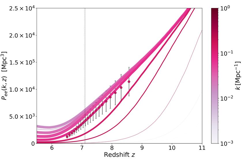
A&A proofs: manuscript no. main

Fig. 3. Result of the fit of Eq. (15) on the free electrons power spectrum of our six simulations, for three redshift bins (left panels) and three
scale bins (right panels). The best-fit is shown as the thick black line with the accompanying 68% confidence interval, and the spectra of the six
simulations as thin coloured lines. Error bars on data points are computed from the covariance matrix (see text for details).

range of 6.5 ≤ z ≤ 10.0 (10 bins), corresponding to the core                    value of 1.058 . The best-fit values, with their 68% confidence
of the reionisation process (0.07 < xe < 0.70).7 We sample the                  intervals are
parameter space of α0 and κ on a regular grid (with spacings
                                                                                log α0 /Mpc3 = 3.93+0.05
∆ log α0 = 0.001 and ∆κ = 0.0001) for which we compute the                                         −0.06
                                                                                                                                              (17)
following likelihood:                                                           κ = 0.084+0.003
                                                                                         −0.004 Mpc .
                                                                                                   −1

        6 XX                                                                    We note a strong correlation between the two parameters due to
       X       1 h data                               i2
                                                                                both physical – see Sec. 5.1 – and analytical reasons. Indeed, the
χ2 =              Pee (k j , zi ) − Pmodel (k j , zi ) ,               (16)
       n=1 z k
               σe
                2                    ee
                                                                                value of κ impacts the low-frequency amplitude of the Pee (k, z)
             i   j
                                                                                model. The best-fit model, compared to the Pee (k, z) spectra of
where {zi } and {k j } are the redshift and scale bins and the first            the six simulations Eq. (15) is fitted on, can be seen in Fig. 3
sum is over the six simulations. Because our sample of six simu-                for three different redshift bins (left-hand column) and three dif-
lations is not sufficient to derive a meaningful covariance matrix,             ferent scale bins (right-hand column). Overall, we see a good
we choose to ignore correlations between scales across redshifts                agreement between the fit and the data points on the scales of
and use the diagonal of the covariance matrix to derive error bars              interest, despite the simplicity of our model.
σe for each data point. We refer the interested reader to a dis-                    Given the large number of Pee (k, z) data points originally
cussion of this choice in Appendix A. We choose the best-fit as                 (∼ 3500) and the complexity of the evolution of Pee with k and
the duplet (α0 , κ) for which the reduced χ2 reaches its minimum                z, we must limit our fits to given ranges. In order to assess what
                                                                                scales and redshifts contribute the most to the final kSZ signal,
 7                                                                              we look at the evolution of the integrand on z in Eq. (2) with
   Because the snapshots of each simulation are not taken at the same
redshifts or ionisation levels, we interpolate Pee (k, z) for each simulation   time and at the evolution of the integral on k in Eq. (7) with
and then compute the interpolated spectra for a common set of ionisa-           scales. The results are shown in Fig. 4. The left (resp. right) up-
tion levels, with less elements than the original number of snapshots.          per panel presents the evolution of Pee (k, z) with scales (resp.
Note that the original binning in scales for Pee (k, z) is the same for the
six simulations but reduced from 38 to 20 bins.                                 8
                                                                                    The raw value is χ2 ∼ 2500.

Article number, page 6 of 14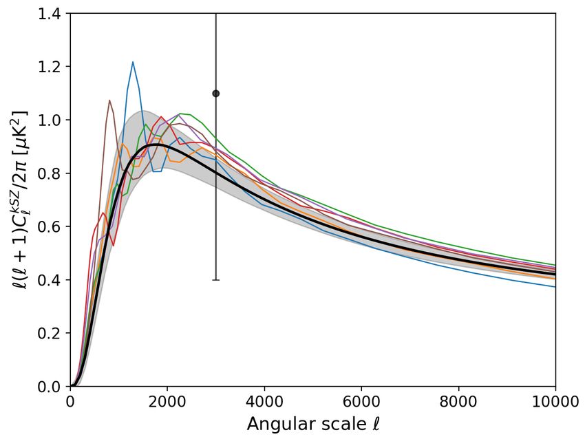
A. Gorce et al.: Improved constraints on reionisation from CMB observations: A parameterisation of the kSZ effect

Fig. 4. Upper panels: Pee (k, z) as fitted on spectra from the fourth simulation, as a function of scales (left panel) and of redshift (right panel). For
reference, the fit is compared to data points for z = 7.8 (xe = 0.26) and k = 0.14 Mpc−1 respectively, with corresponding colour. The width of
each line represents the contribution of the redshift (resp. scale) of the corresponding scale (resp. redshift) to the final patchy kSZ amplitude at
` = 3000. Lower panels: Corresponding probability densities (dashed lines) and cumulative distributions (solid lines). Shaded areas correspond to
the first 50% of the signal. The dotted vertical line on the lower right panel marks the midpoint of reionisation.

redshift) after applying the fitting procedure described above.               power spectrum is shown on the lower panel of Fig. 5. The er-
The width of each line represents the contribution of the red-                ror bars correspond to the propagated 68% confidence interval
shift (resp. scale) of the corresponding colour to the final patchy           on the fit parameters. The amplitude of the homogeneous sig-
kSZ amplitude at ` = 3000. The lower panels present the cor-                  nal largely dominates that of the patchy signal, being about 4
responding probability density and cumulative distribution func-              times larger. The total kSZ amplitude reaches D3000 = 4.2 µK2
tions. We find that redshifts throughout reionisation contribute              and so slightly exceeds the upper limits on the total kSZ am-
homogeneously to the signal, since 50% stems from redshifts                   plitude given by SPT and Planck when SZxCIB correlations are
z ≤ 7.2, slightly before the midpoint zre = 7.0. Redshifts on the             allowed (resp. Reichardt et al. 2020; Planck Collaboration et al.
range 6.5 < z < 8.5 contribute the most as they represent about               2016b) but is however within the error bars of the ACT results
75% of the final kSZ power. Conversely, redshifts z > 10 con-                 (Sievers et al. 2013). With respect to the patchy signal, the am-
tribute to only 0.4% of the total signal. On the lower panel, we              plitude is in perfect agreement with the claimed detection by the
see that scales outside the range 10−3 Mpc−1 < k < 1 Mpc−1 con-               SPT at D3000 = 1.1+1.0
                                                                                          patchy
                                                                                                      −0.7 µK (Reichardt et al. 2020), noting that
                                                                                                             2
tribute very marginally to the final signal (about 0.2%), whereas             our simulations reionise in a time very close to their constraint
the range 10−2 < k/Mpc−1 < 10−1 makes up about 70% of                         ∆z = 1.1+1.6
                                                                                         −0.7 . The spectrum exhibits the expected bump in am-
D3000 . Therefore, we choose to only keep data within the red-                plitude, here around ` ∼ 1800, corresponding to larger scales
shift range 6.5 < z < 10.0 (i.e. 7% < xe < 70%) and the scale                 than those found in other works (Iliev et al. 2007; Mesinger
range 10−3 < k/Mpc−1 < 1 to constrain our fits. For reference,                et al. 2012), hinting at larger ionised bubbles on average. Fig. 5
on Fig. 4, we compare the fit to data points at z = 7.8 (xe = 0.26)           gives an idea of the variance in the kSZ angular power spectrum
and k = 0.14 Mpc−1 for the first simulation, and find an overall              for given physics – in particular a given matter distribution, and
good match.                                                                   very similar reionisation histories: the distribution among simu-
                                                                              lations gives a reionisation midpoint defined at zre = 7.10 ± 0.06,
                                                                              corresponding to a range of kSZ power spectrum amplitude
4. Propagation to the kSZ power spectrum                                      D3000 = 0.80 ± 0.06 µK2 (at 68% confidence level). Part of
4.1. Results on our six simulations                                           this variance can be related to sample variance, since our sim-
                                                                              ulations have a too small side length (L = 128 Mpc/h) to avoid
   Now that we have a fitted Pee (k, z), we can compute the kSZ               it (Iliev et al. 2007). We compare in Fig. 5 the kSZ power spec-
angular power spectrum using Eq. (2). We find:                                trum resulting from fitting Eq. (15) on our six simulations si-
  p                                                                           multaneously to the six spectra obtained when interpolating the
D3000 = 0.80 ± 0.06 µK2                                              (18)
                                                                              Pee (k, z) data points available for each simulation: the six inter-
and the angular scale at which the patchy angular spectrum                    polated spectra lie withing the confidence limits of our best-fit.
reaches its maximum is `max = 1800+300
                                   −100 . The angular patchy

                                                                                                                          Article number, page 7 of 14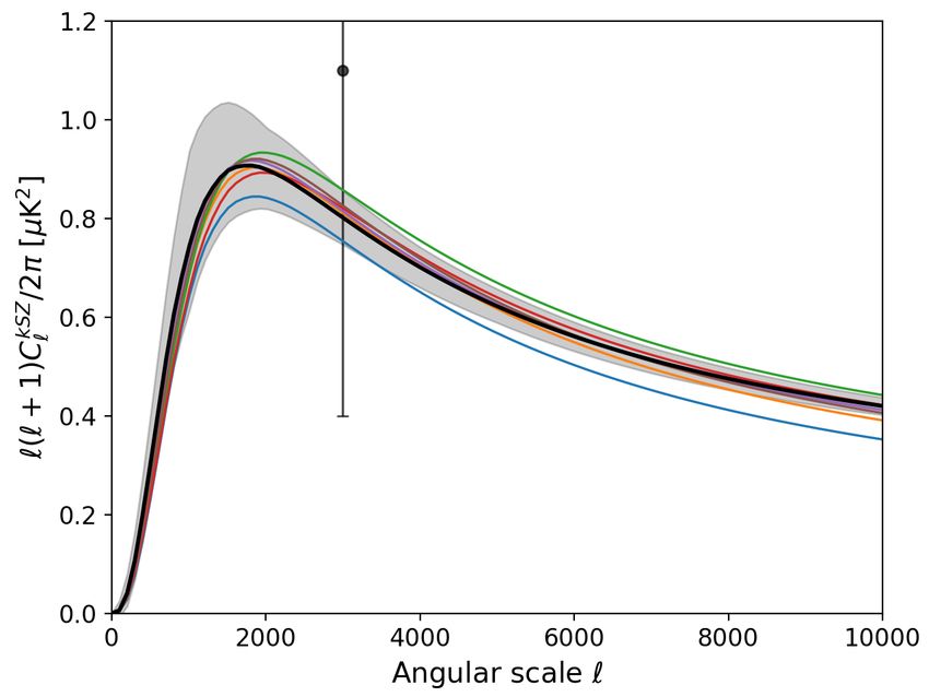
A&A proofs: manuscript no. main

Fig. 5. Results for our six simulations. Upper panel: Global reionisa-          Fig. 6. Evolution of the amplitude of the patchy power spectrum at
tion histories, for H ii and He ii. The dotted horizontal line marks the        ` = 3000, D3000 with the reionisation duration (upper panel) and the
reionisation midpoint zre . Lower panel: Angular kSZ power spectrum             reionisation midpoint zre (lower panel), for different values of our pa-
after fitting Eq. (15) to the Pee (k, z) data points from our six simulations   rameters. Error bars correspond to the dispersion of kSZ amplitude at
(thick solid line) compared to the spectra obtained when interpolating          ` = 3000 (68% confidence level) propagated from errors on the fit pa-
the data points for each simulation (thin solid lines). Error bars cor-         rameters. The diamond data point corresponds to a seventh simulation,
respond to the propagation of the 68% confidence interval on the fit            with reionisation happening earlier. In both panels, results are compared
parameters. The data point corresponds to constraints from Reichardt            to those of Battaglia et al. (2013), rescaled to our cosmology.
et al. (2020) at ` = 3000.

                                                                                twice as much star formation as in the six initial simulations,
    Fixing the fit parameters to their most likely value for the
                                                                                therefore reionising earlier (zre = 7.94) but on a similar redshift
fourth simulation, we artificially vary the reionisation history
                                                                                interval (∆z = 1.20). Applying the fitting procedure described
and compute the corresponding power spectrum. We succes-
                                                                                above, we find logα0 = 4.10 and κ = 0.08 Mpc−1 . The resulting
sively fix the reionisation redshift but increase its duration ∆z
                                                                                patchy kSZ power spectrum can be seen in Fig. 7, along with
or fix the duration but shift the midpoint zre . This corresponds
                                                                                the reionisation histories and the evolution of the typical bubble
to a scenario where the reionisation morphology is exactly the
                                                                                size rmin = 2π/κxe (z)1/3 . Results for this simulation are com-
same, but happens later or earlier in time. We find clear scal-
                                                                                pared with what was obtained for our six simulations. The kSZ
ing relations between the amplitude of the signal at ` = 3000,
                                                                                spectrum corresponding to an early reionisation scenario bumps
D3000 , and both the reionisation duration ∆z and its midpoint zre .
                                                                                at larger scales (`max = 1400) with a much larger maximum am-
However, they are sensibly different from the results of Battaglia
                                                                                plitude (Dmax = 0.98 µK2 ) but interestingly the amplitudes at
et al. (2013) as can be seen in Fig. 6. Even after rescaling to their
                                                                                ` = 3000 are similar. This suggests that focusing on D3000 is not
zre = 8 and cosmology, we get a much lower amplitude. Note
                                                                                sufficient to characterise the kSZ signal.
also that their patchy spectra bump around ` = 3000, whereas
in our simulations the power has already dropped by ` = 3000                        These results corroborate the work of Park et al. (2013), who
(Fig. 5), hinting at a very different reionisation morphology from              found that the scalings derived in Battaglia et al. (2013) are
ours. When we vary κ and α0 artificially, by fixing logα0 = 3.54                largely dependent on the simulations they were calibrated on,
instead of 3.70 as before, there is still a scaling relation, but               and therefore cannot be used as a universal formula to constrain
both the slope and the intercept change. All of this demonstrates               reionisation. Notably, an asymmetric reionisation history xe (z)
that the amplitude of the patchy signal largely depends on the                  naturally deviates from this relation. Global parameters such as
physics of reionisation (here via the κ and α0 parameters) and                  ∆z and zre are not sufficient to accurately describe the patchy kSZ
∆z and zre are not sufficient to derive D3000 . Simulations closer              signal, and one needs to take the physics of reionisation into ac-
to those used in Battaglia et al. (2013) would likely give larger               count to get an accurate estimation of not only the shape, but
values for κ and α0 , therefore increasing the amplitude to val-                also the amplitude of the power spectrum. Additionally, limiting
ues closer to the authors’ results. To confirm this, we generate                ourselves to the amplitude at ` = 3000 to constrain reionisation
a new simulation, with same resolution and box size but with                    can be misleading.
Article number, page 8 of 14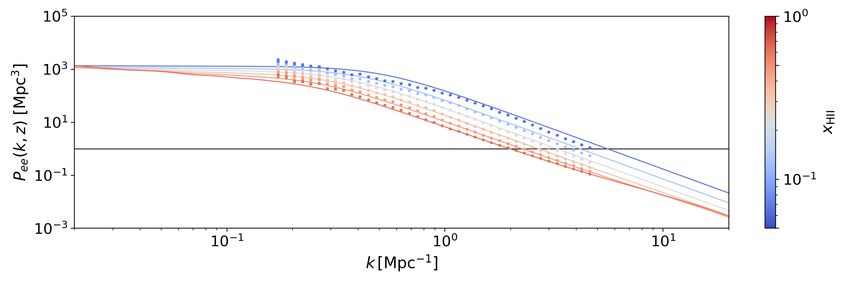
A. Gorce et al.: Improved constraints on reionisation from CMB observations: A parameterisation of the kSZ effect

Fig. 7. Comparison of results for our six initial simulations, corresponding to a late reionisation scenario, and for an additional seventh simulation,
corresponding to an early reionisation scenario. Left panel: Reionisation histories. Middle panel: Patchy kSZ angular power spectra. The data
point corresponds to constraints from Reichardt et al. (2020). Right panel: Minimal size of ionised regions as a function of global ionised level.
Shaded areas correspond to the 68% confidence level on kSZ amplitude propagated from the probability distributions of the fit parameters.

4.2. Tests on other simulations                                              of the ne (r) field. Therefore a smaller α0 value is equivalent to
                                                                             a smaller field variance at all times. This is consistent with the
                                                                             picture of the different rsage simulations we have: as presented
     We now look at the rsage simulation, described in Seiler                in Seiler et al. (2019), rsage fej exhibits the smallest ionised
et al. (2019), to test the robustness of our parameterisation.               bubbles on average. For a given filling fraction, a field made of
This simulation starts off as an N-body simulation (Seiler et al.            many small bubbles covering the neutral background rather ho-
2018), containing 24003 dark matter particles within a 160 Mpc               mogeneously will have smaller variance than one made of a few
side box, resolving halos of mass ∼ 4 × 10⁸ M with 32 par-                   large bubbles. This in turn explains why rsage SFR gives the
ticles. Galaxies are evolved over cosmic time following the                  largest α0 value (log α0 = 3.47 ± 0.04), and, later, the largest
Semi-Analytic Galaxy Evolution (SAGE) model of Croton et al.                 kSZ amplitude (Fig. 8). Second, the rsage SFR simulation has
(2016), modified to include an improved modelling of galaxy                  the smallest value of κ (κ = 0.123±0.004 Mpc−1 ): the upper right
evolution during the Epoch of Reionisation, including the feed-
back of ionisation on galaxy evolution. The semi-numerical                   panel of Fig. 8 shows the evolution of rmin = 2π/κxe1/3 with ion-
code cifog (Hutter 2018a,b) is used to generate an inhomoge-                 isation level for the three models. Because rsage SFR has the
neous ultraviolet background (UVB) and follow the evolution of               largest ionised bubbles on average (Seiler et al. 2019), this result
ionised hydrogen during the EoR. Three versions of the rsage                 confirms the interpretation of 1/κ as an estimate of the typical
simulation are used, each corresponding to a different way of                bubble size during reionisation. Additionally, the patchy power
modelling the escape fraction fesc of ionising photons from their            spectrum derived from rsage SFR peaks at larger angular scales
host galaxy into the IGM. The first, dubbed rsage const, takes               (`max ∼ 2400) than for the other simulations, as can be seen in
 fesc constant and equal to 20%. The second, rsage fej, con-                 the upper middle panel of the figure. Interestingly, the largest α0
siders a positive scaling of fesc with fej , the fraction of baryons         value leads to the strongest kSZ signal and the smallest κ value to
that have been ejected from the galaxy compared to the num-                  the spectrum whose bump is observed on the largest scales (the
ber remaining as hot and cold gas. In the last one, rsage SFR,               smallest `max ). We investigate these potential links in the next
 fesc scales with the star formation rate and thus roughly with              section.
the halo mass. Because they are based on the same dark mat-                      We now turn to three 21CMFAST (Mesinger & Furlan-
ter distribution, the three simulations start reionising at simi-            etto 2007; Mesinger et al. 2011) simulations with dimensions
lar times (z ∼ 13), but different source properties lead to dif-             L = 160 Mpc for 2563 cells (same box size and resolution as
ferent reionisation histories, shown in the left upper panel of              rsage). Between the three runs, we vary the parameter Mturn ,
Fig. 8. In rsage SFR, the ionised bubbles are statistically larger           the turnover mass, which corresponds to the minimum halo mass
than the other two simulations at a given redshift: this results             before exponential suppression of star formation. For Mturn =
into rsage SFR reaching 50% of ionisation at zre = 7.56 vs.                  108 M , the box is fully ionised by zend = 6.25 and the mid-
zre = 7.45 and zre = 7.37 for rsage const and rsage fej                      point of reionisation is reached at zre = 8.92 for a process lasting
respectively, and the full ionisation being achieved in a shorter            ∆z = 1.91. For Mturn = 109 M , we find zend = 4.69, zre = 7.11
time. For more details, we refer the interested reader to Seiler             and ∆z = 1.66, which is closest to rsage and our initial six sim-
et al. (2019). Applying the fitting procedure to the three simula-           ulations. Finally, Mturn = 1010 M yields zend = 3.37, zre = 5.41
tions, we find that the parameterisation of Eq. (15) is an accurate          and ∆z = 1.47. Indeed, the point of these simulations is not only
description of the evolution of their Pee (k, z) spectra (detailed           to test the sensitivity of our approach to astrophysical param-
fit results are given in App. B.2). Resulting patchy kSZ angular             eters, but also to see the impact of very different reionisation
power spectra are shown in the upper middle panel of Fig. 8.                 histories on the patchy kSZ power. We find that Eq. (15) again
First, we find that rsage fej has the smallest α0 value, with                nicely fits the evolution of the Pee (k, z) spectra of these simu-
log α0 = 2.87 ± 0.04. Because α0 is the maximum amplitude of                 lations, as shown in App. B.1. The resulting reionisation his-
the Pee (k, z) spectrum, built upon the free electrons density con-          tories, patchy kSZ spectra and rmin (xe ) are shown in the lower
trast field δe (r) = ne (r)/n̄e − 1, it will scale with the variance         panels of Fig. 8. For Mturn = 108 M , many small-mass halos
                                                                                                                         Article number, page 9 of 14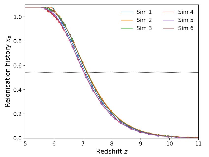
A&A proofs: manuscript no. main

Fig. 8. Comparison of results for the three rsage simulations (upper panels) and the three 21CMFAST runs (lower panels) considered. Left panels:
Reionisation histories. Middle panels: Patchy kSZ angular power spectra. The data point corresponds to constraints from Reichardt et al. (2020).
Right panels: Minimal size of ionised regions as a function of global ionised level. The shaded areas correspond to the 68% confidence interval
propagated from the 68% confidence intervals on the fit parameters.

are active ionising sources, resulting in an ionising field made         the physical interpretation of the parameters α0 and κ detailed in
of many small bubbles at the start of the process. This translates       the next Section.
into this simulation having the largest best-fit κ value of the three
(κ = 0.130 ± 0.003 Mpc−1 ) and so the smallest rmin (xe ). Natu-
rally, the resulting kSZ spectrum peaks at smaller angular scales.       5. Discussion and conclusions
For the other extreme case Mturn = 1010 M , because the minimal          5.1. Physical interpretation of the parameters
mass required to start ionising is larger, the ionising sources are
more efficient and the ionised bubbles larger. Indeed, we find a             Many previous works have empirically related the angular
smaller value of κ = 0.093 ± 0.003 Mpc−1 . With larger bubbles,          scale at which the patchy kSZ power spectrum reaches its maxi-
we also expect the variance in the ionisation field at the start of      mum `max to the typical size of bubbles during reionisation (Mc-
the process to be higher than if many small ionised regions cover        Quinn et al. 2005; Iliev et al. 2007; Mesinger et al. 2012). To test
the neutral background. This corresponds to the larger value of          for this relation, we compute the patchy kSZ power spectrum for
log α0 = 3.79 ± 0.04 found for this simulation, compared to              a given reionisation history xe (z) and α0 but let κ values vary.
3.30 ± 0.03 for the first one. However, this larger value of α0 this     We find a clear linear relation between κ and `max as shown in
time does not result into the strongest kSZ signal because of the        Fig. 9. Despite very different reionisation histories and physics
very different reionisation histories of the three simulations. As       at stake, previous results on the six high-resolution simulations,
we have seen in the previous section, the amplitude of the signal        on 21CMFAST, and on rsage, roughly lie along this line. This
is strongly correlated with the duration and midpoint of reioni-         means that a detection of the patchy power spectrum in CMB ob-
sation, resulting in the first simulation (Mturn = 108 M ), corre-       servations would make it possible to directly estimate `max , giv-
sponding to the earliest reionisation, having the strongest signal.      ing access to κ without bias from reionisation history, and to the
This again emphasises how essential it is to consider both reion-        evolution of the typical bubble size. As the growth of ionised re-
isation morphology and global history to derive the final kSZ            gions depends on the physical properties of early galaxies, such
spectrum.                                                                as their ionising efficiency or their star formation rate and on the
                                                                         density of the IGM, constraints on κ could, in turn, give con-
   These results show that our proposed simple two-parameter             straints on the nature of early light sources and of the early IGM.
expression for Pee (k, z) can accurately describe different types of         Additionally, we can link the theoretical expression of the
simulations, that is different types of physics, further validating      large-scale amplitude of the bubble power spectrum in Eq. (11)
Article number, page 10 of 14
A. Gorce et al.: Improved constraints on reionisation from CMB observations: A parameterisation of the kSZ effect
of the angular power spectrum of the kSZ effect stemming from
patchy reionisation. We have shown that describing the shape,
but also amplitude of the signal only in terms of global param-
eters such as the reionisation duration ∆z and its midpoint zre
is not sufficient: it is essential to take the physics of the pro-
cess into account. In our new proposed expression, the parame-
ters can be directly related to both the global reionisation history
xe (z) and to the morphology of the process. With as few as these
three parameters, we can fully recover the patchy kSZ angular
power spectrum, in a way that is quick and easy to forward-
model. Our formalism contrasts with current works, which use
an arbitrary patchy kSZ power spectrum template enclosing an
outdated model of reionisation. Applying it to CMB data will re-
sult in obtaining for the first time the actual shape of the patchy
kSZ power spectrum, taking consistently into account reionisa-
tion history and morphology. In future works, we will apply this
Fig. 9. Evolution of the peaking angular scale of the patchy kSZ power framework to CMB observations from SPT and, later, CMB-S4
spectrum for one given reionisation history but different values of the κ experiments. Then, the inferred values of α0 and κ will provide
parameter. The red dotted line is the result of a linear regression. Infer- us with detailed information about the physics of reionisation:
ences are compared to results for different simulations. κ will constrain the growth of ionised bubbles with time and α0
the evolution of the variance of the ionisation field during EoR,
both being related to the ionising properties of early galaxies.
with our parameterisation of Pee (k, z) in Eq. (13): α0 xe−1/5 ↔ The complex derivation of the kSZ signal, based on a series of
4/3πR3 /xe (z). Because of the simplicity of the toy model, this integrals, leads to correlations between our parameters. For ex-
relation is not an equivalence. For example, contrary to the toy ample, a high amplitude of the spectrum can be explained ei-
model, in our simulations, the locations of the different ionised ther by a large value of α0 due to a high ionising efficiency of
bubbles are correlated, following the underlying dark matter dis- galaxies, or by an early reionisation. Such degeneracies, how-
tribution and this correlation will add power to the spectrum on ever, could be broken by combining CMB data with other obser-
large scales. This analogy can however explain the correlation vations: astrophysical observations of early galaxies and quasars
observed between α0 and κ when fitting Eq. (15) to data (recall will help grasp the global history of reionisation and constrain
that R ∝ 1/κ). Finally, since α0 is independent of redshift, it parameters such as ∆z and zre , while 21cm intensity mapping
will be a pre-factor for the left-hand side of Eq. (7), therefore will help understand reionisation morphology, putting indepen-
we expect a strong correlation between this parameter and the dent constraints on α0 and κ. The main challenge remains to sep-
amplitude of the spectrum at ` = 3000 and with the maximum arate first the kSZ signal from other foregrounds, and then the
amplitude reached by the spectrum. We confirm this intuition by patchy kSZ signal from the homogeneous one. To solve the first
fixing the reionisation history and κ but varying α0 on the range part of this problem, Calabrese et al. (2014) suggest to subtract
3.0 < log α0 < 4.4 and comparing the resulting spectra: there is the theoretical primary power spectrum (derived from indepen-
a clear linear relation between these two parameters and α0 , but dent cosmological parameter constraints obtained from polarisa-
in this case results for rsage and 21CMFAST do not follow the tion measurements) from the observed one so that the signal left
correlation. Interestingly, the shape of the different resulting kSZ is the kSZ power spectrum alone. Secondly, one would need a
power spectra is strictly identical (namely, `max does not change good description of the homogeneous spectrum, similar to the
when varying α0 ), hinting at the fact that `max depends only on κ results of Shaw et al. (2012) but updated with more recent simu-
and not α0 or reionisation history. Therefore it will be possible to lations, in order to estimate how accurately one can recover the
make an unbiased estimate of κ from the shape of the measured patchy signal. Additionally, this result sheds light on the scaling
spectrum. The rsage simulations show that, for a similar reion- relations observed in previous works by giving them a physical
isation history, a larger value of α0 will lead to a stronger kSZ ground. For example, features in the free electron contrast den-
signal; but looking at 21CMFAST, we found that an early reion- sity power spectrum explain the relation between the amplitude
isation scenario can counterbalance this effect and lead to high at which the patchy kSZ spectrum bumps `max and the typical
amplitude despite low α0 values. This corroborates the results of bubble size, which was observed empirically in many previous
Mesinger et al. (2012), which find that the amplitude of the spec- works (McQuinn et al. 2005; Iliev et al. 2007; Mesinger et al.
trum is determined by both the morphology (and so the α0 value) 2012).
and the reionisation history. Therefore, fitting CMB data to our On average, our results are in good agreement with previous
parameterisation will likely lead to strongly correlated values of works, despite a low amplitude of the patchy kSZ angular power
α0 and parameters such as ∆z or zre . Other methods should be spectrum at ` = 3000 (∼ 0.80 µK2 ) for our fiducial simulations.
used to constrain the reionisation history and break this degen- There is undoubtedly a bump around scales ` ∼ 2000 that can
eracy, such as constraints from the value of the Thomson opti- be related to the typical bubble size and the amplitude of the to-
cal depth, or astrophysical constraints on the IGM ionised level. tal (patchy) kinetic SZ spectrum ranges from 4 to 5 µK2 (0.5 to
Conversely, 21cm intensity mapping should be able to give in- 1.5 µK2 , respectively) for plausible reionisation scenarios, there-
dependent constraints on α0 . fore lying within the error bars of the latest observational results
of ACT (Sievers et al. 2013) and SPT (Reichardt et al. 2020). We
5.2. Conclusions & prospects have found that the majority of the patchy kSZ signal stems from
scales 10−3 < k/Mpc−1 < 1 and from the core of the reionisation
In this work, we have used state-of-the-art reionisation sim- process (10% < xe < 80%), ranges on which we must focus our
ulations (Aubert et al. 2015) to calibrate an analytical expression efforts to obtain an accurate description. This analysis does not
Article number, page 11 of 14You can also read