Rapid three dimensional multiparametric MRi with quantitative transient state imaging - Nature
←
→
Page content transcription
If your browser does not render page correctly, please read the page content below
www.nature.com/scientificreports
OPEN Rapid three‑dimensional
multiparametric MRI
with quantitative transient‑state
imaging
Pedro A. Gómez1*, Matteo Cencini3,4, Mohammad Golbabaee5, Rolf F. Schulte6,
Carolin Pirkl1,6, Izabela Horvath1,6, Giada Fallo2,3, Luca Peretti2,3, Michela Tosetti3,4,
Bjoern H. Menze1 & Guido Buonincontri3,4
Novel methods for quantitative, transient-state multiparametric imaging are increasingly being
demonstrated for assessment of disease and treatment efficacy. Here, we build on these by assessing
the most common Non-Cartesian readout trajectories (2D/3D radials and spirals), demonstrating
efficient anti-aliasing with a k-space view-sharing technique, and proposing novel methods for
parameter inference with neural networks that incorporate the estimation of proton density. Our
results show good agreement with gold standard and phantom references for all readout trajectories
at 1.5 T and 3 T. Parameters inferred with the neural network were within 6.58% difference from the
parameters inferred with a high-resolution dictionary. Concordance correlation coefficients were
above 0.92 and the normalized root mean squared error ranged between 4.2 and 12.7% with respect
to gold-standard phantom references for T1 and T2. In vivo acquisitions demonstrate sub-millimetric
isotropic resolution in under five minutes with reconstruction and inference times < 7 min. Our 3D
quantitative transient-state imaging approach could enable high-resolution multiparametric tissue
quantification within clinically acceptable acquisition and reconstruction times.
Quantitative, multiparametric imaging offers great opportunities for assessment of disease and treatment efficacy.
Compared to contrast-weighted images, quantitative measurements are less influenced by system and interpreta-
tion biases, increasing data reproducibility and accuracy1. However, obtaining quantitative information usually
requires the acquisition of multiple views along each parameter-encoding dimension, which often leads to
impractically long scan times. To overcome this challenge, various rapid multiparametric mapping techniques
have recently been demonstrated2–5. Compared to methods for estimating a single parameter at a time, the
models at the heart of these techniques have the main advantage of accounting for the correlations between all
quantitative parameters of interest as well as system imperfections. This holistic view of the MR signal enables
the simultaneous regression of many individual parameters, potentially with higher accuracy. Novel, accurate
techniques promise a fast estimation of relevant MRI quantities, including but not limited to, the longitudinal
(T1) and transverse (T2) relaxation times, allowing also retrospective synthesis of conventional MR c ontrasts3.
Amongst these emerging methods, MR Fingerprinting (MRF)2, quantitative transient-state imaging (QTI)4,
and Magnetic Resonance Spin TomogrAphy in Time-domain (MR-STAT)5, are currently being demonstrated
in healthy subjects and/or patient groups.
These quantitative techniques, following the seminal paper by Ma et al.2, use similar strategies to simultane-
ously sample the k-space and parameter space, relying on transient-state6 acquisitions achieved by continuous
variations of the acquisition parameters while acquiring undersampled k-space snapshots after each excitation.
Parametric maps are subsequently computed by enforcing consistency with a physical model, i.e. the Bloch equa-
tions. While these methods have been shown to be robust to aliasing artifacts, extreme undersampling factors
may still lead to quantification errors and decreased image quality. The local quantification accuracy depends both
on the used flip angle schedule and the k-space sampling trajectory, as time-dependent point spread functions
1
Computer Science, Munich School of Bioengineering, Technical University of Munich, Munich,
Germany. 2University of Pisa, Pisa, Italy. 3Imago7 Foundation, Pisa, Italy. 4IRCCS Stella Maris, Pisa, Italy. 5University
of Bath, Bath, UK. 6GE Healthcare, Munich, Germany. *email: pedro.gomez@tum.de
Scientific Reports | (2020) 10:13769 | https://doi.org/10.1038/s41598-020-70789-2 1
Vol.:(0123456789)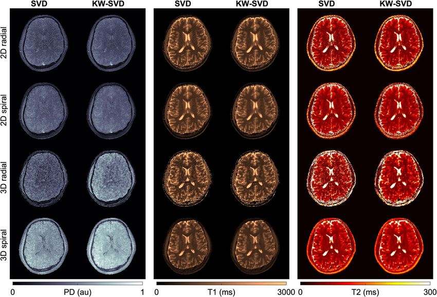
www.nature.com/scientificreports/
(PSF) will interfere differently in different spatiotemporal coordinates7. So far, the most successful implementa-
tions of transient-state imaging have relied on trajectories that oversample the k-space center, such as radial or
spiral acquisitions, in combination with locally-smooth schedules of flip angle and repetition t imes8,9. Despite
their initial success in high-resolution parameter mapping, current quantitative techniques still suffer from
limitations in acquisition, reconstruction, and parameter inference efficiency.
Multiple studies have been presented to address acquisition shortcomings. For example, three-dimensional
readouts have been applied—either as stack-of-spirals7,10, 3D spiral projections11, or music-based k-space
trajectories12—reaching whole-brain high-resolution parameter mapping in clinically feasible acquisition times.
Other works have focused on optimizing the flip angle schedule for efficient parameter sampling using Bayesian
experimental design4 or Crámer-Rao Lower B ound9,13,14. These optimization works generally converge to smooth
transient-state signal evolutions, enabling the replacement of brute-force dictionary matching with voxel-wise
fitting15,16, as smooth signal evolutions avoid local minima in the Bloch-response manifold17.
Accelerated acquisitions have been combined with advanced reconstruction algorithms and parameter
inference techniques to ameliorate quantification errors associated with aliasing and noise due to increased
undersampling. Simple, non-iterative methods, such as sliding window reconstruction7,11,18 or k-space weighted
view-sharing19,20 have demonstrated improved quantification accuracy over traditional linear matrix inversion.
Moreover, iterative algorithms further reduce quantification errors by imposing low-rank subspace constraints
on either temporal signals or spatial image models4,21–25. Advanced reconstructions, however, generally trade-
off shorter scan durations against increased computing times, hindering their clinical applicability. Finally,
machine learning algorithms have demonstrated improved parameter inference; for instance, by either learning
the dictionary26,27 or completely replacing it with artificial neural n etworks28–30. The latter approach also tackles
dictionary discretization and size limitations, enabling higher-dimensional applications of multiparametric map-
ping, such as capturing the full diffusion tensor together with relaxation p arameters29.
This work focuses on 3D acquisition, reconstruction, and parameter inference for multiparametric mapping
of the brain. Our contributions are summarized as follows:
1. We provide a systematic comparison of the most common non-Cartesian readout trajectories, namely 2D/3D
spiral arms and radial spokes. We compare them in terms of efficiency, coverage, PSF, and impact on quanti-
fication accuracy; showing that 3D spirals achieve the most efficient coverage for whole brain quantification.
2. To overcome computation and memory-expensive dictionary matching approaches, we employ a novel
compact artificial neural network for parametric inference in a lower dimensional subspace. Along with the
prediction of T1 and T2 relaxation times, we include the quantification of proton density (PD) as a linear
scaling factor into the neural network setup.
3. We demonstrate a reduction in reconstruction time for 3D high-resolution mapping from 1.5 to 4 h ours11
to under 7 min.
Methods
Data acquisition and reconstruction with non‑Cartesian readout trajectories. Sequence pa‑
rameters. Data acquisition is performed during the transient-state, with varying acquisition parameters from
one repetition to the next. Repetition time (TR) and echo time (TE) were chosen to be constant and minimal
throughout the experiment, resulting in TR = 10.5/12 ms (for 3 T/1.5 T, respectively) and TE = 0.46/2.08 ms (for
spiral/radial acquisitions, respectively). The unbalanced gradient was designed to achieve a 4π dephasing over
the z direction of the voxel. The choice of the variable acquisition parameters is shown in Fig. 1. As described
by previous work4, the inversion pulse followed by the increasing flip angle ramp encodes simultaneously for T1
and T24. The decreasing ramp will then smoothly reduce the magnetization until the last section of the flip angle
train. This portion with a small and constant flip angle, in turn, allows for T1 recovery before the next inversion
pulse. It also allows to repeat the acquisition obtaining full 3D encoding. We call these repetitions segments, as
opposed to the repetitions of the excitations.
For the readout trajectory, we implemented and evaluated the most common non-Cartesian readout tra-
jectories: 2D/3D spiral and radial readouts. Each readout is compared in terms of PSF and sampling efficiency.
Readout trajectories. All readout trajectories were based on rotations of an individual fundamental interleave:
2D radial. A full-spoke radial readout was rotated by a golden angle within each TR, covering a fully sampled
disk during the whole acquisition schedule.
2D spiral. The fundamental waveform consisted of a variable density spiral interleave implemented using
esign31. This waveform was rotated by a golden angle within each TR as in
time-optimal gradient waveform d
the 2D radial case.
3D radial. The same full-spoke radial readout used for 2D radial trajectory was rotated both around the z-axis
(in-plane rotations) and the x-axis (spherical rotations) to cover a 3D volume of the k-space. A pseudo-random
order of the spokes was achieved by random permutation of the readout order. The acquisition was performed
using this ordering and using a single interleave within each TR.
3D spiral. The same variable-density spiral interleave used to construct 2D spiral trajectory was rotated along
two different angles: in-plane rotations and spherical rotations. Full in-plane k-space coverage was achieved
Scientific Reports | (2020) 10:13769 | https://doi.org/10.1038/s41598-020-70789-2 2
Vol:.(1234567890)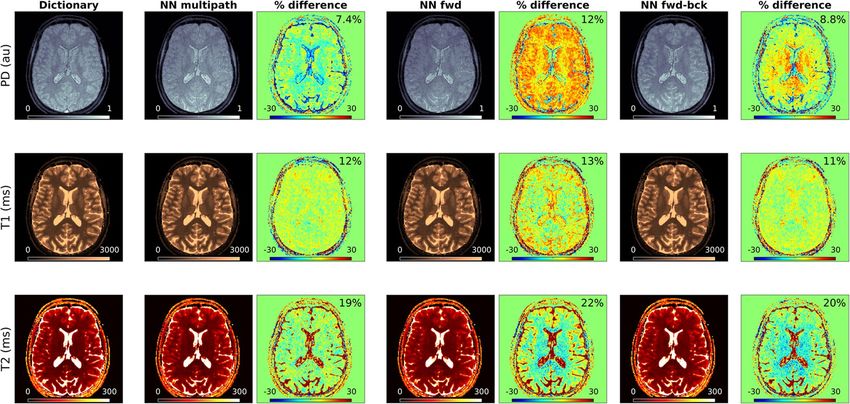
www.nature.com/scientificreports/
a b Iteration 1
Flip angle (degrees)
60 0.1 Iteration 2
Iteration 3
Signal (au)
40
20
0 0
0 200 400 600 800 0 2 4 6 8
Repetition index Time (s)
0.1
c T1 = 1000 ms, T2 = 80 ms
0.1
d T2 = 80 ms, T1 = 1000 ms
T1 = 800 ms T2 = 60 ms
T1 = 1200 ms T2 = 100 ms
Signal (au)
Signal (au)
0 0
0 2 4 6 8 0 2 4 6 8
Time (s) Time (s)
Figure 1. Excitation pattern. (a) The excitation pattern consists of a flip angle ramp to encode for T1 and
T2 followed by constant, small flip angles to allow for T1 recovery before the next inversion pulse. (b) Signal
evolutions reach a ‘steady’ transient-state after two iterations as magnetization before the inversion exhibits the
same initial conditions after the first iteration. (c, d) T1 and T2 encoding: T1 is encoded into the signal through
the inversion pulse prior to the flip angle train (c), whereas larger flip angle values produce spin echoes for T2
encoding (d).
Parameter 2D radial 2D spiral 3D radial 3D spiral 3D spiral (high-res)
Gradient amplitude (mT/m) 10 16 10 18 10
Slew rate (T/m/s) 70 80 70 60 90
Field of view (mm) 200 200 200 200 192
Matrix (mm) 200 200 200 200 200
Resolution (mm2/mm3) 1 1 1 1 0.96
Waveform duration (ms) 4.15 4.91 4.15 4.85 6.88
Acquired k-space samples per
496 920 496 876 1,348
interleave
Sampling time (ms) 1.98 3.68 1.98 3.50 5.39
TE (ms) 2.08 0.46 2.08 0.46 0.46
Number of in-plane interleaves 987 377 – 55 48
Number of spherical rotations – – – 880 576
Total interleaves 987 377 63,160 48,400 27,648
Acquired interleaves 880 880 49,280 49,280 28,224
Acquisition time @1.5 T 10.56 s 10.56 s 9:51 min 9:51 min –
Acquisition time @3 T 9.24 s 9.24 s 8:37 min 8:37 min 4:55 min
Table 1. Readout trajectories and experimental details.
when the in-plane rotations equaled the number of interleaves in the waveform design. Spherical rotations ena-
bled us to acquire data along all three spatial dimensions with fully sampled in-plane discs. Spherical rotations
were incremented with the golden angle from one repetition to the next, while in-plane rotations were incre-
mented linearly from one segment to the next.
Acquisition and reconstruction pipeline. All data were acquired following the excitation pattern shown in Fig. 1
with 880 repetitions per segment. Additionally, we accelerated the excitation pattern by reducing the total num-
ber of repetitions in Fig. 1a to 576, leading to a total acquisition time of 4:55 min. We acquired data with a
(192 mm)3 field of view and reconstructed onto a 2 003 matrix, resulting in 0.96 m m3 isotropic voxels. Table 1
summarizes the most important data acquisition parameters for all waveforms used in this work.
Acquired data were first anti-aliased with a k-space weighted view-sharing algorithm (Fig. 2) and recon-
structed following the pipeline presented in Fig. 3. The view-shared data are first projected into a lower dimen-
sional subspace with SVD compression to reduce the temporal signals to the first 10 SVD coefficients32 and
further reconstructed to obtain parametric maps and contrast-weighted images. In the following, we elaborate on
Scientific Reports | (2020) 10:13769 | https://doi.org/10.1038/s41598-020-70789-2 3
Vol.:(0123456789)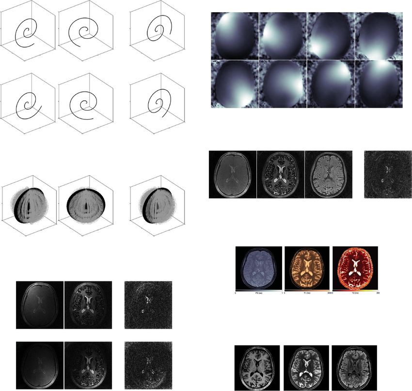
www.nature.com/scientificreports/
Figure 2. k-space weighted view-sharing with different acquisition trajectories. k-space weighted view-sharing
consists of sharing spatial acquisition data within neighboring temporal frames to increase the number of
samples per frame. This technique can be applied to all non-Cartesian trajectories, i.e. 2D radial (a), 2D spiral
(b), 3D radial (c) and 3D spiral (d) readouts.
steps b (k-space weighted view-sharing), f (parameter inference with artificial neural networks), and g (contrast-
weighted image synthesis) of the acquisition and reconstruction pipeline (see Fig. 3).
Anti‑aliasing via k‑space weighted view‑sharing. To anti-alias prior to parameter inference, we used k-space
weighted view-sharing. This algorithm builds upon the concept of k-space weighted image contrast33 and has
been used previously in the context of quantitative multiparametric mapping for C artesian19 and 2D radial
20
imaging . This method takes advantage of the fact that image contrast lies primarily within the central region of
k-space, which is also oversampled. This enables the application of different filters in distinct k-space regions in
order to enhance or reduce the contribution of each acquired view at each k-space location.
The method can be efficiently formulated as a linear weighted matrix multiplication in k-space, where the
multiplication weights control the amount of sharing per view and k-space location. In our implementation, and
different to Cruz et al.20, we set the weights as a function of the sampling density in all three spatial dimensions
instead of the distance to the center of k-space, enabling us to compare readouts with distinct density patterns
(i.e. spirals and radials). A further explanation of our view-sharing algorithms can also be seen in Supplementary
Fig. 1.
Scientific Reports | (2020) 10:13769 | https://doi.org/10.1038/s41598-020-70789-2 4
Vol:.(1234567890)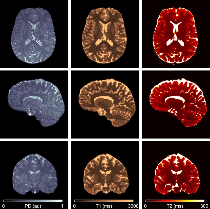
www.nature.com/scientificreports/
Figure 3. Data acquisition and reconstruction pipeline. (a) Undersampled data are acquired throughout
different repetitions with unique contrasts and distinct segments with equivalent contrasts. (b) k-space weighted
view-sharing increases the total amount of acquired samples per repetition. (c) Data are dimensionality reduced
and reconstructed to produce one image per coil and subspace coefficient. (d, e) Sensitivity maps are computed
and data from different receiver coils are combined. (f) Parameter inference produces quantitative maps as an
output. (g) The maps can subsequently be used to synthesize contrasts for qualitative imaging.
In order to assess the contribution of view-sharing, we performed the following numerical experiment.
We simulated the acquisition of time-domain data of a single representative white matter voxel (T1 = 600 ms,
T2 = 70 ms) using all of the introduced undersampled trajectories. The data were then reconstructed with steps
a-c of the pipeline to obtain a PSF in image space for each temporal coefficient. Data from the central 8 voxels
were Fourier interpolated onto a 200-voxel grid for better visualization of the sidelobes. We reconstructed the
data with both naïve zero-filling and view-sharing reconstruction. In addition, data corresponding to a fully
sampled experiment were generated as a reference. We compared the results in terms of the suppression of the
sidelobes and broadening of the PSF.
Parameter inference with artificial neural networks. Inspired by previous work17, we rely on a fully-connected
neural network for multi-parameter inference. By doing so, we embed the Bloch temporal dynamics by compact
Scientific Reports | (2020) 10:13769 | https://doi.org/10.1038/s41598-020-70789-2 5
Vol.:(0123456789)www.nature.com/scientificreports/
Figure 4. Neural network architectures for parameter inference. The neural networks receive the complex
signal in SVD subspace and infer the underlying tissue parameter vector θ based on different architectures. (a)
The multi-pathway implementation (NN multipath) is designed such that each path specializes on the estimation
of one parameter, parameter θi, i.e. T1, T2 or a PD related scaling factor. (b) The single pathway (NN fwd)
architecture has the total number of nodes as the NN multipath but directly infers the parameter vector from the
same hidden layers. (c) Parameters can also be derived from an autoencoder network (NN fwd-bck), where T1
and T2 are directly inferred from the latent space and relative PD is computed from the decoded output signal.
piecewise linear approximations rather than inefficient pointwise approximations used in the dictionary match-
ing. In this work, we introduced the estimation of PD by developing and evaluating three distinct neural network
architectures: a multi-pathway network with a single output parameter per pathway (NN multipath), a forward
network with three output parameters (NN fwd), and an encoder-decoder network with two parameters in the
encoded latent space and an output equivalent to the input (NN fwd-bck). This last alternative allows us to esti-
mate PD in an identical manner to dictionary matching techniques.
Neural network architectures. The proposed neural network architectures are illustrated in Fig. 4. All models
were designed to learn the non-linear relationship between the complex signal x as input, and the underlying
tissue parameters θ , where the input layer of each network receives the complex signal in SVD space x ∈ C10
instead of the full temporal signal evolution. This lower dimensional input enables the network to be easily
trained (e.g. using a CPU) and further avoids over-parametrization and the risk of overfitting. The input layer
is followed by a phase a lignment17,34 to work with real-valued instead of complex-valued measurements, and a
signal normalization layer.
Instead of a single-pathway architecture17,35–37, our proposed NN multipath architecture (Fig. 4a) splits param-
eter inference into individual pathways, wherein each specializes in the prediction of one parameter. Each branch
comprises 3 hidden layers with ReLU activations and 200, 100, and 1 node, respectively.
∼ ∼ ∼ The∼ final nodes of these
parametric pathways are then concatenated to form the parametric output θ = (θ 1 , θ 2 , θ 3 ) ∈ R3, representing
an estimate for T1 and T2, along with ∼ the norm of the simulated signals as a proxy for PD. From this scaling
factor, we can compute the relative PD ρ as
∼ �x�2
ρ= ∼ , (1)
θ3
where x 2 represents the 2-norm of the acquired signal x . The NN fwd architecture is a simplification of the
NN multipath with the same total number of nodes, wherein all output parameters are inferred directly from
the same hidden layers (Fig. 4b).
While both of these networks allow us to compute relative PD via Eq. 1, the mathematical formulation is not
identical to dictionary matching techniques. Thus, we created a third architecture, NN fwd-bck, by concatenat-
ing a two-path network with a single-path model with reversed hidden layers (Fig. 4c). This architecture can be
considered an∼autoencoder, as this model first infers parameters into a latent space and subsequently obtains an
output signal x equivalent to its input. In this model, the encoding portion is used to infer T1 and T2 while the
Scientific Reports | (2020) 10:13769 | https://doi.org/10.1038/s41598-020-70789-2 6
Vol:.(1234567890)www.nature.com/scientificreports/
Figure 5. Temporal data processing pipeline with neural network parameter inference. The letters follow the
same order as Fig. 3, where the neural network architecture corresponding to the multi-pathway network is
shown in (f). After dimensionality reduction via SVD subspace projection (c), gridding, FFT, coil estimation and
combination (c–e) are all linear operations that do not affect the input of the compressed signal into the neural
network. The output of the network is subsequently used to synthesize image contrasts (g).
∼
decoding
∼ portion acts as a Bloch simulator to create the output signal x . It is then possible to infer the relative
PD ρ in an identical way as is done with dictionary matching techniques
∼
∼ �x, x�
ρ= ∼ . (2)
� x �2
In all formulations, the inference of the relative PD within the neural network framework allowed us to use
it along other quantitative parameters to subsequently synthesize multiple clinical contrasts via the solutions
of the Bloch equations. Figure 5 illustrates the data processing pipeline from a temporal viewpoint, including
neural network parameter inference (Fig. 5f) and contrast synthesis (Fig. 5g).
Neural network training and validation. Based on Extended Phase G raphs38, we created a dataset of synthetic
signals of 52,670 samples for T1 = [10 ms, 5,000 ms] and T2 = [10 ms, 2,000 ms] to train our neural networks and
to obtain a dictionary matching reference. T1 values were simulated in steps of 1 ms from 10 to 2,000 ms and in
steps of 100 ms from 2,100 ms to 5,000 ms. T2 values were simulated in steps of 5 ms between 10 and 300 ms,
and in steps of 10 ms between 310 and 2,000 ms. In fact, we trained each neural network individually for each set
of acquisition parameters (2D and 3D spirals and radials). This was done because the 3D scheme varies slightly
from the 2D implementation, as the 3D acquisition requires a second iteration for the signal (Fig. 1b) and we
included the slice profile in the simulation39,40 for the 2D case. Also, we used a different TR for 1.5 T and 3 T
acquisitions.
For robust model training, we corrupted 80% of the generated samples with zero-mean independent Gauss-
ian noise and randomly varied SNR between 30 to 70 dB. We trained all networks on input batches of size 100,
using gradient descent optimization with a learning rate of 0.005 and the loss function J defined as the mean
absolute percentage error
∼ n
N
1
θ ′ n − θ ′
J=
θ ′ n
, (3)
N
n=1
∼n
where n ranges over all samples in the training set, θ ′ is the multiparametric output vector, and θ ′ n the corre-
sponding ground truth for sample n. The dropout rate was set to 0.9 and the model was trained for 500 epochs,
keeping the model that achieved the best performance on the validation data, i.e. the remaining 20% of the
samples. The stopping criterion was found empirically from previous experiments as the validation loss was
stable at this point. All networks were developed using TensorFlow.
To evaluate network inference we compared the reconstruction quality and computation times with exhaus-
tive grid search (dictionary matching) and fast group m atching41, which was implemented with 80 groups and
32
SVD compression . Image reconstruction and parameter inference were performed on an Intel Xeon processor
Scientific Reports | (2020) 10:13769 | https://doi.org/10.1038/s41598-020-70789-2 7
Vol.:(0123456789)www.nature.com/scientificreports/
E5-2,600 v4 (48 CPU cores) equipped with a NVIDIA Tesla K80 GPU (using the gpuNUFFT package for
regridding42).
Contrast‑weighted image synthesis. To allow radiological assessments, we used the parameters
inferred from the neural network to synthesize three different clinical contrasts: (1) a spoiled gradient recalled
echo (SPGR) with TR = 5.83 ms, FA = 13°, (2) a fast spin echo (FSE) using TE = 100 ms; and (3) a fluid attenuated
inversion recovery (FLAIR) based TE = 84.812 ms, and TI = 2,500 ms. In SPGR, contrast is dominated exclu-
sively by TR and T1
sinα(1 − e−TR/T1 )
SGRE = ρ TR
, (4)
(1 − cosαe− T1 )
while FSE contrast is driven by TE and T2
SFSE = ρe−TE/T2 , (5)
and FLAIR contrast is determined by both T1 and T2:
SFLAIR = ρe−TE/T2 (1 − 2e−TI/T1 ). (6)
To evaluate the effectiveness of our synthetic images, we compared them with standard acquisitions with
matching imaging parameters.
In vitro validation. We acquired the same tubes of the Eurospin TO5 phantom43 on a 1.5 T (GE HDxt) and
3 T (GE 750w) using all waveforms. To evaluate the impact of view-sharing, we reconstructed the data using
either only SVD p rojection32 or k-space weighted view-sharing followed by SVD projection (KW-SVD), and
subsequently inferred the parameters via each trained neural network. To assess accuracy and precision of the
predictions, bias and standard deviation of T1/T2 values were calculated for each vial. In addition, concordance
correlation coefficients44 (CCC) and normalized root mean square errors (NRMSE) were calculated at both
field strengths for each trajectory and for both SVD and KW-SVD reconstructions. NRMSE was normalized
with respect to the average of the nominal values of the vials. As a reference, we used the gold standard values
reported in the phantom’s manual together with our own measurements using FISP-MRF from Jiang et al.45, as
it has been previously validated for repeatability and reproducibility46,47.
In vivo validation. The study was conducted according to the principles of the Helsinki Declaration. All
subjects gave their informed consent to the enrollment in the study protocol GR-2016-02361693, approved by
the local competent ethical committee, the Comitato Etico Pediatrico Regionale (CEPR) of Regione Toscana,
Italy. We used the same protocol to acquire volunteer data at 1.5 T and 3 T, reconstructing the data with and
without view-sharing and estimating parameters with dictionary matching and neural network inference. Rep-
resentative ROIs were manually drawn in white matter and gray matter to quantitatively compare our results to
previous literature reports.
Results
Impact of readout trajectories and view‑sharing reconstruction. Figure 6 shows the results of the
PSF analysis. Our PSF analysis shows that all undersampled readouts approximate the fully-sampled PSF for
the first SVD coefficient, whereas view-sharing significantly improves the PSF with respect to zero-filling in
other lower energy coefficients, such as the ninth, where the sidelobes of the PSF were reduced by an order of
magnitude.
Figure 7 showcases the results for 1.5 T, where we focus on contrasting the different readout trajectories
and the impact of SVD compression alone versus view-sharing followed by SVD compression (KW-SVD). The
benefits of view-sharing can be most clearly visualized in the T1 maps for 3D radial and 3D spiral trajectories,
where higher spatial consistency can be achieved without negatively impacting sharpness or quantification
accuracy. However, trajectories with high undersampling factors, such 3D radial, still present clearly visible
artifacts that translate into blurred T2 maps. Overall, 3D spirals achieved the most efficient sampling coverage
and in combination with view-sharing, could best approximate the fully sampled PSF throughout different
spatiotemporal coordinates.
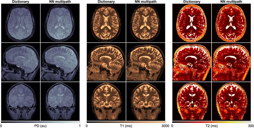
Neural network inference. Figure 8 compares dictionary matching against multi-path neural network
inference for the in vitro validation using the 3D spiral acquisition at 3 T. Here, we observe a high degree of cor-
relation between dictionary matching and network inference, where 95% confidence intervals lie within 6.58%
difference of each other. We further validated the neural network inference results against gold standard phan-
tom references for both the standard case and the accelerated, high-resolution version. We display these results
in Supplementary Figs. 2–4 and Tables 2 and 3, and elaborate on them in the next section.
Trained once, neural networks allow us to infer high resolution maps with quantification accuracy and image
quality compared to dictionary matching results as seen in Fig. 9, which presents representative 3 T results
based on the 3D spiral acquisition scheme. The high degree of agreement between neural network inference and
dictionary matching is confirmed by Fig. 10, where we depict a voxel-wise comparison based on the percentage
difference between neural network prediction and dictionary matching results.
Scientific Reports | (2020) 10:13769 | https://doi.org/10.1038/s41598-020-70789-2 8
Vol:.(1234567890)www.nature.com/scientificreports/
1 4 9
1
a
2D radial
0.5
0
1
Relative signal intensity (au)
b
2D spiral
0.5
0
1
c
3D radial
0.5
0
1
d
3D spiral
0.5
0
-4 -2 0 2 4 -4 -2 0 2 4 -4 -2 0 2 4
X-axis (pixel) X-axis (pixel) X-axis (pixel)
Reference Zero-filling View-sharing
Figure 6. Point spread function analysis. The PSF analysis evidences that view-sharing reconstruction is
beneficial when considering lower energy SVD coefficients. Without view-sharing, the PSF will have increased
sidelobes for all trajectories, most notably in 2D and 3D radials. φn represents the n-th SVD coefficient.
Figure 7. Readout trajectories and reconstruction comparison. A comparison of the different readout
trajectories evidences that, while all could be used multiparametric mapping, 3D radials suffer from larger
undersampling artifacts. Moreover, view-sharing improves spatial consistency without impacting parameter
quantification.
Scientific Reports | (2020) 10:13769 | https://doi.org/10.1038/s41598-020-70789-2 9
Vol.:(0123456789)www.nature.com/scientificreports/
20 20
a b
Percentage difference
Percentage difference
10 10
0 0
-10 -10
-20 -20
0 400 800 1200 1600 0 50 100 150 200 250
T1 (ms) T2 (ms)
Figure 8. Multipath neural network-based parameter inference—in vitro validation. 95% confidence intervals
in percentage differences to the dictionary are − 4.45–6.00% for T1 and − 3.97–6.58% for T2.
CCC SVD CCC KW-SVD NRMSE SVD (%) NRMSE KW-SVD (%)
T1 1.5 T
2D radial 0.99 0.98 10.26 11.0
2D spiral 0.99 0.99 8.4 8.5
3D radial 0.99 0.99 9.4 6.6
3D spiral 0.99 0.99 5.6 4.2
T2 1.5 T
2D radial 0.99 0.99 14.7 11.1
2D spiral 0.99 0.99 11.6 9.0
3D radial 0.99 0.99 15.3 10.5
3D spiral 0.98 0.98 7.0 4.9
T1 3 T
2D radial 0.99 0.98 8.3 10.1
2D spiral 0.99 0.98 6.2 10.4
3D radial 0.99 0.99 9.5 8.7
3D spiral 0.99 0.99 7.7 6.4
T2 3 T
2D radial 0.99 0.99 13.5 10.1
2D spiral 0.92 0.94 13.5 12.7
3D radial 0.99 0.99 13.7 11.0
3D spiral 0.97 0.98 9.6 7.6
Table 2. Phantom validation results for parameter inference using the NN multipath architecture. NRMSE
normalization were calculated with respect to the average nominal value of the vials.
T1 WM (ms) T2 WM (ms) T1 GM (ms) T2 GM (ms)
1.5 T
Previous reports48–50 788–898 63–80 1,269–1,393 78–117
SVD 600 ± 221 53 ± 20 1,189 ± 239 92 ± 32
2D radial
KW-SVD 731 ± 67 64 ± 8 1,046 ± 90 89 ± 14
SVD 677 ± 96 56 ± 12 1,041 ± 243 92 ± 30
2D spiral
KW-SVD 774 ± 49 64 ± 7 1,004 ± 104 87 ± 15
SVD 699 ± 225 64 ± 24 1,337 ± 422 132 ± 109
3D radial
KW-SVD 688 ± 117 63 ± 13 1,381 ± 304 112 ± 17
SVD 647 ± 60 65 ± 23 1,189 ± 119 101 ± 23
3D spiral
KW-SVD 630 ± 54 65 ± 7 1,192 ± 90 100 ± 14
Table 3. In vivo results using the NN multipath architecture. Results for representative ROIs within white
matter (WM) and gray matter (GM).
Scientific Reports | (2020) 10:13769 | https://doi.org/10.1038/s41598-020-70789-2 10
Vol:.(1234567890)www.nature.com/scientificreports/
Figure 9. Parameter inference via multipath neural network inference and dictionary matching. Inferring
parameter maps with a trained neural network and a high-resolution dictionary produces comparable
results—with the key difference that the network is not limited by dictionary size or its discretization grid, and
outperforms exhaustive grid search in terms of required memory and computation times.
Figure 10. Neural network-based parameter inference—in vivo validation. All neural network implementations
provide parametric estimates that are largely consistent with dictionary matching results. For all parameters,
the neural network architectures with separate pathways, i.e. NN multipath and NN fwd-bck, resulted in closer
estimates with respect to the dictionary than NN fwd, which is based on a single-pathway scheme.
Here, we specifically observe that PD estimates obtained with direct inference with the three-pathway network
NN multipath [via Eq. (1)] and with the autoencoder network NN fwd-bck [via Eq. (2)] are more consistent with
dictionary matching than the results of the single pathway network NN fwd. For the latter we visually observe
diminished tissue contrast in PD and higher percentage differences also for T1 and T2. We attribute these dif-
ferences to the simplicity of the NN fwd architecture, evidencing how naïve single-path architecture with shared
weights can result in declined performance for a subset of the output parameters. A multi-path architecture on
the other hand gives more flexibility to learn the physical relationship between the input signal and the individual
Scientific Reports | (2020) 10:13769 | https://doi.org/10.1038/s41598-020-70789-2 11
Vol.:(0123456789)www.nature.com/scientificreports/
Figure 11. Contrast-synthesis. The inclusion of PD to the inferred parameters enables high-quality contrast-
synthesis.
parameter. That is, the separate pathways of NN multipath and NN fwd-bck ensure that features that are essential
for the recovery of the individual parameters are retained, and not suppressed by other features which is a risk
a single-path schemes with shared weights. Thus, the NN multipath and NN fwd-bck produce higher fidelity
results as compared to a dictionary, and their modular architecture potentially enables the inclusion of additional
parameters beyond the ones considered in this study.
With the estimation of PD as an integral part of the neural network inference, it is now possible to produce
synthetic images from the inferred parameters showing typical contrasts used during radiological evaluations.
Figure 11 compares three typical contrasts—GRE, FSE, and FLAIR—obtained with our proposed technique
against standard clinical protocols. Moreover, Supplementary Fig. 5 displays a visualization of each of these
synthetic contrasts along the axial, sagittal, and coronal planes.
Quantification accuracy and precision. T1 and T2 quantification results with neural network inference
as compared to the gold standard reference are summarized in Supplementary Figs. 2–4 alongside Tables 2 and
3. Results for both 1.5 T and 3 T show that acquisitions using all tested readout trajectories are comparable to
the reference and could be used for multiparametric mapping within clinical settings: maximum quantification
bias for T1/T2 was less than 9/13% at 1.5 T and less than 9/15% at 3 T (Supplementary Fig. 3), while CCC were
higher than 0.98 for both T1 and T2 at 1.5 T, 0.92 for T2 quantification with the 2D spiral readout at 3 T, and
above 0.97 for all other cases (see Table 3).
While all the trajectories achieved a similar accuracy, 3D spiral trajectories showed substantially reduced
undersampling artifacts, resulting in a diminished standard deviation of the measurements (3–15% for T1, 4–11%
for T2 at 1.5 T; 3–14% for T1, 4–10% for T2 at 3 T). Conversely, quantification errors due to aliasing errors for
highly undersampled trajectories (such as 3D radial) were still present, leading to high standard deviations
(6–22% for T1, 11–27% for T2 at 1.5 T; 5–18% for T1, 10–29% for T2 at 3 T), as shown in Supplementary Fig. 3.
All trajectories (especially 3D trajectories) benefitted from the KW view-sharing processing, resulting in a
substantial reduction of aliasing artifacts: at 1.5 T, standard deviation contracted from 3–26 to 3–16% for T1 and
from 4–27 to 3–18% for T2, while at 3 T it diminished from 3–19 to 2–13% for T1 and from 4–29 to 3–20% for
T2 (Supplementary Fig. 3). In addition, KW view-sharing added only a minimal impact on the quantification
bias. The net effect was a reduction of the NRMSE of most of the measurements (see Table 2): at 1.5 T, NRMSE
decreased from 5.6–9.4% to 4.2–6.6% for T1 quantification of 3D readout trajectories, while it increased slightly
from 8.4–10.26 to 8.5–11% for 2D trajectories. For T2, it reduced from 7.0–15.3% to 4.9–11.1% for all trajec-
tories. At 3 T the reduction was again observable in 3D trajectories for T1 from 7.7–9.5 to 6.4–8.7% and in all
trajectories for T2, from 9.6–13.5 to 7.6–10.1%. We observed an increase in the NRMSE for T1 quantification
for 2D radial and 2D spiral measurements at 3 T from 6.2–8.3 to 10.1–10.4%.
In vivo experiments confirmed the results of the phantom experiment: T1/T2 values resulted in
600–774 ms/53–66 ms for white matter (compared to 788–898 ms/63–80 ms reported in literature48–50), and
1,004–1,381 ms/89–132 ms for gray matter (previous reports are 1,269–1,393 ms/78–117 ms). Reduction in
standard deviation due to KW view-sharing was comparable to the phantom experiment.
Acquisition and reconstruction efficiency. Table 1 reports acquisition times for all experiments,
whereas Table 4 compares reconstruction and inference times of dictionary matching, group matching, and
neural network parameter inference. For all cases, neural network inference significantly outperformed dic-
Scientific Reports | (2020) 10:13769 | https://doi.org/10.1038/s41598-020-70789-2 12
Vol:.(1234567890)www.nature.com/scientificreports/
Reconstruction time [s]
Zero-filling 2.2
CPU
View-sharing 5.8
2D
Zero-filling 0.6
GPU
View-sharing 4
Zero-filling 250
CPU
View-sharing 423
3D
Zero-filling 160
GPU
View-sharing 357
Inference time [s]
Dictionary 9.5
CPU Group matching 0.6
Neural network 0.1
2D
Dictionary 6.6
GPU Group matching 0.5
Neural network < 0.1
Dictionary 618
CPU Group matching 90
Neural network 10
3D
Dictionary 115
GPU Group matching 68
Neural network 10
Table 4. Reconstruction and inference times. Measurements were performed on an Intel Xeon processor
E5-2600 v4 (48 CPU cores) equipped with a NVIDIA Tesla K80 GPU. The inference times are compared
between exhaustive grid search (dictionary matching), fast group matching, and neural network. 2D results are
reported for a single slice of the spiral trajectory.
tionary matching and fast group matching techniques in terms of computation efficiency. In the accelerated
3D experiment, we achieved submillimeter resolution with an acquisition time of 4:55 min and reconstruction
and parameter inference times of 6:07 min using the proposed view-sharing technique and GPU gridding. The
results of this high-resolution and accelerated mapping experiment are displayed in Fig. 12. For a clearer visuali-
zation of the brain, we removed all non-brain tissue with the FSL brain extraction t ool51.
Discussion
In this work, we developed a quantitative parameter inference pipeline based non-iterative anti-aliasing, which
takes advantage of the computational efficiencies arising from subspace dimensionality reduction and neural
network parameter inference. We compared the performance of this pipeline on data obtained from different 2D
and 3D non-Cartesian trajectories. Our systematic comparisons confirmed that that spiral k-space trajectories
have higher sampling efficiency than radial. On the other hand, all readouts benefitted from k-space weighted
view-sharing.
All waveforms studied had a higher sampling density near the center of k-space, thus could accurately capture
contrast information while relying on view-sharing to recover the sparsely sampled outer portions of k-space.
Importantly, we showed that quantification values of T1 and T2 did not depend on the specific trajectory used
and agreed with the reference values from the Eurospin TO5 datasheet. On the other hand, slight T2 underesti-
mation was observed for all our measurements in vivo, when compared to literature value (steady-state or spin
echo method). We hypothesize this is due to effects not included in our inference model, such as unmodelled
k-space trajectory errors, diffusion or magnetization transfer effects. Further extension of the physical models
at the basis of our inference can establish the impact of these effects on accuracy and precision of the estimates.
A general limitation of performing inference on undersampled transient-state imaging is the presence of
errors due to aliasing, as a consequence of undersampling the k-space differently in each repetition. Artifacts
in image domain can be reduced by temporal compression, but temporal compression models usually do not
take k-space encoding into account, and specific anti-aliasing strategies have proven advantageous prior to
estimating the p arameters4,21,22,52. Amongst anti-aliasing methods, iterative approaches have limitations for full
three-dimensional non-Cartesian acquisitions, where 3D gridding and inverse gridding would be required at
each step, significantly increasing the computational burden associated with spatial decoding. We found that
local quantification errors due to aliasing can be reduced by a simple non-iterative anti-aliasing technique,
allowing clearer images for radiological evaluations. The concept used here for anti-aliasing is similar to key-
hole imaging20,33, and assumes that the image contrast is mainly stored in the center of k-space, while the image
details, which are mostly unchanged between frames, are in the edges of k-space. As in principle the effect of
such temporal filters on the final map accuracy is unknown, the impact of k-space weighted view-sharing on
the PSF was systematically evaluated in the SVD space, finding that it has very little impact on the blurring of
Scientific Reports | (2020) 10:13769 | https://doi.org/10.1038/s41598-020-70789-2 13
Vol.:(0123456789)www.nature.com/scientificreports/
Figure 12. Accelerated mapping. The method presented here achieves submillimeter isotropic resolution
multiparametric mapping in under 5 min with efficient reconstruction and neural network parameter inference
in under 7 min.
the images, but greatly reduces the local quantification errors due to aliasing. As all the operations are linear,
the process can be formulated as a series of simple operations, having a minor impact on reconstruction time.
We have demonstrated that anti-aliasing techniques used reduce artifacts on the final maps, while introduc-
ing only minimal apodization. However, our method still relies on assumptions on the k-space distribution of
contrast information, and highly undersampled acquisitions can still present visible artifacts, like for the case
of the 3D radial trajectory shown here. Methods tackling the optimization directly in the time domain, such as
MR-STAT5, have a superior artifact robustness because aliasing is not present in k-space. However, this comes
at the expense of computation time. Times reported for multi-slice MR-STAT have been of the order of several
hours on scientific computing clusters, which can limit clinical applicability. Future improvement of methods
including full spatial modelling such as MR-STAT could potentially improve on the efficiency of the estimates
presented here while keeping reasonable reconstruction times.
An important aspect of the method described here is the relatively high efficiency at encoding the tissue
properties into the transient-state signals. While here we have used a sequence with a simplified flip angle sched-
ule, various different strategies to optimize the acquisition are possible. For instance, it is possible to optimize
the Cramér-Rao Lower Bound of quantitative s equences9,13,14, recently demonstrated also in combination with
automatic differentiation algorithms, hence without approximations or an analytical formulation9. It is also
possible to use Bayesian design theory to define a set of optimal acquisition parameters for a particular range of
tissues of interest, maximizing both parameter encoding and experimental efficiency4. This approach could also
be used to systematically encode other MR-sensitive parameters such as diffusion or magnetization transfer into
transient-state signals. In alternative to transient-state acquisitions, pseudo-steady state methods (pSSFP)53,54
have demonstrated improved efficiency in terms of parameter encoding capabilities and the use of pSSFP may
further improve on the results shown here.
As an alternative to approaches using an exhaustive search over a grid representing a dictionary of simulated
evolution, performing the parameter estimation step via a neural network has several advantages28. First, storage
requirements for the network are much less restrictive than those of the dictionary. Second, parameter estima-
tions using neural networks are significantly faster than exhaustive searches over a predefined grid, especially
Scientific Reports | (2020) 10:13769 | https://doi.org/10.1038/s41598-020-70789-2 14
Vol:.(1234567890)www.nature.com/scientificreports/
Ma et al.10 Ma et al.12 Liao et al.7 Chen et al.36 Cao et al.11 Proposed
Trajectory Stack-of-spirals Music generated Stack-of-spirals Stack-of-spirals Spiral projections Spiral projections
1/0.8 mm Iso-
Resolution 1.2 × 1.2 × 3 mm3 2.3 Isotropic 1 mm Isotropic 1 mm Isotropic 0.96 Isotropic
tropic
300 × 300 × 144 300 × 300 × 300 260 × 260 × 192 260 × 260 × 180 240 × 240 × 240 192 × 192 × 192
Spatial coverage
mm3 mm3 mm3 mm3 mm3 mm3
Acquisition time 4.6 min 37 min 7.5 min 6.5–7.1 min 5/6 min < 5 min
Reconstruction
48 min N.A 20 h N.A 1.5-4 h < 7 min
time
Table 5. Previous reports of 3D MRF acquisitions as compared to our proposal.
if the model is estimated on a GPU. Third, under the assumption of local linearity of the Bloch manifold, the
network is not limited to a discretized set of parameter values. Our proposed network architectures were inspired
by recent work at the intersection of deep learning and quantitative mapping techniques, such as the MRF-Net
proposed in the study on geometry of deep learning for MRF17 and the deep reconstruction network (DRONE)35.
Both works demonstrated that dictionary matching for T1 and T2 mapping can be replaced with high accuracy
by a compact, fully-connected neural network trained on simulated signals. Moreover, whereas the DRONE
requires the full temporal signal and thus is computationally prohibitive for high-resolution 3D mapping, the
MRF-Net performs inference on dimensionality reduced signals. Our networks are motivated by these works,
whereas the proposed multi-pathway and autoencoding architectures alongside the integrated PD estimation
are a significant technical novelty with respect to previous implementations.
Only now, the neural network-based parameter inference can fully replace the dictionary matching framework
as all previous works lacked the inference of a PD estimate which is required for subsequent synthetic image
generation. Also, the proposed multi-pathway model design presents an opportunity for compact transfer-
learning. Previous works either focused on single-pathway implementations where all output parameters emerge
from the same fully-connected branch or trained individual networks for each parameter to be estimated37,55,56.
Here, we formulate the multivariate regression as a single joint optimization, but give the network more freedom
in finding the non-linear input–output mappings compared to single-pathway schemes, as each pathway can
specialize in the inference of one parameter. At the same time, we prevent overfitting of one specific task due to
the regularizing and balancing capacity of the joint loss. The increased flexibility provided by the multi-pathway
model could also facilitate an extension to additional parameters as MR sequences are continuously developed
to simultaneously encode for more information.
Other recent works rely on spatially constrained, convolutional neural networks, such as U-Net
architectures37,55, for parameter inference in high-resolution MRF experiments. Although these approaches
have shown to provide high quality parameter maps, they are based on the dictionary matching results for model
training, which cannot be considered a ground truth. In contrast to the recently proposed U-Net architectures,
we present a compact model that facilitates training and parameter inference even on CPUs. Our neural network
is trained on purely synthetic signal time-courses. Its performance is independent of and hence not bound by the
quality and accuracy of dictionary matching results. Once trained, the proposed model is then universally—in
terms of anatomical region and patient pathologies—applicable in a clinical setting. This might not be the case
for spatially constrained networks which have only seen e.g. healthy brain tissue during training.
The combination of simple and efficient anti-aliasing with a multi-pathway neural network parameter infer-
ence allowed us to reconstruct a full 3D volume with sub-millimeter resolution in under 7 min using a high-
performing server (see system details in Table 4). We consider this an important result, as current state-of-the-art
achieves comparable reconstructions within 4 h (see Table 5) and is limited by the dictionary discretization grid11.
Conclusion
Three-dimensional quantitative transient-state imaging provides an efficient framework for multiparametric
mapping, achieving high anatomical detail and quantification accuracy and precision. The novel introduction
of proton density in a compact, multi-path neural network, coupled with a computationally rapid anti-aliasing
technique, allowed us to acquire and reconstruct full volume, high-resolution isotropic data within clinically
acceptable times. Given this fast and comprehensive acquisition, the method proposed here can be used in chal-
lenging populations, including elderly patients and children. Our improved acquisition and reconstruction times
encourage further investigation towards clinical applications.
Data availability
The datasets generated during and/or analyzed during the current study are available from the corresponding
author on reasonable request.
Received: 8 November 2019; Accepted: 22 June 2020
Scientific Reports | (2020) 10:13769 | https://doi.org/10.1038/s41598-020-70789-2 15
Vol.:(0123456789)www.nature.com/scientificreports/
References
1. Tofts, P. Quantitative MRI of the Brain: Measuring Changes Caused by Disease (Wiley, Hoboken, 2003).
2. Ma, D. et al. Magnetic resonance fingerprinting. Nature https://doi.org/10.1038/nature11971 (2013).
3. Warntjes, J. B. M., Dahlqvist Leinhard, O., West, J. & Lundberg, P. Rapid magnetic resonance quantification on the brain: optimiza-
tion for clinical usage. Magn. Reson. Med. 60, 320–329 (2008).
4. Gómez, P. A., Molina-Romero, M., Buonincontri, G., Menzel, M. I. & Menze, B. H. Designing contrasts for rapid, simultaneous
parameter quantification and flow visualization with quantitative transient-state imaging. Sci. Rep. 9, 8468 (2019).
5. Sbrizzi, A. et al. Fast quantitative MRI as a nonlinear tomography problem. Magn. Reson. Imaging 46, 56–63 (2018).
6. Hargreaves, B. A., Vasanawala, S. S., Pauly, J. M. & Nishimura, D. G. Characterization and reduction of the transient response in
steady-state MR imaging. Magn. Reson. Med. https://doi.org/10.1002/mrm.1170 (2001).
7. Liao, C. et al. 3D MR fingerprinting with accelerated stack-of-spirals and hybrid sliding-window and GRAPPA reconstruction.
Neuroimage 162, 13–22 (2017).
8. Jiang, Y. et al. MR fingerprinting using the quick echo splitting NMR imaging technique. Magn. Reson. Med. 77, 979–988 (2016).
9. Lee, P. K., Watkins, L. E., Anderson, T. I., Buonincontri, G. & Hargreaves, B. A. Flexible and efficient optimization of quantitative
sequences using automatic differentiation of Bloch simulations. Magn. Reson. Med. 82, 27832 (2019).
10. Ma, D. et al. Fast 3D magnetic resonance fingerprinting for a whole-brain coverage. Magn. Reson. Med. 79, 2190–2197 (2018).
11. Cao, X. et al. Fast 3D brain MR fingerprinting based on multi-axis spiral projection trajectory. Magn Reson Med 82, 289 (2019).
12. Ma, D. et al. Music-based magnetic resonance fingerprinting to improve patient comfort during MRI examinations. Magn. Reson.
Med. https://doi.org/10.1002/mrm.25818 (2016).
13. Assländer, J., Lattanzi, R., Sodickson, D. K. & Cloos, M. A. Relaxation in spherical coordinates: analysis and optimization of
pseudo-SSFP based MR-fingerprinting. arXiv eprint (2017).
14. Zhao, B. et al. Optimal experiment design for magnetic resonance fingerprinting: cramér-rao bound meets spin dynamics. IEEE
Trans. Med. Imaging https://doi.org/10.1109/TMI.2018.2873704 (2019).
15. Gómez, P. A. et al. Accelerated parameter mapping with compressed sensing: an alternative to MR Fingerprinting. Proc. Int. Soc.
Mag. Reson. Med. (2017).
16. Sbrizzi, A., Bruijnen, T., Van Der Heide, O., Luijten, P. & Van Den Berg, C. A. T. Dictionary-free MR Fingerprinting reconstruction
of balanced-GRE sequences. arXiv eprint (2017).
17. Golbabaee, M. et al. Geometry of Deep Learning for Magnetic Resonance Fingerprinting, in ICASSP 2019—2019 IEEE Interna‑
tional Conference on Acoustics, Speech and Signal Processing (ICASSP) 7825–7829 (IEEE, 2019). https://doi.org/10.1109/ICASS
P.2019.8683549
18. Cao, X. et al. Robust sliding-window reconstruction for accelerating the acquisition of MR fingerprinting. Magn. Reson. Med. 78,
1579–1588 (2017).
19. Buonincontri, G. & Sawiak, S. Three-dimensional MR fingerprinting with simultaneous B1 estimation. Magn. Reson. Med. 00, 1–9
(2015).
20. Cruz, G. et al. Accelerated magnetic resonance fingerprinting using soft-weighted key-hole (MRF-SOHO). PLoS ONE 13, e0201808
(2018).
21. Davies, M., Puy, G., Vandergheynst, P. & Wiaux, Y. A compressed sensing framework for magnetic resonance fingerprinting. SIAM
J. Imaging Sci. 7, 2623–2656 (2014).
22. Gómez, P. A. et al. Learning a spatiotemporal dictionary for magnetic resonance fingerprinting with compressed sensing. MICCAI
Patch-MI Work 9467, 112–119 (2015).
23. Pierre, E. Y., Ma, D., Chen, Y., Badve, C. & Griswold, M. A. Multiscale reconstruction for MR fingerprinting. Magn. Reson. Med.
https://doi.org/10.1002/mrm.25776 (2016).
24. Zhao, B. et al. Improved magnetic resonance fingerprinting reconstruction with low-rank and subspace modeling. Magn. Reson.
Med. https://doi.org/10.1002/mrm.26701 (2018).
25. Assländer, J. et al. Low rank alternating direction method of multipliers reconstruction for MR fingerprinting. Magn. Reson. Med.
79, 83–96 (2018).
26. Gómez, P. A. et al. 3D magnetic resonance fingerprinting with a clustered spatiotemporal dictionary. Proc. Int. Soc. Magn. Reson.
Med. (2016).
27. Gómez, P. A. et al. Simultaneous parameter mapping, modality synthesis, and anatomical labeling of the brain with MR finger-
printing. MICCAI Int. Conf. Med. Image Comput. Comput. Interv. LNCS 9902, 579–586 (2016).
28. Cohen, O., Zhu, B. & Rosen, M. Deep learning for fast MR fingerprinting reconstruction. Proc. Int. Soc. Magn. Reson. Med. (2017).
29. Pirkl, C. M. et al. Deep learning-based parameter mapping for joint relaxation and diffusion tensor MR Fingerprinting. Proc. Mach
Learn. Res. (2020).
30. Balsiger, F. et al. Magnetic resonance fingerprinting reconstruction via spatiotemporal convolutional neural networks. Mach. Learn.
Med. Image Reconstr. 11074, 39–46 (2018).
31. Hargreaves, B. A., Nishimura, D. G. & Conolly, S. M. Time-optimal multidimensional gradient waveform design for rapid imaging.
Magn. Reson. Med. 51, 81–92 (2004).
32. McGivney, D. F. et al. SVD compression for magnetic resonance fingerprinting in the time domain. IEEE Trans. Med. Imaging
https://doi.org/10.1109/TMI.2014.2337321 (2014).
33. Song, H. K. & Dougherty, L. k-space weighted image contrast (KWIC) for contrast manipulation in projection reconstruction
MRI. Magn. Reson. Med. 44, 825–832 (2000).
34. Golbabaee, M., Chen, Z., Wiaux, Y. & Davies, M. E. CoverBLIP: accelerated and scalable iterative matched-filtering for magnetic
resonance fingerprint reconstruction. Inverse Probl. 36, 015003 (2019).
35. Cohen, O., Zhu, B. & Rosen, M. S. MR fingerprinting deep reconstruction network (DRONE). Magn. Reson. Med. https://doi.
org/10.1002/mrm.27198(2018).
36. Chen, Y. et al. High-resolution 3D MR fingerprinting using parallel imaging and deep learning. Neuroimage https://doi.
org/10.1016/j.neuroimage.2019.116329 (2020).
37. Fang, Z. et al. Deep learning for fast and spatially constrained tissue quantification from highly accelerated data in magnetic
resonance fingerprinting. IEEE Trans. Med. Imaging https://doi.org/10.1109/TMI.2019.2899328 (2019).
38. Weigel, M. Extended phase graphs: dephasing, RF pulses, and echoes: pure and simple. J. Magn. Reson. Imaging https://doi.
org/10.1002/jmri.24619(2014).
39. Buonincontri, G. & Sawiak, S. J. MR fingerprinting with simultaneous B1 estimation. Magn. Reson. Med. 76, 1127–1135 (2016).
40. Ma, D. et al. Slice profile and B1 corrections in 2D magnetic resonance fingerprinting. Magn. Reson. Med. 78, 1781–1789 (2017).
41. Cauley, S. F. et al. Fast group matching for MR fingerprinting reconstruction. Magn. Reson. Med. https: //doi.org/10.1002/mrm.25439
(2014).
42. Knoll, F., Schwarzl, A., Diwoky, C. gpuNUFFT: An open-source GPU library for 3D gridding with direct matlab interface. Proc.
Int. Soc. Magn. Reson. Med. (2014).
43. Lerski, R. A. & de Certaines, J. D. Performance assessment and quality control in MRI by Eurospin test objects and protocols.
Magn. Reson. Imaging 11, 817–833 (1993).
44. Lin, L.I.-K. A concordance correlation coefficient to evaluate reproducibility. Biometrics 45, 255 (1989).
Scientific Reports | (2020) 10:13769 | https://doi.org/10.1038/s41598-020-70789-2 16
Vol:.(1234567890)You can also read