Retrieving horizontally resolved wind fields using multi-static meteor radar observations
←
→
Page content transcription
If your browser does not render page correctly, please read the page content below
Atmos. Meas. Tech., 11, 4891–4907, 2018
https://doi.org/10.5194/amt-11-4891-2018
© Author(s) 2018. This work is distributed under
the Creative Commons Attribution 4.0 License.

Retrieving horizontally resolved wind fields using multi-static
meteor radar observations
Gunter Stober1 , Jorge L. Chau1 , Juha Vierinen2 , Christoph Jacobi3 , and Sven Wilhelm1
1 Leibniz-Institute  of Atmospheric Physics, Schlossstr. 6, 18225 Kühlungsborn, Germany
2 Department    of Physics and Technology, The Arctic University of Norway, Tromsø, Norway
3 Institute for Meteorology, Universität Leipzig, Stephanstr. 3, 04103 Leipzig, Germany

Correspondence: Gunter Stober (stober@iap-kborn.de)

Received: 26 March 2018 – Discussion started: 3 April 2018
Revised: 17 July 2018 – Accepted: 10 August 2018 – Published: 27 August 2018

Abstract. Recently, the MMARIA (Multi-static, Multi-               horizontally resolved wind fields at mesospheric altitudes,
frequency Agile Radar for Investigations of the Atmosphere)        needed to access small scale variations associated to grav-
concept of a multi-static VHF meteor radar network to derive       ity waves (GWs). GWs are considered to be a major driver
horizontally resolved wind fields in the mesosphere–lower          of MLT dynamics as they carry energy and momentum from
thermosphere was introduced. Here we present preliminary           other (mainly lower) atmospheric layers into the mesosphere
results of the MMARIA network above Eastern Germany                (Fritts and Alexander, 2003; Becker, 2012).
using two transmitters located at Juliusruh and Collm, and            Over the past few decades specular meteor radars (SMRs)
five receiving links: two monostatic and three multi-static.       have become a reliable and widespread tool to investigate
The observations are complemented during a one-week cam-           mesospheric mean winds (e.g., Elford, 1959; Roper, 1975;
paign, with a couple of addition continuous-wave coded             Nakamura et al., 1991; Hocking et al., 2001; Hall et al., 2005;
transmitters, making a total of seven multi-static links. In or-   Jacobi et al., 2009; Stober et al., 2017; McCormack et al.,
der to access the kinematic properties of non-homogenous           2017; Wilhelm et al., 2017). These systems are also capable
wind fields, we developed a wind retrieval algorithm that ap-      of providing valuable information about gravity waves and
plies regularization to determine the non-linear wind field in     tides (Fritts et al., 2010a; Jacobi, 2011) as well as to estimate
the altitude range of 82–98 km. The potential of such ob-          the gravity wave momentum flux (e.g., Hocking, 2005; Fritts
servations and the new retrieval to investigate gravity waves      et al., 2010b; de Wit et al., 2014; Placke et al., 2015). In par-
with horizontal scales between 50–200 km is presented and          ticular, Fritts et al. (2012) pointed out that the quality of the
discussed. In particular, it is demonstrated that horizonal        gravity wave momentum flux strongly depends on the num-
wavelength spectra of gravity waves can be obtained from           ber of meteor detections per time interval and the diameter
the new data set.                                                  of the observation volume.
                                                                      The spatial and temporal intermittency of GWs are hardly
                                                                   accessible from point measurements. Airglow imagers (e.g.,
                                                                   Hecht et al., 2000, 2007) or the Advanced Mesospheric Tem-
1   Introduction                                                   perature Mapper (Taylor et al., 2009; Pautet et al., 2014) are
                                                                   able to observe small scale GWs as intensity or temperature
The upper mesosphere–lower thermosphere (MLT) is a                 fluctuations. However, due to the often missing background
highly dynamic region dominated by a variety of waves              wind information, the intrinsic GW properties can not be in-
(gravity waves, tides, planetary waves) covering different         ferred. Smith et al. (2017) combined the 2-D airglow infor-
spatial and temporal scales. To characterize this variability,     mation with MR wind measurements to investigate a bore
it is desirable to develop remote sensing techniques to re-        event across Europe and derived the intrinsic properties of
trieve horizontally resolved structures from continuous ob-        the GW. At present there are only a few attempts to measure
servations. A particular challenge is the determination of

Published by Copernicus Publications on behalf of the European Geosciences Union.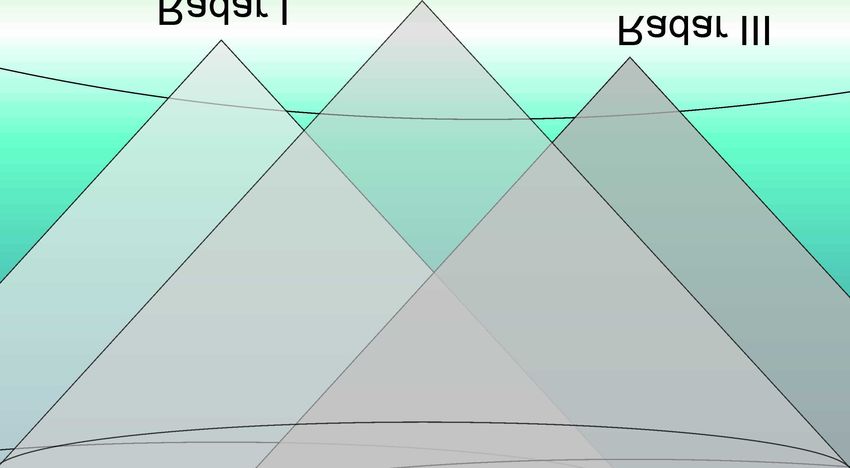
4892                                                                                              G. Stober et al.: MMARIA winds

                                                                       pendix contains all equations required for the WGS84 coor-
                                                                       dinate transformations.
                               M

                                                                       2   Wind analysis of mean meteor radar winds

                                                                       Meteors entering the Earth’s atmosphere form an ambipo-
                                                                       lar plasma trail, if they are fast and heavy enough. The trail
                                                                       is drifted by the ambient neutral winds at the altitude of its
                                                                       deposition. Combining the radial Doppler measurement with
                                                                       radar interferometry (Jones et al., 1998) permits the measure-
                                                                       ment of the radial velocity, range, and angle of arrival (here in
                                                                       mathematical convention as φ counterclockwise from East, θ
                                                                       off-zenith). Due to the huge number of meteor detections in
                                                                       the course of a day it is possible to determine the prevailing
Figure 1. Schematic of a multi-static meteor radar network. The        wind speeds by binning the observed meteors in space (verti-
grey shaded areas stand for the typical field of views for each sys-   cal) and time applying a so called all-sky fit (Hocking et al.,
tems. Within the network all system should at least overlap to one     2001; Holdsworth et al., 2004) over typically 1 h in time and
of the other network members.                                          a few kilometers in height.
                                                                          To increase the robustness of the standard wind fit estima-
                                                                       tion, e.g., better temporal resolution and altitude coverage, it
                                                                       is possible to use regularization by adding constraints based
horizontally resolved wind structures on comparable scales             on a priori information. Recently, we have implemented a
to airglow imagers by radars (Stober et al., 2013, 2018).              routine to derive mesospheric winds using full non-linear
   Recently, Stober and Chau (2015) introduced the                     error propagation, an additional weighting to account for
MMARIA (Multi-static Multi-frequency Agile Radar for In-               sampling effects, and a smoothness regularization. The er-
vestigation of the Atmosphere) concept to observe horizon-             ror propagation is straightforward as most of the available
tally resolved wind fields combining monostatic and multi-             systems provide errors for the radial velocity measurements.
static SMR observations. The MMARIA concept allows to                  The angular uncertainties are estimated to be in the order of
increase the number of detected meteors per transmitter,               2◦ (Jones et al., 1998). Further, the errors of the 3-D wind
an extended altitude coverage, and more even spatial sam-              components are estimated from the covariance matrix and
pling within the field of view, when compared to traditional           updated with each iteration. The sampling effects are mainly
monostatic SMRs. They demonstrated the potential to access             caused by meteors occurring randomly in space and time,
the kinematic properties of non-homogenous wind fields ap-             but we often analyze the winds on a fixed grid in time and
plying volume velocity processing (VVP) (Waldteufel and                altitude. Therefore, we apply an additional weighting, with a
Corbin, 1979) to the multi-static SMR observations, i.e., by           Gaussian kernel, to account for altitude and time differences
deriving the horizontal gradients of the horizontal wind com-          between the actual occurrence of a meteor and the reference
ponents, in addition to their mean values. The multi-static            time and altitude. The half width of the Gaussian kernel is
observation geometry allows the observation of almost the              given by the width of the altitude (dh) and time bins (dt).
same measurement volumes from different angles. Thus, it               The Gaussian weighting due to the randomness of the me-
is possible to access the first order inhomogeneities of the           teor occurrence is given by
mesoscale wind field, e.g., horizontal divergence, relative
                                                                                                        (tm − tref )2

vorticity, stretching, and shearing deformation. Here we are           σtime = Atshear − Atshear exp −                   ,          (1)
going to extent the existing approach to the retrieval of ar-                                          (0.5 · dtave )2
bitrary wind fields using multi-static observations of meteor          and for the altitude
radar networks. Figure 1 presents a schematic of such an net-
work.                                                                                                 (altm − altref )2

   The paper is structured as follows. In Sect. 2 we present           σalt = Aashear − Aashear exp −                     .         (2)
                                                                                                           dh2ave
a summary of the normal meteor radar wind retrieval. This
method is going to be expanded in Sect. 3 to horizontally re-             The temporal and vertical total shear amplitude Atshear and
solved winds in a full Earth geometry. In Sect. 4 we perform           Aashear are estimated from our temporal and vertical regu-
an initial validation and consistency check. The potential use         larization gradients from all three wind components. Typical
of the new horizontally resolved wind retrieval is given in            values are 2 h for dtave for a 1 h temporal resolution with over
Sect. 5 presenting first horizontal wavelength spectra. Our            sampling and 1.5 km for dhave for a 2 km vertical altitude res-
main conclusions are presented in the last section. The ap-            olution. The shear terms σtime and σalt are added to our total

Atmos. Meas. Tech., 11, 4891–4907, 2018                                                  www.atmos-meas-tech.net/11/4891/2018/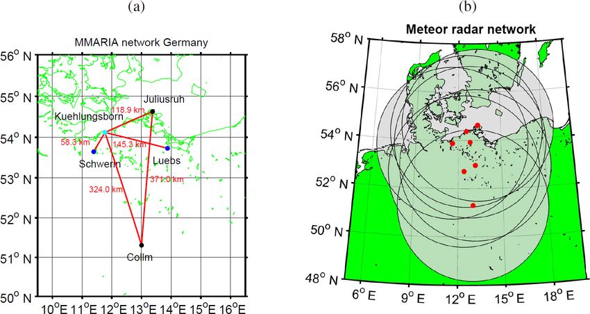
G. Stober et al.: MMARIA winds                                                                                                    4893

statistical error budget during each iteration together with all
other statistical uncertainties.
   The smoothness regularization scheme consists of the ver-
tical and temporal derivative for each wind component taken
as constant within each bin. The initial guess is given by
a standard least squares solution without any regularization
constraint, but already contains the Gaussian weighting with
σtime = 5 m s−1 and σalt = 5m s−1 . This solution is then used
for the next iteration and the new solution is constrained by
the previous one. Typically we need 3–5 iterations to achieve
convergence. Basically our wind estimates do not change
more than the statistical uncertainty, which is in the order of
1 − −6 m s−1 at altitudes between 82–95 km (typically 40–
250 meteors). At the edges of the meteor layer (below 82 km
or above 95 km) the error can reach up to 15–20 m s−1 as the
number of meteors (less than 15) used for each wind estimate         Figure 2. Illustration on how local coordinates (zonal, meridional)
drops significantly at these altitudes. More details about the       change with geographic position with respect to a radar location.
application of this algorithm can be found in Stober et al.
(2017). Further, in the manuscript we are referring to this
technique as “standard” method or “all-sky” fit.                     3     Wind analysis of arbitrary wind fields
   A bit more sophisticated than the “all-sky” fit is the so
called volume velocity processing (VVP) (Waldteufel and              3.1    Implementing the Earth geometry in the wind
Corbin, 1979). This method does no longer assume a ho-                      analysis
mogenous wind field within the observed volume. The wind
field is approximated by introducing gradient terms for the          A new aspect of the MMARIA concept is the necessity to
wind components.                                                     consider the geometry of the Earth. At present our domain
                                                                     area in Germany has a horizontal extension of approximately
         ∂u               ∂u                                         600 km × 600 km. These distances are too large to assume
u = u0 +    · (x − x0 ) +    · (y − y0 )                      (3)
         ∂x               ∂y                                         a plane geometry, which is very often the case for classi-
         ∂v               ∂v                                         cal monostatic MRs, where all observations are referred to
v = v0 +    · (x − x0 ) +    · (y − y0 )                      (4)
         ∂x               ∂y                                         the location of the radar itself. However, it is straightforward
w = w0                                                        (5)    to at least consider that the altitude or height above the sur-
                                                                     face needs to be corrected for the Earth curvature using a
   Here u0 , v0 , and w0 are the mean zonal, meridional and          mean Earth radius (RE = 6 378 137.0 m). Further, it is possi-
vertical wind components similar to the “all-sky” fit. The           ble to obtain a local elevation angle for each meteor, instead
partial derivatives are taken relative to a reference position       of the one observed relative to the receiver location. How-
(x0 , y0 ), which could be the position of a radar or an arbitrar-   ever, this simple correction turned out to still be insufficient
ily selected point somewhere between several radar systems.          for dealing with large domain areas. Therefore, we outline a
The mean winds as well as the gradient terms are similarly           more detailed procedure, taking into account the Earth shape
obtained as in the “all-Sky” fit using a regularization includ-      with the WGS84 geoid model (National Imagery and Map-
ing also the gradient terms. Due to the increased number of          ping Agency, 2000).
unknowns at least 10 meteors should be used for the fit. Chau           In the following we outline the procedure how to compute
et al. (2017) shows the equations in spherical coordinates.          new local coordinates (ENU: east–north–up) for each meteor
   Such an analysis does not only provide mean winds for             to reduce potential errors in the wind field estimation due to
each time and altitude bin, but also access higher order kine-       projection issues. Considering that the Earth is not a perfect
matic processes as horizontal divergence, relative vorticity         sphere, we have to deal with two different coordinates, the
as well as stretching and shearing deformation. In order to          geodetic coordinates (longitude and latitude) and the Earth-
unambiguously obtain the relative vorticity multi-static mea-        Centered, Earth-Fixed (ECEF) coordinates, also called geo-
surements are required (Stober and Chau, 2015; Chau et al.,          centric coordinates. The geodetic coordinates are determined
2017). Although the method already allows to access some             by the normal to the ellipsoid, whereas the ECEF coordinates
spatial information it is still not possible to retrieve the phase   are defined by the Earth center using a (X, Y , Z)-coordinate
speed of gravity waves within the volume or to obtain the            system. Thus, the geodetic and geocentric latitude can be dif-
spatial variability on much smaller scales than the observa-         ferent.
tion volume.                                                            We need to transform the observed meteor positions rela-
                                                                     tive to the radar into a local coordinate frame (ENU) by de-

www.atmos-meas-tech.net/11/4891/2018/                                                   Atmos. Meas. Tech., 11, 4891–4907, 2018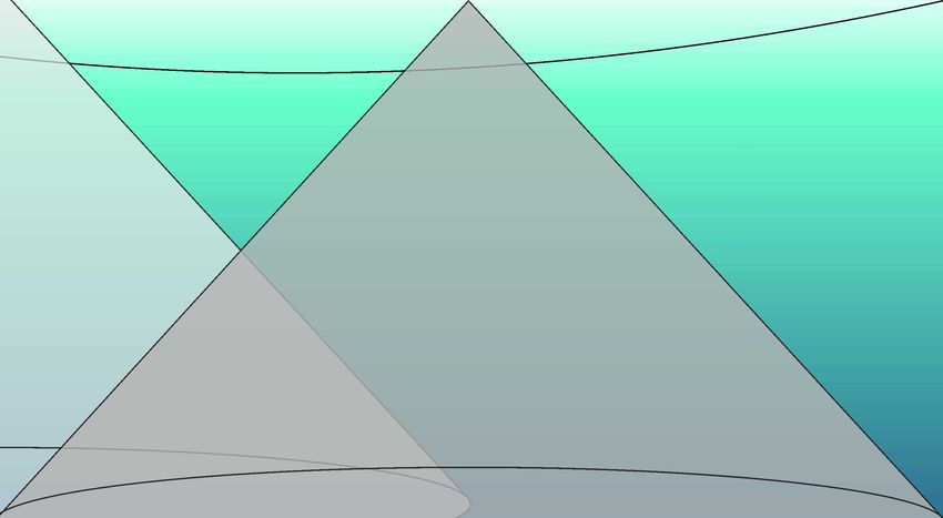
4894                                                                                         G. Stober et al.: MMARIA winds

termining the geodetic longitude, latitude and height of the                  g
meteor itself. The corresponding transformations are listed                                  H

in the appendix. The procedure contains four steps: firstly
the geodetic coordinates of the radar (longitude-φ,latitude-
λ, height-h) are converted into ECEF, which means we re-
ceive a vector x R = (XR , YR , ZR ), with respect to the Earth
center. From the interferometric solution we also know the
position vector x P = (x, y, z) with respect to the receiver lo-
cation for each meteor. This vector x P is then transformed              H
into ECEF coordinates and we obtain a vector pointing from
the Earth center towards the meteor position with coordi-
nates x M = (XM , YM , ZM ). Further, we convert the vector
x M given in ECEF coordinates back into a geodetic position
given by the latitude, longitude, and height above the Earth’s
surface for each meteor. Finally, we use the ECEF vector x M
and the geodetic reference to compute a local coordinate set       Figure 3. Schematic of 3-D gridding to compute horizontally re-
ENU at the position of the meteor itself. A detailed descrip-      solved wind fields including the Earth surface.
tion of all applied coordinate transformations is summarized
in the appendix.
   In summary we perform the following steps:                      standard analysis. In particular, altitudes where only a small
                                                                   number of meteors are used for the wind estimation proce-
 1. conversion of the geodetic coordinates of the radar            dure are more prone to this type of error. In particular, it ap-
    (φ, λ, h) → (XR , YR , ZR ) by using the transformation        pears to be very critical or in fact almost impossible to obtain
    geodetic to ECEF;                                              a reliable vertical wind velocity or momentum flux, if the full
 2. transformation of meteor coordinates into ECEF                 Earth geometry is not taken properly into account.
    (x, y, z) → (XM , YM , ZM ) by using the transformation
    of ENU to ECEF;                                                3.2   Retrieving arbitrary non-homogenous wind fields

 3. conversion of ECEF frame meteor position into geode-           The retrieval of arbitrary and non-homogenous wind fields is
    tic coordinates (XR , YR , ZR ) → (φ, λ, h) ECEF to            mathematically more demanding as the number of unknowns
    geodetic;                                                      exceeds the number of measurements, which does not al-
                                                                   low to directly solve the equations applying standard least
 4. determination of local ENU using the geodetic posi-
                                                                   squares or singular value decomposition algorithms. How-
    tion of each meteor in ECEF coordinates (φ, λ, h) →
                                                                   ever, it is possible to constrain the problem by additional as-
    (xM , yM , zM ).
                                                                   sumptions or a priori knowledge. Very often the smoothness
    Figure 2 shows an example of the difference between the        is used to regularize the problem so that it can be solved by
ENU coordinates (black cross) of the radar location and the        applying statistical inversion algorithms (Aster et al., 2013).
ENU coordinates (red cross) of a meteor observed at a hori-           At first we define a spatial grid and a domain area. In the
zontal distance of 300 km. The blue circle marks the 300 km        case of the German MMARIA network we use a 30 km ×
range around the radar, which is assumed to be located at          30 km grid spacing in zonal and meridional direction. The
Juliusruh. Although the difference appears to be small, it in-     total domain area is about 600 km × 600 km. The spatial grid
troduces an error of a few meters per second in the derived        is fixed for each altitude and follows the Earth’s surface. A
zonal and meridional and vertical wind speeds. Depending           schematic view of the spatial grid is given in Fig. 3. There
on the range and geographic latitude of the measurements           are many other possibilities to define the spatial grid, e.g.,
the local azimuth and zenith shows differences up to 4◦ com-       using fixed longitude and latitude bins or arbitrary grids by
pared to the radar site. As our wind measurements are sup-         using each individual meteor position. It turns out that spa-
posed to be aligned along the zonal and meridional direction       tial grids with fixed horizontal distance have benefits for the
it is beneficial and straightforward to remove this bias. In the   diagnostic of the wind fields as they allow to use discrete
case of the standard SMR wind analysis technique (Hocking          Fourier transforms or wavelength based spatial spectral anal-
et al., 2001), where a homogenous wind is assumed within           ysis techniques. In this study, we have adopted a regular grid.
the observation volume, the error is almost compensated due           A first step of the wind field inversion procedure is to as-
to the large number of meteors used for the wind estimate.         sign each observed meteor to a grid cell j centered at time
However, it turns out that the random distribution of meteors      t and position x j . This is equivalent to averaging measure-
within the observation volume is sometimes not favorable to        ments in time and space. The temporal and vertical weighting
compensate for this bias, thus, it also has an effect on the       due to the random occurrence of the meteors is done simi-

Atmos. Meas. Tech., 11, 4891–4907, 2018                                              www.atmos-meas-tech.net/11/4891/2018/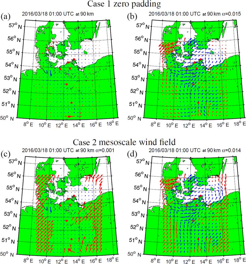
G. Stober et al.: MMARIA winds 4895
larly to the general case (see above). At present we still use is already interpolated to the defined grid cells, further re-
a mean total temporal and vertical shear amplitude for the ferred to as “packed wind retrieval”. The packed retrieval has
whole domain area. In order to take into account that each the advantage that the inversion matrix only scales with the
observed meteor does not occur exactly at the position of the number of grid cells and not with the number of meteors, as
grid point x j , which denotes the center of our grid cells, we is the case for the “full wind retrieval”. The unknown 3-D
assign a weight to each observation (Shepard, 1968), i.e., wind components for each grid cell are also expressed as a
vector
γx
wi (x j , x i ) = . (6)
|x j − x i |p u = [u1 , v1 , w1 , · · ·, um , vm , wm ]T ∈ R3m×1 , (8)
The weight wi for meteor i at position x i and at time ti where m is the number of grid cells. The mapping in Eq. (7)
is inversely proportional to its distance to the center of the can be compactly expressed using the following matrix equa-
grid cell j . The exponent p is used to control how fast the tion:
weight is reduced as a function of distance. Assuming a value
p = 0 results in a box car with equal weight for each meteor v r = Gu, (9)
independent of its distance from the grid cell center. We use
the distance in meters and p = 0.2. The value of p is selected which relates all measured radial velocities to 3-D velocities
in such a way that a meteor at 30 km distance from the grid within a grid. More explicitly, this is
cell center enters the retrieval with a non negligible weight.
..
The term γ is used to control the slope of the space distance,
we use γx = 1.0. The main reason for the averaging is that .
vr,i =
a single meteor, which lasts for 20–200 milliseconds, does
..
not necessarily provide a representative mean wind velocity .
for a 30 min time bin at a grid point or cell. At least two
.. ..
meteors have to occur within one grid cell, otherwise we do . ... ... ... .
.. ..
not attempt to estimate the wind speed for that grid cell. We
. 0 0 0 .
will discuss later how this weight is applied in the inversion
.. ..
procedure. . cos(φi ) sin(θi )
sin(φi ) sin(θi ) cos(θi ) .
We can relate the measured radial velocity of each meteor . ..
..
0 0 0 .
to the three dimensional wind velocity by using local ENU
.. ..
coordinates for each measurement i as follows: . ... ... ... .
..
vr,i = uj cos(φi ) sin(θi ) + vj sin(φi ) sin(θi ) + wj cos(θi ), .
uj
(7)
vj .
(10)
w j
where vr,i is radial velocity for meteor i; uj , vj , and wj are
..
the zonal, meridional, and vertical wind components in grid .
cell j , corresponding to the meteor location. The angles θi
and φi , corresponding to meteor i, are the local ENU coor- The geometry matrix G combines all measurements from
dinates corresponding to the line of sight velocity along the all possible viewing geometries, but it is not directly invert-
direction vector from the radar. In the case of a forward scat- ible. Although we have several different viewing geometries,
ter geometry the measurement of the radial velocity is more we do not get always three independent measurements for
complicated. For multi-static geometries it has to be consid- each grid cell. Hence, the number of unknowns is still larger
ered to obtain the effective Bragg wavelength and pointing than the number of measurements (rows in matrix G). This
vector (see Stober and Chau, 2015). is the case in particular for the edges of our domain area.
The radial wind equation for arbitrary measurements and Ill-posed problems can be solved by adding additional
grid cells can be expressed as a linear matrix equation. The constrains. Very often the smoothness of the unknown pro-
mapping from the zonal, meridional, and vertical compo- vides a reasonable way to regularize an ill-posed problem
nents to observed radial velocities is given by a geometry (Aster et al., 2013). The smoothness in our case corresponds
matrix G ∈ Rn×3m . All the measurements during an analysis to the spatial derivative for each wind component and grid
interval are represented as a vector v r ∈ Rn×1 , where n is the cell. This is equivalent to the assumption that the wind field is
number of measurements. The radial velocity vector v r con- only slightly changing between neighbored grid cells. Hence,
tains all observed radial velocities, either for each individual we define a smoothness matrix L ∈ R3m×3m in such a way
meteor weighted by its distance from the grid cell, further re- that we couple neighbored grid cells for each velocity com-
ferred to as “full wind retrieval”, or an averaged value that ponent separately. For one velocity component, and one grid
www.atmos-meas-tech.net/11/4891/2018/ Atmos. Meas. Tech., 11, 4891–4907, 2018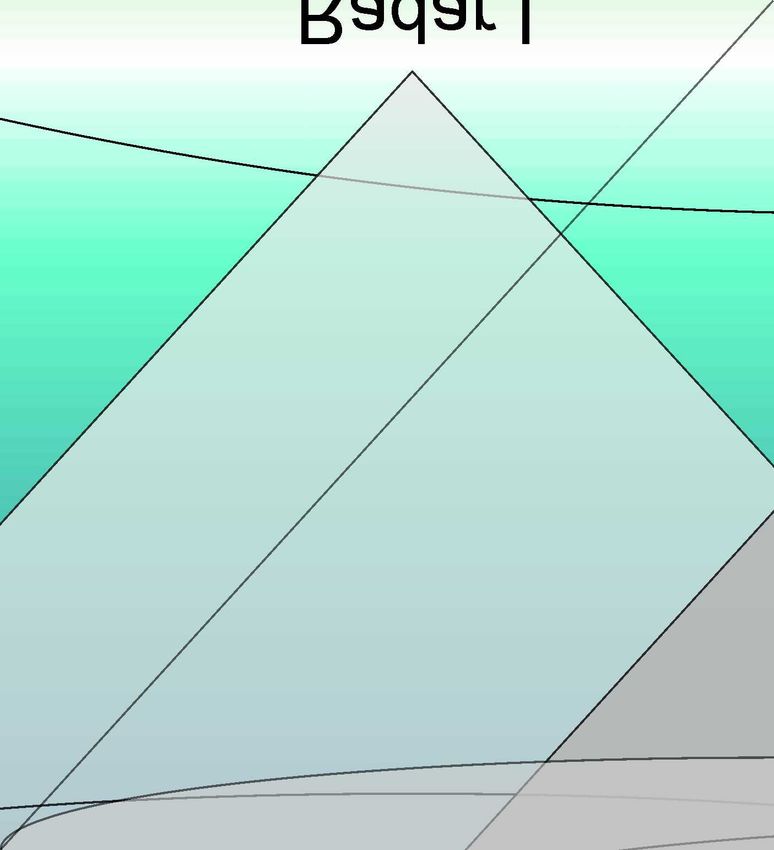
4896 G. Stober et al.: MMARIA winds
regularization uses a rather low regularization strength αmeso ,
which is one order of magnitude smaller than the L regular-
ization for the cases presented here.
Combining all the information and the smoothness con-
straints into a set of equations allows solving the ill-posed
problem. We obtain an estimate for the 3-D wind compo-
nents û at all grid cells solving the equation
û = (GT 6 −1 G + αLT L)−1 GT 6 −1 v r , (12)
which is a standard regularized weighted linear least-
squares estimator (Aster et al., 2013). The matrix 6 =
diag(σ12 , · · ·, σn2 ) is a diagonal matrix that contains the vari-
ance (i.e., measure of uncertainty) given to each measure-
ment σi2 . The regularization parameter α provides a weight
to the regularization constraint. It describes the coupling
strength between neighboring grid cells. It should be noted
Figure 4. Schematic of L matrix for a center grid cell. that a number of alternatives to regularizing the solution also
exist.
In the inversion process the weight 6 −1 consists of contri-
cell, the elements of matrix L would be butions due to the radial velocity uncertainty, the spatial and
temporal weighting functions as outlined above, the angular
..
uncertainties in the measurements of φ and θ and the errors
. 0 0 ... 0 ... 0 ... 0 0
. .. in the zonal, meridional vertical wind components after each
L = .. 4 −1 ... −1 ... −1 ... −1 . (11)
iteration step. There are grid cells where a sufficient num-
..
0 0 0 ... 0 ... 0 ... 0 . ber of measurements is not available (more than 2 meteors
. are required) and only the mesoscale wind field is used. In
this case, the measurement is weighted by a large uncertainty
The matrix L contains such differences for all grid cells (σi = 200 m s−1 ) to ensure that this does not strongly bias the
and all velocity components. The L matrix is constructed that inversion. However, there are areas where ,due to the radial
the total difference between a grid cell and its for neighboring nature of the meteor measurements, the solution can differ
grid cells is small and gradients within the x–y plane are not rather significantly due to the mesoscale regularization.
damped. In Fig. 4, a scheme of how the smoothness matrix In the following we are going to demonstrate the robust-
is constructed is shown. The number of neighbor grid cells ness of our algorithm, independent of the choice of regu-
defines the number of entries in L for each grid cell. larization parameter α and the mesoscale boundary condi-
Finally, we have to deal with grid cells in the domain tions. For simplicity we will only focus on horizontal winds,
area where no measurement is available for a given time– and leave the discussion of vertical mesoscale wind veloc-
altitude bin. This issue is solved by introducing a mesoscale ity for future work. In order to obtain reliable and physically
wind field solution to these grid cells. We tested three pos- meaningful vertical velocities, additional regularization con-
sible mesoscale solutions and checked how much the final straints might be required.
solution depends on this mesoscale boundary condition. The
most trivial way is zero padding or simply not using an ex- 3.3 Robustness of wind field solution
plicit a priori for these grid cells, the second one is estimating
a mean wind using all radial velocity measurements with the Solving Eq. (12) is straightforward using singular value de-
“all-sky” fit and the third possibility is to derive a mesoscale composition or matrix inversion algorithms. As the wind
wind field solution by computing local mean winds for each field inversion is still a linear problem, we just need to find
multi-static geometry and to estimate a distance weighted a proper solution for the regularization parameter α. A large
background wind field for each grid cell. A similar result α means that our solution is dominated by the regularization
is achieved by applying volume velocity processing (VVP) constraint, a too small α results in a too weak coupling be-
(e.g., Browning and Wexler, 1968; Waldteufel and Corbin, tween neighboring grid cells, making the solution unstable
1979), which was already successfully applied using hori- as erratic points start to dominate. This is usually expressed
zontally resolved radial wind measurements (Stober et al., in the so-called “L-curve” (e.g., Aster et al., 2013).
2013) or multi-static SMR observations (Stober and Chau, In Fig. 5, we compare the obtained wind fields for different
2015; Chau et al., 2017). The mesoscale solution is consid- strengths of the regularization parameters α. The left picture
ered in the retrieval as diagonal matrix prescribing a velocity shows what we consider as solution with α = 0.014, which
(zonal, meridional, vertical) for each grid cell. The mesoscale seemed to be sufficient in this case. The wind field in the cen-
Atmos. Meas. Tech., 11, 4891–4907, 2018 www.atmos-meas-tech.net/11/4891/2018/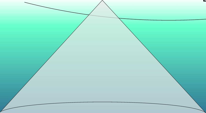
G. Stober et al.: MMARIA winds                                                                                                       4897

Figure 5. Comparison of 2-D wind fields for three different α = 0.014, α = 10, and α = 0.000001. The length of the arrows between the
images does not scale.

                                                                          constant in time, instead of estimating a local regularization
                                                                          strength α for each grid cell. The local approach did not sup-
                                                                          press erratic structures or outliers in the same way, but is go-
                                                                          ing to be further considered as it is going to be beneficial for
                                                                          larger domain areas. After comparing thousands of images
                                                                          using different strengths and ways of estimating the optimal
                                                                          α, it turned out that α = 0.1 is very often a useful value,
                                                                          which leads to a convergence within eight iterations. How-
                                                                          ever, the choice of α depends on the used statistical weights
                                                                          and uncertainties entering the retrieval.
                                                                             As already mentioned above, there are grid cells where we
                                                                          have no direct measurements from one of the systems. We
                                                                          suggested using a mesoscale solution for these points. Now
                                                                          there is the question whether our solution depends on this
                                                                          pre-described mesoscale wind field. Therefore, we prepared
                                                                          two test cases. In the first test, all grid cells with no direct
                                                                          measurements are zero padded. For the second test, we use
                                                                          a computed mesoscale wind field estimated from VVP. Fig-
                                                                          ure 6 shows four pictures using the two test cases. Different
                                                                          colors label grid cells with direct radial velocity measure-
                                                                          ments (blue) and grid cells with the mesoscale solution (red).
                                                                          The left plot displays the first iteration step and the right one
                                                                          shows the finally obtained wind field solution. North of 52◦ N
Figure 6. Comparison of wind field solution in dependence of the
                                                                          there are almost no differences of the solution if one just
background mesoscale solution. (a, b) Test case with zero padding:
first (a) and final iteration (b). (c, d) Test case with mesoscale wind
                                                                          compares the blue arrows. The main reason for this good
field (obtained from the data): first (c) and final iteration (d).        agreement is that almost all points are linked by multiple
                                                                          observing geometries, whereas south of 52◦ N we basically
                                                                          have only monostatic observations. As a result the obtained
                                                                          wind field in the southern part of the domain area is more
ter was computed assuming a much too strong α = 10. This                  prone to be affected by the boundary conditions. However, as
obviously leads to a much too smooth wind field, but still                there is almost no visible difference between the wind fields
keeps some mesoscale wind field structure. A much higher                  at latitudes north of 52◦ N, we conclude that there is almost
value in the order of 100 or 1000 is going to further reduce              no impact on the determined wind fields by the pre-described
the shown variability. The right picture shows an example                 mesoscale winds.
with a regularization constraint of α = 0.000001 that is in-                 Further, we investigated the differences between the full
tentionally much too small. This obviously leads to some er-              wind retrieval and the packed wind retrieval. Therefore, we
ratic structures and outlier solutions begin to dominate the              kept the regularization strength fixed for both retrievals. The
wind field.                                                               packed retrieval makes use of the total wind variances for
   We tested different possibilities to define an optimal reg-            each grid cell and a mesoscale regularization, whereas the
ularization strength α. At present we optimize our solution               full wind retrieval uses each individual radial velocity un-
with a global estimate that is valid for the whole domain and

www.atmos-meas-tech.net/11/4891/2018/                                                       Atmos. Meas. Tech., 11, 4891–4907, 2018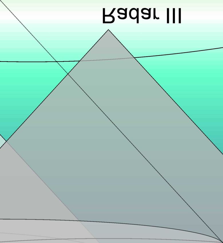
4898                                                                                                      G. Stober et al.: MMARIA winds

Figure 7. Comparison of wind retrievals. Panel (a) shows the solutions of the “packed wind retrieval”. Panel (b) shows the same time and
altitudes for the “full wind retrieval”.

certainty and no explicit mesoscale regularization. The other         Table 1. Technical specifications of the two active meteor radars.
weights and the error treatment is the same. Figure 7 shows
a sequence of three successive time steps for both retrievals.           Parameter                        Juliusruh          Collm
The difference in coverage is because we reduced the limit               frequency (MHz)                  32.55              36.2
for the full wave retrieval to one meteor per cell, which                power Tx (kW)                    30                 15
would be not sufficient for the packed wind retrieval. Fur-              PRF (Hz)                         625                625
ther, the packed wind retrieval indicates the impact of the              range resolution (km)            1.5                1.5
mesoscale solution at the edges of the domain area. How-                 antenna                          crossed dipole     crossed dipole
ever, the general shape of the wind field is reproduced by               operation                        pulsed             pulsed
both approaches with a remarkable agreement. This is fur-                Code                             7-bit Barker       7-bit Barker
ther underlined by a correlation density plot shown in Fig. 8.           location                         54.6◦ N, 13.4◦ E   51.3◦ N, 13.0◦ E
The scattering around the center line is mainly due to the dif-        PRF – pulse repetition frequency
ferent weights and the mesoscale regularization, which was
used in the packed wind retrieval compared to the full wind
retrieval.                                                            scribed in detail in Stober and Chau (2015); Vierinen et al.
                                                                      (2016).
                                                                         In parallel, we also operated a newly developed continu-
4   Horizontally resolved wind fields and initial                     ous wave (CW) coded system that complement our pulsed
    validation                                                        SMR network for one week. The CW-coded prototype was
                                                                      tested from 10–12 June 2015 (Vierinen et al., 2016). The
The above described algorithm is applicable to all types of           first campaign used the existing infrastructure by transmit-
multi-static observations. In 2014 we started to build the            ting from Juliusruh and recieving at Kuehlungsborn. From
MMARIA network in Germany. At present the network con-                14–20 March 2016 there was a second CW-coded campaign
sists of 2 monostatic SMRs (located at Juliusruh 54.6◦ N,             where two temporary transmitters were installed. The trans-
13.4◦ E; and Collm 51.3◦ N, 13.0◦ E; see Table 1). In addi-           mitters were located in Luebs (53.7◦ N, 13.9◦ E) and Schw-
tion to that we installed three receiver-only stations, namely        erin (53.6◦ N, 11.4◦ E), and operated at the same frequency
a dual frequency station in Kuehlungsborn (54.1◦ N, 11.8◦ E)          as the Juliusruh pulsed system, i.e, 32.55 MHz.
and a single frequency station in Juliusruh, i.e., resulting in          During the March campaign in 2016 the multistatic net-
5 different links. Our preliminary results using such obser-          work consisted of two monostatic and five multi-static links.
vations from two links (i.e., Jruh–Jruh, Kborn–Jruh) are de-          Some technical specifications of the experiment settings of

Atmos. Meas. Tech., 11, 4891–4907, 2018                                                      www.atmos-meas-tech.net/11/4891/2018/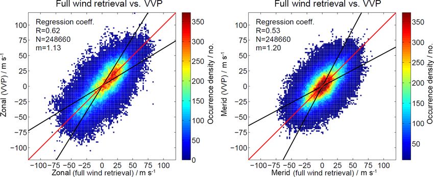
G. Stober et al.: MMARIA winds                                                                                                        4899

Figure 8. Comparison of zonal and meridional winds as derived from the full wind retrieval algorithm and the packed wind retrieval.

the SMRs and the locations of the multi-static links are sum-
marized in Tables 1 and 2, respectively. To simplify the dis-
cussion about the different viewing geometries, we introduce                                                         V

the virtual radar location of each multi-static link (see Fig. 9).
The virtual radar location is defined as the center point of                                        M
the ellipse created by the transmitter and receiver antennas,
which are located in the focal points of this ellipse. The de-
                                                                                               B
rived Doppler velocities are measured with respect to the vir-
tual radar location, or defined by the middle point of the cor-
responding transmitter and receiver link, i.e., projected in the
unit vector of the meteor position and this middle point. The                                           V
resulting MR network is shown in Fig. 10. Panel (a) shows
the position of all used transmitter and receiver sites. Panel
(b) shows the diversity of viewing geometries that results
from the combination of the active radars and the multi-static
links. The red points label either the position of the MRs or          Figure 9. Schematic of a typical forward scatter meteor radar. The
the virtual locations of the multi-static links.                       position of the Tx and Rx are known and all other parts are mea-
   In Fig. 11 we show an overview of the zonal and merid-              sured. The Bragg vector k b always points towards the center of the
                                                                       direction vector d.
ional winds obtained from an all-sky fit as described above.
The campaign was conducted during the transition from win-
ter to summer circulation. The first 3 days are characterized
by a mean westward zonal wind that becomes weaker in the               (< 20 m s−1 ), whereas very smooth wind fields are often re-
second half of the campaign, which is typical for this time            lated to higher wind speeds (> 40 m s−1 ).
of the year (e.g., Wilhelm et al., 2017). The mean meridional             Figure 12 presents two examples of obtained 2-D wind
wind is close to zero. Both wind components indicate a mod-            fields. The domain area was reduced and optimized to cover
erate tidal activity, which is dominated by the semi-diurnal           the Baltic coast where most of multi-static meteor links are
tide with a tidal amplitude of less than 50 m s−1 .                    concentrated. The wind fields are computed using the full
   For the same period we generated three movie sequences              wind retrieval and do not include an explicit mesoscale wind
at 82, 90, 96 km altitude using the full wind retrieval. They          field regularization. The left figure indicates a potential body
show the 2-D wind fields and their temporal evolution with             force of a breaking GW causing an acceleration of the flow
1 h time steps. The movies can be found in the Supplement.             (Vadas and Fritts, 2001). The second example indicates a
The clockwise rotation of vector field is mainly due to the            closed small scale vortex above the Baltic coast. The vor-
semi-diurnal tide. However, the movies also show the tem-              tex is also rather likely the result of a body force event in the
poral and spatial variability due to GWs. The appearance               North East corner of the domain area accelerating the flow
and disappearance of the red points indicates whether this             towards the south west direction.
viewing geometry was available during the inversion or not.               We did also perform an initial validation of the derived
Note that arrows are scaled within each image. As a result             wind field for the complete campaign period through test-
more distorted wind fields are often related to weak winds             ing the consistency of the wind observations compared to the
                                                                       “all-sky” fit and the VVP. A comparison of the mean zonal
                                                                       and meridional winds obtained from the all-sky fit and the

www.atmos-meas-tech.net/11/4891/2018/                                                     Atmos. Meas. Tech., 11, 4891–4907, 2018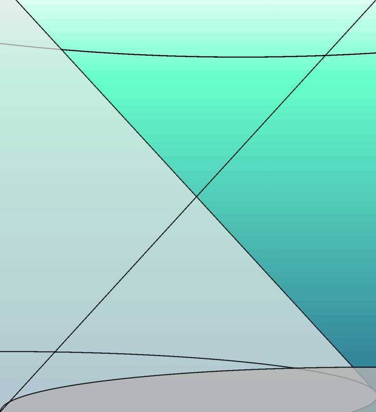
4900                                                                                                           G. Stober et al.: MMARIA winds

Table 2. Technical specification of the multi-static links used in the experiment campaign in March 2016.

          Parameter             Juliusruh–Kborn     Collm–Kborn         Collm–Juliusruh                Luebs–Kborn        Schwerin–Kborn
          location Tx           54.6◦ N, 13.4◦ E    51.3◦ N, 13.0◦ E    51.3◦ N, 13.0◦ E               53.7◦ N, 13.9◦ E   53.6◦ N, 11.4◦ E
          location Rx           54.1◦ N, 11.8◦ E    54.1◦ N, 11.8◦ E    54.6◦ N, 13.4◦ E               54.1◦ N, 11.8◦ E   54.1◦ N, 11.8◦ E
          virtual location      54.4◦ N, 12.6◦ E    52.7◦ N, 12.4◦ E    53.0◦ N, 13.1◦ E               53.9◦ N, 12.8◦ E   53.9◦ N, 11.6◦ E
          frequency (MHz)       32.55               36.2                36.2                           32.55              32.55
          operation principle   pulsed              pulsed              pulsed                         cw                 cw
          transmitted power                                                                            500 W              500 W
          distance (km)         118.6               323.6               370.6                          144.8              58.2

        Kborn – Kuehlungsborn

                                                                                                       MMARIA Germany 2016
                                                                                         120                                                 100

                                                                                                                                                    Zonal / m s -1
                                                                                         110                                                 50

                                                                         Altitude / km
                                                                                         100
                                                                                                                                             0
                                                                                          90
                                                                                          80                                                 −50

                                                                                          70                                                 −100
                                                                                          14/03 15/03 16/03 17/03 18/03 19/03 20/03 21/03

                                                                                         120                                                 100

                                                                                                                                                    Meridional / m s -1
                                                                                         110                                                 50
                                                                         Altitude / km

                                                                                         100
                                                                                                                                             0
Figure 10. (a) Schematic view of multi-static network during the                          90
campaign in March 2016. (b) Geographic map of different viewing                           80                                                 −50
geometries (red points). The shaded areas label a circle of 300 km
                                                                                          70                                                 −100
in diameter around each center of radial velocity measurements.                           14/03 15/03 16/03 17/03 18/03 19/03 20/03 21/03
                                                                                                            Days (dd/mm)

                                                                        Figure 11. Overview of zonal and meridional wind components ap-
mean wind velocities of the full wind retrieval over the do-            plying the standard wind analysis to the MMARIA network during
main area and for all available altitudes between 82–98 km              the March 2016 campaign.
are shown in Fig. 13. The mean wind velocity was obtained
by summation of all grid cells that are constrained by ob-
servations. The comparison shows that there is a remarkable             the small scale structures in the wind field compared to the
agreement between the all-sky fit and the mean 2-D wind ve-             VVP.
locity (full wind retrieval) within the domain area. The cor-
relation is as high as 0.98 for the zonal mean wind and 0.97
for the mean meridional winds. The slightly weaker agree-               5                Obtaining horizontal wavelength spectra
ment of the meridional component is likely related to the in
general lower meridional wind speeds compared to the zonal              The presented full and packed wind retrieval algorithms
winds.                                                                  opens new possibilities to investigate atmospheric dynam-
   We also performed an initial comparison between the VVP              ics. The spatial information seems to be useful to study the
derived wind estimates for each grid point and the 2-D hor-             horizontal wavelength/wavenumber power spectra of kinetic
izontally resolved wind fields, which were again obtained               energy. For the troposphere and lower stratosphere, Nastrom
from the full wind retrieval. We compared all wind veloci-              and Gage (1985) analyzed about 6000 commercial aircraft
ties at all grid cells between 82–98 km altitude. In Fig. 14            flights. They found a spectral slope of k −5/3 for wavelengths
we show the resulting correlation density plot. The correla-            between 2.6 and 400 km, which steepens to k −3 for larger
tion of the zonal and meridional winds are lower compared               wavelengths. The k −5/3 slope is considered to be represen-
to the agreement of the mean winds. The main reason for the             tative for mesoscale GWs, whereas the steeper slope is more
increased scattering is attributed to two effects. Firstly, the         characteristic for the synoptic scale.
VVP uses a linear extrapolation towards the edges of the do-               Due to the regular spatial grid horizontal wavelength spec-
main area, which is not necessarily the best approximation.             tra are easily obtained from the derived horizontally resolved
Secondly, the 2-D full wind retrieval reveals much more of              wind fields. The mean spectrum is computed by adding all

Atmos. Meas. Tech., 11, 4891–4907, 2018                                                                www.atmos-meas-tech.net/11/4891/2018/
G. Stober et al.: MMARIA winds 4901
6 Discussion
Retrieving horizontally resolved wind fields from multi-
static SMR networks at the MLT provides new possibilities
to investigate the intermittency and spatial characteristics of
GWs and vortical modes, which are not yet accessible by
other remote sensing techniques for these spatial scales and
with that temporal resolution. In particular, the wind and its
spatial characteristics are required to understand wave break-
ing and the associated momentum transfer to the background
Figure 12. Two examples of obtained wind fields showing a small
(e.g., Fritts and Alexander, 2003; Fritts et al., 2014).
vortical structure above the Baltic coast and a potential body force A crucial part of the presented wind field analysis, inde-
of a breaking GW. pendent of the choice of the retrieval method, is the spatio-
temporal sampling. Increasing the spatial resolution is only
meaningful if we also decrease the temporal sampling win-
dow. However, with a decreasing number of detections per
grid cell within the domain area the more sparse our wind
field is constrained. This brings us to the question on how
representative an observed radial velocity of an individual
meteor is for our selected time, altitude and spatial resolu-
tion. If we want to resolve small scale structures with char-
acteristic life times of minutes and horizontal scales com-
parable to our grid resolution, e.g., bore events or break-
ing GW (ripples) (Hecht et al., 2007), a much denser MR
network is desirable. However, even with the present stage
Figure 13. Scatter plots of mean zonal and meridional winds ob- of the MMARIA Germany network we are able to resolve
tained from the full wind retrieval and VVP. The mean is computed mesoscale vortical modes as well as GWs. As a result of
as average over the domain area. the spatio-temporal sampling we expect to be more sensitive
to vortical modes and to resolve the effects of body forces
of breaking GW (Vadas and Fritts, 2001). A duplication of
latitudinal cuts through the domain area at a given altitude meteor counts within the domain area would allow to de-
during one day. Considering that the coverage of our 2-D crease the temporal resolution down to 10–15 min compared
wind fields is variable, we included only latitudinal cuts with to the present stage (30–60 min). A significant improvement
more than 12 grid points constrained by measurements. The (15 km×15) of the spatial resolution would require more than
resultant spectra are shown in Fig. 15 and are based on the 4 times the number of counts if the temporal resolution is
full retrieval results. The grey points are obtained by plotting kept the same (30 min).
each individual spectrum. The black line indicates the mean The obtained 2-D wind fields are also ideal to comple-
spectrum. We further added two reference slopes with k −5/3 ment other mesospheric measurements. The combination of
and k −3 . The straight green and black lines are estimated by the horizontally resolved wind fields with other mesospheric
a linear fit and label two different slopes using a wavelength observations like airglow imagers (e.g., Hecht et al., 2007)
window 60–140 km (green) and 140–800 km (black). The or the Advanced Mesospheric Temperature Mapper (Taylor
vertical light blue lines represent the domain boundaries. The et al., 2009; Pautet et al., 2014, 2016) is going to provide a
spectra are estimated by using Lomb–Scargle periodograms more complete picture of the MLT dynamics. The horizon-
(Lomb, 1976; Scargle, 1982). tally resolved wind fields allow a better characterization of
The spectra shown in Fig. 15 suggests that our domain area the mesoscale mean flow. The airglow imagers provide more
has a sufficient large extension to get an idea of the transi- information to small scale structures (a few kilometers).
tion between the k −5/3 to k −3 spectral slopes at the meso- During the past few years, there were also several attempts
sphere. However, we have not yet gathered enough statis- to retrieve horizontally resolved wind fields using Fabry–
tics to pinpoint a transition scale. Typically, the synoptic Perot Interferometer (FPI) in the thermosphere (Meriwether
scale is associated to a more vortical driven flow, whereas et al., 2008; Harding et al., 2015). In particular, Harding et al.
the mesoscale GW flow regime is characterized by divergent (2015) used a comparable retrieval and constrained the wind
modes or GWs. At least for the 5 campaign days there is only field solution by the smoothness and the curvature. They
a weak day-to-day variability. showed data collected above Brazil using up to 7 FPI com-
bined to a FPI network. They obtained rather smooth wind
fields similar to those shown in Fig. 5 (α = 10). A combina-
www.atmos-meas-tech.net/11/4891/2018/ Atmos. Meas. Tech., 11, 4891–4907, 20184902 G. Stober et al.: MMARIA winds
Figure 14. Comparison of zonal and meridional winds as derived from the new retrieval algorithm and the estimates for each grid point
applying VVP.
Wavelength power spectrum (Germany) 18 Mar 2016 at 90 km The introduced packed and full wind retrieval algorithms
4
10 for arbitrary non-homogeneous wind fields show the poten-
tial to investigate mesoscale dynamics at the MLT by em-
Spectral power density / km2 s -1
ploying multi-static SMR networks. Horizontally resolved
3
10 winds open possibilities to study the MLT dynamics. We
demonstrate that our preliminary derived wind fields are suit-
able to obtain horizontal wavelength spectra to access the
2 transition scale between a k −3 to a k −5/3 slope, that has been
10
observed in the troposphere (Nastrom and Gage, 1985).
Horizontally resolved winds at the MLT open new ways to
1 Observed spectrum investigate dynamical processes on scales between hundreds
10 −2.2
Slope n down to a few kilometers. Based on these winds it is going to
Slope n−1.3 be possible to study the momentum transfer of breaking grav-
n−3 (synoptic) scale
n−5/3 gravity wave scale
ity wave in case studies in much more detail. The resolved
0
10 winds are further suitable to obtain a spatially resolved mo-
1000 200 100 60
Horizontal wavelength / km mentum flux, or to measure propagation directions of GW
directly as well as their intrinsic spatial characteristics. The
Figure 15. Horizontal wavelength spectra and estimated slopes to retrieved winds are also usable to complement other mea-
identify the transition from the mesoscale GW to the synoptic scale. surements such as airglow observations combining both data
sets to estimate the intrinsic wave parameters, which are of-
ten not accessible without the knowledge of the background
tion of a FPI and a MR network, in combination with further
winds. At present there is also no other measurement tech-
optimized retrieval algorithms, can enhance our understand-
nique available to observe and study the relative importance
ing of the vertical coupling between the layers and the prop-
of vortical compared to divergent atmospheric modes.
agation of waves, their interaction, and dissipation.
We performed an initial validation of our packed and full
wind retrieval algorithms by comparing the mean winds to
7 Conclusions the standard SMR wind analysis, which shows remarkably
good agreement. Further, we compared the wind fields ob-
After establishing the MMARIA-concept in Stober and Chau tained from VVP, using a gradient extrapolation of the winds
(2015), we extended the SMR network in Germany, which to our grid points with our full wind retrieval solution. This
now consists of two monostatic SMRs at Juliusruh and comparison reveals that both methods provide a good ap-
Collm and three multi-static links between Juliusruh–Kborn, proximation of the mesoscale wind field, but show larger dis-
Collm–Kborn, and Collm–Juliusruh. Further, we investi- crepancies at the smaller scales, which is expected as the 2-D
gated new technological concepts by adding two CW-coded full wind retrieval of 3-D wind vectors is designed to infer
transmitter (Vierinen et al., 2016). Here we present initial such small scale features.
results from a 5 day campaign in March 2016 combining The presented algorithms demonstrate the potential of
pulsed and cw-coded multi-static SMR observations, that re- SMRs to be used as networks. These systems are cheap
sulted in 7 links. enough and sufficiently automated to be deployed at remote
Atmos. Meas. Tech., 11, 4891–4907, 2018 www.atmos-meas-tech.net/11/4891/2018/G. Stober et al.: MMARIA winds 4903
locations and to build rather large networks with several hun- Data availability. The data can be accessed upon request by the
dred kilometers in diameter. Further, the derived packed and authors. Please contact Christoph Jacobi (jacobi@uni-leipzig.de)
full wind retrieval algorithms are applicable to existing data for the Collm meteor radar data. The cw-meteor radar data are
collected from closely co-located SMRs like in Scandinavia available from Jorge L. Chau (chau@iap-kborn.org). The meteor
(Chau et al., 2017). radar data from Juliusruh and Kuehlungsborn can be requested from
Gunter Stober (stober@iap-kborn.de).
www.atmos-meas-tech.net/11/4891/2018/ Atmos. Meas. Tech., 11, 4891–4907, 20184904 G. Stober et al.: MMARIA winds
Appendix A: Coordinate transformations
2
e0 = (a 2 − b2 )/b2 (A3)
In the following we present a short summary of all the coor-
dinate transformations that we used in the presented analysis F = 54b2 z2
scheme. All relevant parameters are listed and the used trans- G = r 2 + (1 − e2 )z2 − e2 (a 2 − b2 )
formation matrices are shown.
c = e4 F r 2 /G3
q
3 p
A1 Geodetic to ECEF s = 1 + c + c2 + 2c
F
P=
The first transformation that we used converts geodetic co- 3(s + 1/s + 1)2 G2
p
ordinates into the ECEF. The geodetic coordinates from the Q = 1 + 2e4 P
radar are given in longitude (λ), latitude (φ), and height s
(z). The height denotes the altitude of the radar above P e2 r a2 1 P (1 − e2 )z2 P r 2
r0 = − + 1+ − −
Earth surface with respect to WGS84 (National Imagery and 1+Q 2 Q Q(1 + Q) 2
Mapping Agency, 2000; Hofmann-Wellenhof et al., 1994). p
2 2 2
The WGS84 defines the semi-major axis of the Earth to U = (r − e r0 ) + z
p
be a = 6 387 137.0 m and a reciprocal of flattening of f = V = (r − e2 r0 )2 + (1 − e2 )z2
1/298.257223563. The semi-minor axis is defined to be b =
b2 z
6 356 752.3142 m. The first eccentricity squared e2 , the sec- z0 =
ond eccentricity squared e0 2 , and the radius of Earth’s curva- aV
ture N is given by
b2
h = U 1−
aV
2
φ = arctan((z + e0 z0 )/r)
e2 = 2 · f − f 2 , (A1)
q
XR 2 +Y2 −X
R R
02
e = (a 2 − b2 )/b2 , λ = 2 arctan
q YR
N = a (1 − e2 sin(φ)2 ). A3 ENU to ECEF
Typically, MR observe meteors at a given distance and direc-
Based on the WGS84 ellipsoid geometry of the Earth any tion relative to its geodetic coordinates. The meteor is given
given geodetic location defined by a longitude, latitude and a in ENU coordinates with respect to the radar location. The
height (height above WGS84 surface) is given by the ECEF up direction is defined by the tangent plane to the Earth’s
coordinates (XR , YR , ZR ) ellipsoid. The meteor position is defined by ENU coordi-
nates (xm , ym , zm ) at a geodetic longitude (λ), latitude (φ),
and height (z). Hence, we have to rotate the ENU-vector
XR = (N + z) · cos(φ) cos(λ), (A2) (xm , ym , zm ) into the ECEF reference (Xm , Ym , Zm ) system
by using the following expression:
YR = (N + z) · cos(φ) sin(λ),
ZR = (N + z − e2 N ) sin(φ). Xm − sin(λ) − sin(φ) cos(λ) cos(φ) cos(λ)
Ym = cos(λ) − sin(φ) sin(λ) cos(φ) sin(λ)
Zm 0 cos(φ) sin(φ)
A2 ECEF to Geodetic xm Xr
· ym + Yr . (A4)
zm Zr
The backward transformation to transform a given coordinate
in ECEF into a geodetic longitude (λ), latitude (φ) and height A4 ECEF to ENU
(z) is more difficult. A summary of possible algorithms is
provided in Zhu (1993). We apply the closed form presented Finally, we want to express our line of sight vector from the
in Heikkinnen (1982). According to Zhu (1993), the average radar towards the meteor in the frame of the ENU coordi-
error is mainly determined by the numerical error introduced nates at the geodetic location of the meteor itself, e.g., the
in the computer, which is in the order of 1 nm. The algorithm line of sight velocity vector is observed at a certain azimuth
presented in Heikkinnen (1982) is valid from the Earth center (az) and zenith (ze) angle relative to the radar, but has a dif-
(z = −6300 km) up to height of geostationary orbits. ferent azimuth (az0 ) and zenith (ze0 ) in the frame of the local
Atmos. Meas. Tech., 11, 4891–4907, 2018 www.atmos-meas-tech.net/11/4891/2018/G. Stober et al.: MMARIA winds 4905
geodetic coordinates of the meteor. Assuming that we know Hence, we obtain a local azimuth az0 and ze0 with respect
the ECEF coordinates of the meteor (Xm , Ym , Zm ), and our to the geodetic position of the meteor, instead of the radar
radar location (XR , YR , ZR ) it is straightforward to compute site
the ENU (x, y, z) by using
az0 = arctan(y/x) (A6)
x − sin(λ) cos(λ) 0 z
y = − sin(φ) cos(λ) − sin(φ) sin(λ) cos(φ) ze0 = arccos p .
x 2 + y 2 + z2
z cos(φ) cos(λ) cos(φ) sin(λ) sin(φ)
Xm − XR
· Ym − YR . (A5)
Zm − ZR
www.atmos-meas-tech.net/11/4891/2018/ Atmos. Meas. Tech., 11, 4891–4907, 20184906 G. Stober et al.: MMARIA winds
The Supplement related to this article is available online Fritts, D. C., Janches, D., and Hocking, W. K.: Southern Ar-
at https://doi.org/10.5194/amt-11-4891-2018-supplement. gentina Agile Meteor Radar: Initial assessment of gravity wave
momentum fluxes, J. Geophys. Res.-Atmos., 115, d19123,
https://doi.org/10.1029/2010JD013891, 2010b.
Fritts, D. C., Janches, D., Hocking, W. K., Mitchell, N. J., and Tay-
lor, M. J.: Assessment of gravity wave momentum flux mea-
Author contributions. The manuscript was prepared from GS with surement capabilities by meteor radars having different transmit-
contributions from all co-authors. The source codes of the presented ter power and antenna configurations, J. Geophys. Res.-Atmos.,
wind retrievals are developed by GS. JV and JLC developed the 117, d10108, https://doi.org/10.1029/2011JD017174, 2012.
CW-experiments and carried them out. CJ helped with the data in- Fritts, D. C., Pautet, P.-D., Bossert, K., Taylor, M. J.,
terpretation and ensured the operation of the Collm meteor radar. Williams, B. P., Iimura, H., Yuan, T., Mitchell, N. J.,
SW contributed to the mean wind analysis for the shown wind com- and Stober, G.: Quantifying gravity wave momentum fluxes
parisons. with Mesosphere Temperature Mappers and correlative in-
strumentation, J. Geophys. Res.-Atmos., 119, 13583–13603,
https://doi.org/10.1002/2014JD022150, 2014.
Competing interests. The authors declare that they have no conflict Hall, C. M., Aso, T., Tsutsumi, M., Nozawa, S., Manson, A. H.,
of interest. and Meek, C. E.: A comparison of mesosphere and lower
thermosphere neutral winds as determined by meteor and
medium-frequency radar at 70◦ N, Radio Sci., 40, rS4001,
Acknowledgements. We acknowledge the technical support of our https://doi.org/10.1029/2004RS003102, 2005.
radar systems by Falk Kaiser, Dieter Keuer, Jörg Trautner, and Harding, B. J., Makela, J. J., and Meriwether, J. W.: Estimation
Thomas Barth. We are grateful for the support provided by Sven of mesoscale thermospheric wind structure using a network
Geese, Nico Pfeffer, and Matthias Claßen in developing, deploying, of interferometers, J. Geophys. Res.-Space, 120, 3928–3940,
and operating the CW-coded radars. We thank both reviewers for https://doi.org/10.1002/2015JA021025, 2015.
their help improving our manuscript. Hecht, J. H., Fricke-Begemann, C., Walterscheid, R. L.,
and Höffner, J.: Observations of the breakdown of
Edited by: Markus Rapp an atmospheric gravity wave near the cold summer
Reviewed by: two anonymous referees mesopause at 54N, Geophys. Rese. Lett., 27, 879–882,
https://doi.org/10.1029/1999GL010792, 2000.
Hecht, J. H., Liu, A. Z., Walterscheid, R. L., Franke, S. J., Rudy,
R. J., Taylor, M. J., and Pautet, P.-D.: Characteristics of short-
References period wavelike features near 87 km altitude from airglow and
lidar observations over Maui, J. Geophys. Res.-Atmos., 112,
Aster, R. C., Borchers, B., and Thurber, C. H.: Parameter Estimation d16101, https://doi.org/10.1029/2006JD008148, 2007.
and Inverse Problems, 2 Edn., Academic Press, Boston, 2013. Heikkinnen, M.: Geschlossene Formeln zur Berechnung räumlicher
Becker, E.: Dynamical Control of the Middle Atmosphere, Space geodätischer Koordinaten aus rechtwinkligen Koordinaten, Z.
Sci. Rev., 168, 283–314, https://doi.org/10.1007/s11214-011- Ermess., 107, 207–2011, 1982.
9841-5, 2012. Hocking, W., Fuller, B., and Vandepeer, B.: Real-time deter-
Browning, K. and Wexler, R.: The Determination of Kinematic mination of meteor-related parameters utilizing modern dig-
Properties of a Wind field Using Doppler Radar, J. App. Me- ital technology, J. Atmos. Sol.-Terr. Phy., 63, 155–169,
teorol., 7, 105–113, 1968. https://doi.org/10.1016/S1364-6826(00)00138-3, 2001.
Chau, J. L., Stober, G., Hall, C. M., Tsutsumi, M., Laskar, Hocking, W. K.: A new approach to momentum flux determinations
F. I., and Hoffmann, P.: Polar mesospheric horizontal di- using SKiYMET meteor radars, Ann. Geophys., 23, 2433–2439,
vergence and relative vorticity measurements using mul- https://doi.org/10.5194/angeo-23-2433-2005, 2005.
tiple specular meteor radars, Radio Sci., 52, 811–828, Hofmann-Wellenhof, B., Lichtenegger, H., and Collins, J.: Global
https://doi.org/10.1002/2016RS006225, 2017. Positioning System: theory and practice, Springer-Verlag, Vi-
de Wit, R. J., Hibbins, R. E., Espy, P. J., Orsolini, Y. J., Limpasu- enna, 1994.
van, V., and Kinnison, D. E.: Observations of gravity wave forc- Holdsworth, D. A., Reid, I. M., and Cervera, M. A.: Buckland
ing of the mesopause region during the January 2013 major Sud- Park all-sky interferometric meteor radar, Radio Sci., 39, rS5009,
den Stratospheric Warming, Geophys. Res. Lett., 41, 4745–4752, https://doi.org/10.1029/2003RS003014, 2004.
https://doi.org/10.1002/2014GL060501, 2014. Jacobi, C.: Meteor radar measurements of mean winds and
Elford, W. G.: A study of winds between 80 and 100 km in medium tides over Collm (51.3◦ N, 13◦ E) and comparison with LF
latitudes, Planetary Space Sci., 1, 94–101, 1959. drift measurements 2005–2007, Adv. Radio Sci., 9, 335–341,
Fritts, D. and Alexander, M. J.: Gravity wave dynamics and https://doi.org/10.5194/ars-9-335-2011, 2011.
effects in the middle atmosphere, Rev. Geophys., 41, 1–64, Jacobi, C., Arras, C., Kürschner, D., Singer, W., Hoffmann,
https://doi.org/10.1029/2001RG000106, 2003. P., and Keuer, D.: Comparison of mesopause region meteor
Fritts, D. C., Janches, D., and Hocking, W. K.: Southern Ar- radar winds, medium frequency radar winds and low fre-
gentina Agile Meteor Radar: Initial assessment of gravity wave quency drifts over Germany, Adv. Space Res., 43, 247–252,
momentum fluxes, J. Geophys. Res.-Atmos., 115, d19123, https://doi.org/10.1016/j.asr.2008.05.009, 2009.
https://doi.org/10.1029/2010JD013891, 2010a.
Atmos. Meas. Tech., 11, 4891–4907, 2018 www.atmos-meas-tech.net/11/4891/2018/You can also read