Footprint-scale cloud type mixtures and their impacts on Atmospheric Infrared Sounder cloud property retrievals - Atmos. Meas. Tech
←
→
Page content transcription
If your browser does not render page correctly, please read the page content below
Atmos. Meas. Tech., 12, 4361–4377, 2019
https://doi.org/10.5194/amt-12-4361-2019
© Author(s) 2019. This work is distributed under
the Creative Commons Attribution 4.0 License.

Footprint-scale cloud type mixtures and their impacts on
Atmospheric Infrared Sounder cloud property retrievals
Alexandre Guillaume, Brian H. Kahn, Eric J. Fetzer, Qing Yue, Gerald J. Manipon, Brian D. Wilson, and Hook Hua
Jet Propulsion Laboratory, California Institute of Technology, Pasadena, 91109, USA

Correspondence: Alexandre Guillaume (alexandre.guillaume@jpl.nasa.gov)

Received: 28 November 2018 – Discussion started: 18 December 2018
Revised: 11 June 2019 – Accepted: 13 June 2019 – Published: 14 August 2019

Abstract. A method is described to classify cloud mix-            1   Introduction
tures of cloud top types, termed cloud scenes, using cloud
type classification derived from the CloudSat radar (2B-          There is increasing evidence of secular cloud trends at re-
CLDCLASS). The scale dependence of the cloud scenes is            gional and global scales in both satellite observations (e.g.,
quantified. For spatial scales at 45 km (15 km), only 18 (10)     Norris et al., 2016) and climate general circulation model
out of 256 possible cloud scenes account for 90 % of all ob-      (GCM) simulations (e.g., Zelinka et al., 2013). The pole-
servations and contain one, two, or three cloud types. The        ward migration of the extratropical storm tracks (Barnes and
number of possible cloud scenes is shown to depend on spa-        Polvani, 2013) is coupled to systematic changes in cloud-
tial scale with a maximum number of 210 out of 256 possible       thermodynamic-phase partitioning in forced CO2 experi-
scenes at a scale of 105 km and fewer cloud scenes at smaller     ments in climate GCMs (e.g., Mitchell et al., 1989; Ceppi
and larger scales. The cloud scenes are used to assess the        et al., 2016). The spread in equilibrium climate sensitivity is
characteristics of spatially collocated Atmospheric Infrared      also tightly coupled to the temporal evolution of phase parti-
Sounder (AIRS) thermodynamic-phase and ice cloud prop-            tioning in most climate GCMs (Tan et al., 2016). Obtaining
erty retrievals within scenes of varying cloud type complex-      reasonable observational estimates of the small-scale cloud-
ity. The likelihood of ice and liquid-phase detection strongly    phase partitioning at model subgrid scales is critical for con-
depends on the CloudSat-identified cloud scene type collo-        straining the highly uncertain Wegener–Bergeron–Findeisen
cated with the AIRS footprint. Cloud scenes primarily con-        timescale parameter that is crucial for modeling mixed-phase
sisting of cirrus, nimbostratus, altostratus, and deep convec-    cloud and precipitation processes (Tan and Storelvmo, 2016).
tion are dominated by ice-phase detection, while stratocumu-      A new generation of probability-distribution-function-based
lus, cumulus, and altocumulus are dominated by liquid- and        parameterizations has shown promise for improving climate
undetermined-phase detection. Ice cloud particle size and op-     model simulations of cloud properties (e.g., Golaz et al.,
tical thickness are largest for cloud scenes containing deep      2002) and would benefit from further exploitation of the in-
convection and cumulus and are smallest for cirrus. Cloud         formation available in pixel-scale satellite observations. A
scenes with multiple cloud types have small reductions in in-     rigorous assessment of the scale dependence of cloud types,
formation content and slightly higher residuals of observed       and their mixtures, would also enhance climate GCM eval-
and modeled radiance compared to cloud scenes with sin-           uation and parameterization development research efforts
gle cloud types. These results will help advance the develop-     (Bony et al., 2006).
ment of temperature, specific humidity, and cloud property           Kahn et al. (2018) showed that Atmospheric Infrared
retrievals from hyperspectral infrared sounders that include      Sounder (AIRS) observations of ice cloud optical thickness
cloud microphysics in forward radiative transfer models.          (τi ) and effective radius (rei ) exhibit statistically significant
                                                                  temporal trends that are dependent on latitude and cloud type.
                                                                  Trends in Multi-angle Imaging SpectroRadiometer (MISR)
Copyright statement. © 2019 California Institute of Technology.   observations of cloud texture have suggested that recent thin-
Government sponsorship acknowledged.                              ning of tropical cirrus has led to increased detection of trade

Published by Copernicus Publications on behalf of the European Geosciences Union.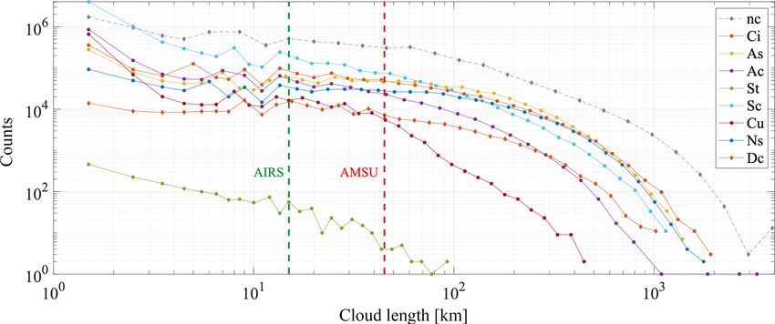
4362                                                                  A. Guillaume et al.: Footprint-scale cloud type mixtures

cumulus (Zhao et al., 2016). Using high-spatial-resolution           2     Data and methodology
estimates of cloud thermodynamic phase obtained from the
Hyperion instrument on Earth Observing 1 (EO-1), Thomp-              2.1    CloudSat and AIRS pixel-scale matching
son et al. (2018) showed that phase mixtures are highly vari-
able at scales smaller than the AIRS footprint or typical GCM        The AIRS/AMSU/CloudSat matchup product described in
grid boxes. These studies (and many others) suggest that             Manipon et al. (2016) is used by Yue et al. (2013) and in this
quantification of the scale dependence of cloud type mixtures        investigation. The matchup process uses a nearest-neighbor
could help explain satellite observations of cloud trends.           approach to geolocate all CloudSat profiles within either an
   Statistical classification methods are commonly used to           AMSU FOR at 45 km spatial resolution at nadir view or a sin-
define weather states or cloud types (e.g., Rossow et al.,           gle AIRS footprint at 15 km spatial resolution at nadir view
2005; Xu et al., 2005; Sassen and Wang, 2008; Wang et                (Kahn et al., 2008). Approximately 45 to 50 (15–17) Cloud-
al., 2016). For instance, joint histograms of cloud top pres-        Sat profiles coincide with a single AMSU FOR (AIRS foot-
sure and optical thickness from the International Satellite          print), in a swath of width 30 FORs (90 footprints). The cloud
Cloud Climatology Project (ISCCP; Rossow and Schiffer,               scenes are first defined at the AMSU FOR scale and are then
1999) are useful for relating cloud types to dynamical, radia-       extended to other spatial scales. We use a 2-year period of
tion, and precipitation variability, as well as in evaluating cli-   data extending from 1 July 2006 until 30 June 2008 which
mate model simulations (e.g., Klein and Jakob, 1999; Jakob           contains about 8 million AMSU FORs (or 24 million AIRS
and Tselioudis, 2003; Rossow et al., 2005; Tselioudis et al.,        footprints).
2013). Weather states are typically mixtures of conventional
cloud types as shown by Rossow et al. (2005) and Oreopou-            2.2    CloudSat cloud types and their mixtures within the
los et al. (2014). Partly inspired by this methodology, we in-              AIRS footprint
troduce the concept of cloud scenes that are defined to be
mixtures of CloudSat cloud types (2B-CLDCLASS; Sassen                The CloudSat 2B-CLDCLASS product is used in this work
and Wang, 2005) that vary with horizontal scale.                     and the algorithm is described in Sassen and Wang (2005,
   As cloud scenes will be matched to coincident A-Train             2008). As summarized in Sassen and Wang (2008) and pre-
observations, we begin by defining cloud scenes with                 vious works, the algorithm uses methods developed from
cloud types derived from CloudSat and observed within                ground-based multiple remote sensors that have been tested
an AIRS/Advanced Microwave Sounding Unit (AMSU)                      against surface observer-based cloud typing reports. The
(Chahine et al., 2006) field of regard (FOR) of roughly 45 km        cloud classification occurs in two steps. First, a clustering
resolution. One AMSU FOR within an AMSU swath is spa-                analysis is performed to group cloud profiles into cloud clus-
tially and temporally coincident with a “curtain” of 94 GHz          ters. Secondly, classification methods are used to classify
CloudSat radar profiles. The likelihood of observing clouds          clouds into different cloud types. The decision trees guiding
is resolution-dependent and is approximately 80 %–85 % at            the classification are complex and are based on 23 variables
the AIRS footprint scale of 15 km (Krijger et al., 2007;             derived from the clustering analysis of the first stage. Geo-
Kahn et al., 2008). The clouds in AMSU sounding FORs                 metric quantities such as cloud base, top, and horizontal ex-
or AIRS footprints are more often broken or transparent and          tents are present in decision trees (Sassen and Wang, 2005).
less often uniform or opaque. Yue et al. (2013) showed that          Plan view and zonal average frequencies of 2B-CLDCLASS
about 43 % of the AMSU FORs are mixtures of CloudSat-                cloud types at its native resolution are reported in Sassen and
identified cloud types, implying that roughly half of cloudy         Wang (2008).
soundings contain mixtures of cloud types.                              There are eight CloudSat-defined classes in the 2B-
   Our purpose in this work is to quantify the scale depen-          CLDCLASS files: cumulus (Cu), stratocumulus (Sc), stratus
dence of cloud type mixtures that are then used to understand        (St), altocumulus (Ac), altostratus (As), nimbostratus (Ns),
the cloud complexity within AIRS cloud-phase and ice cloud           cirrus (Ci), and deep convective (Dc) clouds, with a ninth
property data sets. The AIRS and CloudSat data and the col-          classification of clear sky designated no cloud (nc). Since
location approach are described in Sect. 2. To quantify cloud        each AMSU FOR contains roughly 50 CloudSat profiles
type distributions and their dependence on horizontal scales,        with 125 vertical levels each, there are 950×125 possible dis-
the cloud scenes are first characterized at the AMSU FOR             tinct cloud type combinations (although in practice there are
resolution in Sect. 3.1, are extended to larger and smaller          fewer as many levels reside in the stratosphere) for each
scales in Sect. 3.2, and key results of the scale dependence         AMSU FOR. This number is too high to derive a classifica-
are placed into context in Sect. 3.3. The cloud scenes are           tion that could be useful, i.e., where each cloud type combi-
used to partition AIRS cloud property retrievals into cloud          nation could be populated with a significant number of sam-
types, specifically, cloud-thermodynamic-phase histograms            ples for any climatological study. One particularly appealing
in Sect. 4.2, and mean values of ice cloud microphysical pa-         way to reduce the dimensionality is to limit consideration of
rameters are described in Sect. 4.3. A discussion, summary,          cloud type to cloud top only. This simplification is consistent
and suggestions for future investigation are found in Sect. 5.       with the capabilities of infrared sounders as the sampling of

Atmos. Meas. Tech., 12, 4361–4377, 2019                                                www.atmos-meas-tech.net/12/4361/2019/
A. Guillaume et al.: Footprint-scale cloud type mixtures                                                                        4363

temperature and specific humidity is maximized in the at-           viewing passive infrared sounders. Therefore, we consider
mosphere near and above cloud top, assuming the cloud is            the approach outlined above to be an appropriate compro-
opaque and covers the entire sounder pixel area. There are          mise that retains the diversity of cloud scenes and makes the
950 possible cloud combinations defined in this manner, in-         necessary data processing tractable by reducing the dimen-
cluding clear sky profiles. As a point of comparison, there are     sionality for ease of interpretation.
about 324 000 AIRS soundings per day or about 108 per year.            Lastly, the results of Kahn et al. (2018) suggest larger ice
Even when considering the 16 years of AIRS nominal oper-            cloud particle sizes occur at convective cloud tops compared
ation, the number of cloud type combinations 950 , or about         to thin cirrus at the same cloud top temperature. Given the
5 × 1047 , is many orders of magnitude greater than the num-        key assumption of cloud typing only at cloud top, the 2B-
ber of AMSU FORs available, making it impossible to per-            CLDCLASS product is better suited for identifying convec-
form a statistically significant sampling of all combinations.      tive clouds in AIRS apart from stratiform clouds, the latter
This necessitates further assumptions to define a practical yet     of which are dominant in 2B-CLDCLASS-LIDAR. If 2B-
meaningful set of cloud scenes.                                     CLDCLASS-LIDAR was used in place of 2B-CLDCLASS,
   Two additional simplifications are made here: variations         the statistics would be weighted towards the detection of
in the count of each CloudSat cloud type are not consid-            vast areas of cirrus in thin layers above and in proximity
ered, and the observation sequence of successive cloud types        to convective clouds. The Ci classification dominates in 2B-
is disregarded. These two simplifications are applied to the        CLDCLASS-LIDAR at cloud top and will blur the signals of
AMSU field of view (FOV). We define a cloud scene as a              underlying cumulus and deep convective cloud types that are
list of the cloud types that are present within a given AMSU        capped by thin cirrus.
FOR. For example, the notation (Ci, Ac, Sc, Cu) is used to la-
bel a cloud scene that contains cirrus, altocumulus, stratocu-      2.3   AIRS thermodynamic-phase and ice cloud
mulus, and cumulus clouds at cloud top in any frequency and               properties
in any sequence along the orbit segment. These simplifica-
tions greatly reduce the dimensionality of the classification       The AIRS version 6 cloud-thermodynamic-phase and ice
problem and make cloud scene identification tractable. We           cloud properties (Kahn et al., 2014) are geolocated to the
will show both partly cloudy and completely cloudy scenes           CloudSat ground track and are binned by cloud scene. The
in Section 4, so the clear sky (nc) type is both included and       cloud-thermodynamic-phase algorithm includes two liquid
excluded in the analyses. Since each of the eight cloud types       tests and four ice tests of brightness temperature (Tb ) thresh-
is either present or absent, a cloud scene can also be repre-       olds and Tb differences (1Tb ) in the midinfrared atmospheric
sented by an 8 bit binary string. As a consequence, there are       windows. The Tb and 1Tb thresholds are designed to ex-
256 (28 ) possible cloud scenes that remain after taking into       ploit spectral differences in liquid and ice water indices of
account the aforementioned simplifications. The number of           refraction. The two liquid and four ice tests are each as-
possible cloud scenes is therefore reduced from 950×125 to a        signed a value of −1 and +1, respectively, and a summed
much more tractable 256. The limitations of this approach are       value that ranges from −2 to +4 is reported. Summed val-
(i) a consideration of cloud tops only, (ii) the spatial sequence   ues −2 or −1 indicate liquid clouds, 0 is undetermined, and
and frequency of individual cloud types are not considered,         values ≥ +1 indicate ice, with the highest values indicat-
and (iii) equal weight is given to all cloud types within a         ing deeper, convective ice clouds (Naud and Kahn, 2015).
cloud scene regardless of counts.                                   Ice is detected in 26.5 % of AIRS footprints by Kahn et
   One advantage of using a classification to define cloud          al. (2014), and pixel-scale comparisons with estimates of ice
mixtures rather than an unsupervised learning technique,            from the Cloud-Aerosol Lidar and Infrared Pathfinder Satel-
such as clustering, is that the size of the set of possible cloud   lite Observation (CALIPSO) lidar (Jin and Nasiri, 2014) are
mixtures is well defined and finite (here it is 256). A related     in agreement with AIRS more than 90 % of the time. The
and important advantage of classification is that one can use       success rate, however, is smaller for liquid cloud detection
this set of classes (cloud scenes) with any parameter matched       with AIRS using CALIPSO as a benchmark because of the
to any given scene. Here, the spatial-scale dependence of           small thermal contrast between low-lying liquid clouds and
those cloud scenes is described in Sect. 3.2.                       the surface. Despite this limitation in sensitivity, AIRS rarely
   An alternative approach may consider the vertical layer-         misidentifies liquid clouds as ice (Jin and Nasiri, 2014). Fur-
ing of cloud types or cloud features, some form of weighting        thermore, many liquid clouds are classified as undetermined
based on counts of each cloud type, or possibly the sequence        phase. Low-latitude shallow trade cumulus clouds generally
of cloud types, which may result in different radiance mea-         fall within this category (Kahn et al., 2017).
surements observed by the AIRS instrument (the radiance                Kahn et al. (2014) describe a retrieval algorithm that is
emitted within an AIRS footprint is nonuniform and channel-         based on optimal estimation (OE) theory and derives ice
dependent, as described in Schreier et al., 2010). However,         cloud optical thickness (τi ) and effective radius (rei ) for AIRS
the simplified approach outlined above is broadly consistent        footprints containing ice. The AIRS retrieval sample includes
with the sensitivity and sampling characteristics of nadir-         nearly all ice clouds with τi > 0.1, while the maximum values

www.atmos-meas-tech.net/12/4361/2019/                                                 Atmos. Meas. Tech., 12, 4361–4377, 2019
4364 A. Guillaume et al.: Footprint-scale cloud type mixtures
of τi asymptote to values around 6–8 (e.g., Kahn et al., 2015). The relative ranking of cloud scenes within the AIRS FOV
Scalar averaging kernels (AKs), χ 2 residuals from observed along the CloudSat track is shown in Fig. 1b for the same
and simulated radiance fits, and values of relative error are sets of matched pixels. A total of 10 cloud scenes account
also reported (Kahn et al., 2014). Values of AKs closer to 1.0 for 90 % of all observed cloud scenes (Fig. 1b). This shows
suggest higher information content, while larger relative er- that fewer cloud scenes are found at the smaller AIRS FOV
ror estimates and values of χ 2 indicate increased uncertainty compared to the AMSU FOR.
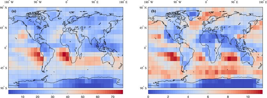
in retrieved parameters. Only the relative magnitude of er- Figure 2 depicts the geographic distribution of Sc at the
ror estimates should be considered since temperature, spe- AMSU FOR scale, the most observed scene after clear sky
cific humidity, surface temperature, surface emissivity, and (nc), and (Ac, Sc) is the most observed mixed cloud scene.
ice crystal habit and size distribution uncertainties are not in- The Sc classification is consistent with the prevalence of stra-
cluded in the error covariance matrices of the AIRS version tocumulus clouds in subtropical subsidence regions and trade
6 algorithm (see Kahn et al., 2014). We focus on the differ- cumulus in the tropics and subtropics (e.g., Yue et al., 2011).
ences in error estimates and χ 2 among cloud scenes and de- The (Ac, Sc) cloud scene is identified most frequently in the
termine which cloud scenes contain higher or lower certainty extratropical storm tracks and the transition from shallow cu-
in their ice cloud properties relative to other scenes. mulus to deep tropical convection.
3.2 Cloud scenes at 1 to 1000 km scales
3 Classification and characteristics of cloud scenes In Sect. 3.1, the relative frequencies of cloud scenes were
derived for exact collocated matches of AIRS and AMSU
3.1 Cloud scenes with ∼ 45 km resolution observations to the CloudSat ground track. As the CloudSat
ground track can oscillate across several AIRS FOVs over
A cloud scene is assigned to every AMSU FOR along the a scan line within a given orbit, the numbers of coincident
CloudSat viewing path using the methodology outlined in CloudSat profiles matching to AIRS and AMSU will vary.
Sect. 2. Using the 2 years of data, a total of 194 out of 256 Below, cloud scenes are derived independently of the specific
possible cloud scenes are observed but only 18 of the cloud AIRS and AMSU collocation geometry.
scenes account for 90 % of all observed scenes (Fig. 1a). The To investigate the scale dependence of the number of cloud
four most common scenes contain one cloud type with or scenes, the approach described in Sect. 2 is modified for a
without clear sky, and the most common mixed cloud scene range of horizontal extents between 1.1 and 1000 km. The
(Ac, Sc) is ranked as the fifth most common scene over- number of observed cloud scenes calculated at each horizon-
all. Intuitively, the more diverse a scene, the less frequently tal scale is shown in Fig. 3a for 10 to 1000 km. At the finest
it should be observed. The scene that ranked last (18th) in scale of 1.1 km, only eight possible observed cloud scenes or
Fig. 1a is (Ci, Ac, Sc). The least frequently observed cloud clear sky are expected. When the scale increases, as expected,
scene with a ranking of 194 contains six cloud types (Ci, As, the number of cloud scenes quickly increases with a total of
Ac, St, Cu, Ns) and was observed only once in 2 years. Of 143 cloud scenes observed at a scale of 11 km. As horizontal
the 256 possible types of cloud scenes, the number of unob- scale is further increased, the probability of observing cloud
served cloud scenes is 62, of which 61 include St. The un- scenes with only one or two cloud types is reduced. After a
observed cloud scenes include the only possible cloud scene maximum number of cloud scenes is obtained at 105 km, the
with eight cloud types together and the seven possible cloud number of cloud scenes will decrease with increasing scale
scenes with seven cloud types together. (e.g., 163 cloud scenes at 990 km) until a limiting case is
The unobserved scenes in the 2-year period contain a me- reached at the largest scale with only one cloud scene with all
dian of five different cloud types. This is consistent with the observed cloud types. The number of cloud scenes observed
improbability of particular cloud types occurring in rapid at least once at the AMSU FOR horizontal scale (indicated
succession over a few tens of kilometers. The only unob- by the red vertical line on Fig. 3a) is approximately 190.
served cloud scene that does not contain St is (Sc, Cu, Ns, The 90th percentile calculated at all horizontal scales is
Dc) and is consistent with the conclusion by Sassen and shown in Fig. 3b. The 90th percentile of the maximum num-
Wang (2008) that Dc (1.8 %) and Cu (1.7 %) clouds are the ber of cloud scenes is 33 between 303 and 440 km in horizon-
least frequent of the cloud types. While Dc and Ns are typi- tal scale. The number at the nominal 45 km AMSU footprint
cally associated with different climatological regimes (trop- scale is 16 cloud scenes, while the average number at the
ical convection versus extratropical storm tracks), occasion- AIRS footprint is 9 cloud scenes. (Note that these are slightly
ally, Dc is embedded within extratropical cyclones and Ns is smaller than values of 18 and 10 using the exact AMSU and
classified in stratiform regions of mesoscale convective sys- AIRS geometry, respectively, in Sect. 3.1.) While these re-
tems (MCSs). Given the prevalence of Sc and Cu in Fig. 1a, sults show that fewer cloud type mixtures are observed at a
it is somewhat surprising that the combination (Sc, Cu, Ns, decreasing length of 45 to 15 km, a variety of cloud type mix-
Dc) is not observed. tures is still encountered. While infrared sounding at 15 km
Atmos. Meas. Tech., 12, 4361–4377, 2019 www.atmos-meas-tech.net/12/4361/2019/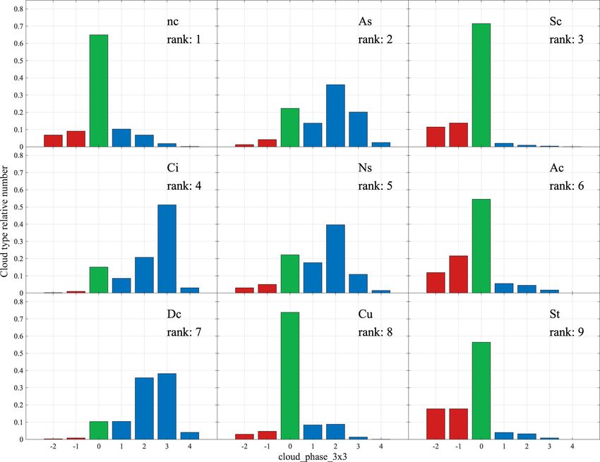
A. Guillaume et al.: Footprint-scale cloud type mixtures                                                                                4365

Figure 1. Histogram of cloud scenes containing relative counts of occurrence observed at the AMSU FOR and AIRS FOV resolution (∼ 45
and ∼ 15 km respectively). The cumulative sum of the relative counts of these 18 (10) cloud scenes amounts to more than 90 % of all cloud
scenes observed globally over a period of 2 years at AMSU (AIRS) resolution.

Figure 2. Geographic distribution of cloud scenes (Sc) and (Ac, Sc) in panels (a) and (b) respectively, in units of percentage with respect to
all of the (194) observed cloud scenes. These scenes were observed at the AMSU FOR resolution (∼ 45 km). Similar plots of the AIRS FOV
resolution (∼ 15 km) are nearly identical (not shown).

resolution does not eliminate the cloud scene complexity en-             3.3    Generalizing to all scales
countered for combined infrared and microwave sounding at
45 km, the vast majority of 15 km footprints contain a smaller           The goal of this section is to derive cloud scene scale statis-
subset of possible cloud mixtures. In Sect. 4, we will deter-            tics that are independent of any regular grid resolution and
mine whether individual cloud types or cloud type mixtures               explore whether these statistics can explain some features
have meaningful impacts on AIRS cloud property retrievals.               of the number of scenes as a function of scale observed in
(Impacts on temperature and specific humidity soundings are              the previous section. In particular, we explore whether these
beyond the scope of this investigation.)                                 statistics can explain the maximum observed around 105 km.
   The reasons for the maximum number of observed cloud                  There is however an inherent difficulty in defining the bound-
scenes (210) at a particular horizontal scale (105 km) are not           aries that delimit any given cloud scene in the absence of a
immediately clear. The scale preference depends on the phys-             predefined horizontal extent. It is possible that within a given
ical characteristics of cloud regimes and the degree to which            cloud scene there exists several scenes with the same cloud
cloud types are mixed together by region and furthermore de-             types but differing lengths making the scene identification
pend on cloud length distributions (Guillaume et al., 2018). A           ambiguous. To circumvent this problem, we define a cloud
simple model is described below that is able to approximate              scene and its maximum length as follows.
the results of Fig. 3 and offers some insight for the observed             1. We search for a cloud scene containing a predefined
maximum frequency of cloud scenes and the spatial scale at                    mixture of cloud types. The spatial extent of this scene
which it occurs.                                                              is delimited by cloud types (or clear sky) on both ends
                                                                              that do not belong to the mixture.

www.atmos-meas-tech.net/12/4361/2019/                                                        Atmos. Meas. Tech., 12, 4361–4377, 2019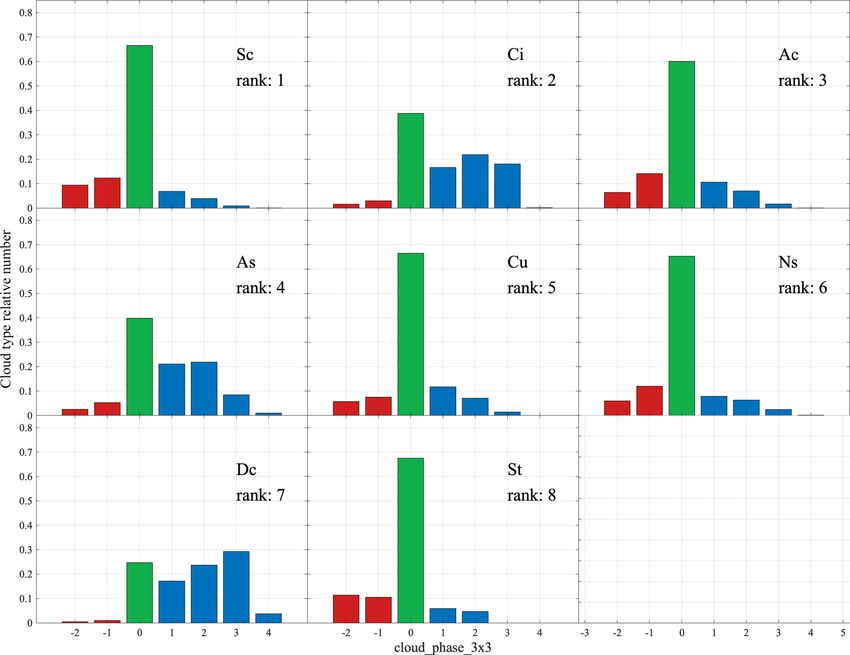
4366                                                                                          A. Guillaume et al.: Footprint-scale cloud type mixtures

                                                                                                 Before steps (1) and (2) are used to quantify the maxi-
                                                                                             mum and minimum lengths for each of the 247 mixed scenes
                                                                                             (256 minus the 8 single cloud scenes and clear sky), the loca-
                                                                                             tions of each cloud scene must first be identified in the 2-year
                                                                                             data record. Starting at the first CloudSat profile, the pres-
                                                                                             ence of each of the 247 mixed cloud scenes is determined
                                                                                             using (1). For each occurrence of each mixed cloud scene,
                                                                                             (2) and (3) are then applied to determine the maximum and
                                                                                             minimum lengths for each individual cloud scene. After pro-
                                                                                             cessing the maximum and minimum lengths for every mixed
                                                                                             cloud scene, simple statistics are calculated.
                                                                                                 A total of 200 out of 247 possible mixed scenes were iden-
                                                                                             tified. The minimum and maximum length occurrence fre-
                                                                                             quencies of five cloud scenes – (Ac, Sc), (As, Sc, Cu), (Ci,
                                                                                             As, Cu, Dc), (As, Ac, Ns, Dc), and (Ci, As, Ac, St, Sc) –
                                                                                             selected randomly from the 200 present in the 2-year record
                                                                                             are shown in Fig. 4a and c, respectively. Recall that the max-
Figure 3. (a) Number of observed scenes as a function of the hor-                            imum length is defined from (2), while the minimum length
izontal length scale used to define the scene. (b) Number of scenes                          is defined from (3), with an illustrative example previously
observed at the 90th percentile as a function of horizontal length                           described for (Ac, Sc). From top to bottom, their respective
scale used to define the scene. The vertical green (red) lines approx-                       ranks are 1, 26, 51, 76, and 101. It is striking that each fre-
imate the scale of the AIRS (AMSU) pixel size.                                               quency histogram in Fig. 4a and c is not monotonic and dis-
                                                                                             plays a frequency maximum between 100 and 1000 km. Con-
                                                                                             sequently, the sum of all (200) observed mixed scenes across
  2. The maximum length of a cloud scene is the sum of all                                   length scales will result in a curve with a maximum, and
     the horizontal lengths of all the cloud types in the cloud                              these are shown in Fig. 4b and d. Both curves are very similar
     scene.                                                                                  to Fig. 3a and have maxima for about 180 observed scenes at
                                                                                             77 and 174 km, respectively. Using the methodology outlined
For example, imagine that we will calculate the maximum
                                                                                             in (1) to (3) to estimate numbers of cloud scenes, the scale
length of the specific cloud scene (Ac, Sc). We then identify
                                                                                             dependence of the number of observed scenes shows that the
a location in the CloudSat data record with the following il-
                                                                                             maximum will occur somewhere between 77 and 174 km.
lustrative succession of cloud types: (Ci, Ac, Sc, Ac, Sc, Ac,
                                                                                                 In order to shed additional light on why a maximum in
Ns), with the number of CloudSat profiles associated with
                                                                                             the occurrence frequency of each cloud scene histogram is
each cloud type of 10, 3, 6, 5, 7, 12, and 15, respectively.
                                                                                             obtained, histograms of cloud length frequency of single
The Ci and Ns obviously do not belong to the (Ac, Sc) cloud
                                                                                             cloud types (defined at cloud top) are calculated. An example
scene and therefore delimit the scene as defined in (1) above.
                                                                                             CloudSat orbital segment is shown in Fig. 5. The distribution
The maximum length of the cloud scene (Ac, Sc) will be the
                                                                                             of lengths for each cloud type for the 2-year period is then
sum of the number of CloudSat profiles for (Ac, Sc, Ac, Sc,
                                                                                             shown in Fig. 6 with corresponding median and median ab-
Ac), which is 3 + 6 + 5 + 7 + 12 = 33 CloudSat profiles in
                                                                                             solute deviation (or m.a.d.) values reported in Table 1. Note
total. Below, we define a minimum cloud length that is un-
                                                                                             that these values are similar to but not exactly the same as
equivocal.
                                                                                             those calculated in Guillaume et al. (2018), for which cloud
  3. If within a given cloud scene there exist several cloud                                 length was derived from a 2-D curtain of cloud features. The
     scenes with the same cloud types but smaller lengths                                    main characteristic shared by all cloud types in Fig. 6 is that
     than the maximum length, the minimum length of a                                        their distributions are heavily skewed towards small lengths.
     cloud scene is defined as the smallest length of all those                                  The length of a mixed scene is the sum of the lengths of
     lengths.                                                                                each cloud type within it. There are two aspects that will in-
                                                                                             fluence the number of scenes observed at a given length L.
In the example above, there are four possible sequences that                                 First, there are several combinations of different lengths that
could be the minimum length: (Ac, Sc, . . . , . . . , . . . ), (. . . ,                      will sum to L and those lengths will be smaller than L (ab-
Sc, Ac, . . . , . . . ), (. . . , . . . , Ac, Sc, . . . ), or (. . . , . . . , . . . , Sc,   scissa of Fig. 6). Second, the likelihood of observing a given
Ac). The corresponding lengths are 3 + 6 = 9, 6 + 5 = 11,                                    scene depends on the frequency of occurrence of each cloud
5+7 = 12, and 7+12 = 19, respectively. In this example, the                                  type (ordinate axis of Fig. 6). These two effects have oppo-
minimum length would therefore be nine CloudSat profiles.                                    site behaviors as a function of L: single cloud frequency de-
(The minimum and maximum may be equal for a particular                                       creases with L, whereas the number of cloud length combi-
mixed cloud scene.)                                                                          nations that sum up to L increases with length scale.

Atmos. Meas. Tech., 12, 4361–4377, 2019                                                                        www.atmos-meas-tech.net/12/4361/2019/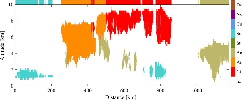
A. Guillaume et al.: Footprint-scale cloud type mixtures                                                                                 4367

Figure 4. Distribution of (a) minimum and (c) maximum length for 5 of the first 200 cloud scenes. The five scenes are, from top to bottom,
(Ac, Sc) in blue, (As, Sc, Cu) in orange, (Ci, As, Cu, Dc) in yellow, (As, Ac, Ns, Dc) in purple, and (Ci, As, Ac, St, Sc) in green, and their
respective ranks are 1, 26, 51, 76, and 101. In panels (b) and (d), the number of scenes were obtained by summing the number of scenes
present a different lengths.

Figure 5. Cloud type vertical cross section defined by the values of the cloud_scenario variables of the 2B-CLDCLASS product. Each color
corresponds to a different cloud type (legend on right). Color segments on top of the figure indicate the horizontal extent of a cloud measured
at its top.

   To illustrate the effects of these opposing behaviors, we              of four CloudSat profiles with this particular scene, with
consider the scene (As, Sc, Cu) length distribution. Since                three possible length combinations: (1 + 1 + 2), (1 + 2 + 1),
the minimum length of all cloud distributions in Fig. 6 is                or (2 + 1 + 1). The frequency of each individual cloud type,
one CloudSat profile, there is only one possible cloud length             As, Sc, or Cu, is smaller at the scale of four CloudSat pro-
combination (1 + 1 + 1) that will sum to the minimum pos-                 files than it is at a length of three CloudSat profiles in Fig. 6.
sible length of the scene (As, Sc, Cu). This is indeed the                However, there are more (As, Sc, Cu) scenes at length 4 than
value observed on the far left of each red-orange curve                   at 3 in Fig. 4a and c. This indicates that the increase in possi-
in Fig. 4a and c. Next, consider a measurement consisting                 ble combinations is more important than the individual cloud

www.atmos-meas-tech.net/12/4361/2019/                                                        Atmos. Meas. Tech., 12, 4361–4377, 2019
4368                                                                  A. Guillaume et al.: Footprint-scale cloud type mixtures

Figure 6. Horizontal cloud chord length frequency histograms for each of the eight CloudSat cloud types and clear sky. The cloud chord
length was obtained at the cloud top (see Fig. 5) unlike that obtained in Guillaume et al. (2018).

frequency decrease for larger scales. This reasoning applies         of all observed scenes. A total of 41.5 % of AIRS FOVs
for increasing lengths until the decreasing frequency of indi-       are completely cloudy while 27.8 % are partly cloudy ac-
vidual cloud types between two consecutive lengths is more           cording to 2B-CLDCLASS. Below the differences in cloud-
important. There are very few single As, Sc, or Cu clouds            thermodynamic-phase detection and ice cloud property re-
observed at large lengths (far right scale of Fig. 6) resulting      trievals are quantified for the types of scenes summarized in
in a very small number of observed (As, Sc, Cu) scenes in            Table 2.
Fig. 4a and c, despite the large number of length combina-
tion possibilities that may contribute.                              4.2   Cloud thermodynamic phase

                                                                     The occurrence frequency histogram of the sum of all
4     Cloud scene dependence of AIRS cloud properties
                                                                     thermodynamic-phase tests is shown for cloudy sky with one
We will now establish differences in the AIRS                        cloud type in Fig. 7. Homogeneous cloud scenes serve as an
thermodynamic-phase and ice cloud properties in the                  ideal point of reference for establishing cloud-phase sensitiv-
presence of complex and simple cloud types using coinci-             ity benchmarks. Overall, there is strong differentiation in the
dent cloud scenes. In this section, the scenes are determined        cloud thermodynamic phase among cloud scenes with sin-
at the AIRS FOV resolution (approximately 15 km). We                 gle cloud types. Ice tests dominate Ci, Ns, Dc, and As, while
briefly summarize general categories of cloud scene statistics       liquid and undetermined tests dominate Ac, Sc, and Cu.
in Sect. 4.1. The AIRS cloud-thermodynamic-phase tests                  The ice tests dominate the Ci cloud scenes and reaffirm the
are discussed separately for single and mixed cloud scenes           sensitivity of AIRS to ice clouds. CloudSat-classified clear
in Sect. 4.2. The AIRS ice cloud τi and rei , error estimates,       scenes contain occasional occurrences of AIRS-detected thin
averaging kernels (i.e., information content), and χ 2 residual      cirrus (+1 and +2), consistent with either thin cirrus that
fits between observed and simulated radiances are shown in           is undetected by the CloudSat radar or thicker cirrus within
Sect. 4.3.                                                           the AIRS footprint but to the side of the CloudSat ground
                                                                     track (e.g., Kahn et al., 2008). A few occurrences of −1 and
4.1    Types of cloud scenes                                         −2 may also arise from spatial mismatches between AIRS
                                                                     and CloudSat scenes, or from stratus below 1 km in alti-
Table 2 summarizes five types of scenes at the 15 km AIRS            tude that is undetected by CloudSat. In the Sc cloud scenes,
FOV scale: (i) clear sky, (ii) cloudy sky with one cloud type,       trade cumulus clouds dominate as previously shown by Yue
(iii) partly cloudy sky with one cloud type, (iv), cloudy sky        et al. (2011) and Kahn et al. (2017). A larger proportion of
with multiple cloud types, and (v) partly cloudy sky with            liquid tests, and a smaller proportion of ice tests, is observed
multiple cloud types. The raw counts and the relative per-           in the Sc cloud scenes compared to clear sky, but undeter-
centages for the 2-year observing period are shown. The              mined phase is dominant in both scene types. The Cu and Sc
dominance of clear sky (30.7 %) at 15 km is apparent and             cloud scene histograms are generally similar with more un-
is consistent with an absence of thin cloud features in the          determined cases for Cu, but with a slight reduction of liquid
2B-CLDCLASS data set. Cloudy sky scenes with one cloud               and slight increase in ice observed for Cu compared to Sc.
type (multiple cloud types) amount to 31.3 % (10.2 %) of all            The As cloud scene histogram in Fig. 7 is overwhelmingly
observed scenes, while partly cloudy sky scenes with one             dominated by ice. The undetermined cases in part may re-
cloud type (multiple cloud types) amount to 23.5 % (4.3 %)           sult from supercooled liquid or mixed-phase clouds that po-

Atmos. Meas. Tech., 12, 4361–4377, 2019                                                 www.atmos-meas-tech.net/12/4361/2019/
A. Guillaume et al.: Footprint-scale cloud type mixtures 4369
Table 1. Horizontal cloud chord length median and median absolute deviation for each cloud type (km).
Cloud type nc Ci As Ac St Sc Cu Ns Dc
Median 6.6 8.8 12.1 1.1 3.3 1.1 1.1 15.4 14.3
Median absolute deviation 5.5 7.7 11.0 0.0 2.2 0.0 0.0 13.2 9.9
Figure 7. AIRS cloud_phase_3x3 histograms for cloudy sky with one cloud type (i.e., all CloudSat profiles have the same cloud type and
no clear sky). The red, green, and blue bars indicate liquid, undetermined, and ice phase, respectively. Each histogram sums to 1.0 and does
not show how many counts relative to another histogram. Relative counts could be inferred from the percentages listed in the second to left
column of Table 3.
tentially could be distinguished with an improved phase al- nate in the Dc cloud scene histogram although a very small
gorithm that factors in the spectral midinfrared signature of proportion of −1, 0, and +1 occur. Inspection of AIRS gran-
supercooled liquid (e.g., Rowe et al., 2013). The Ac and As ules (not shown) demonstrates that the spectral signatures
cloud scene histograms are very different from each other, used in thermal infrared phase tests break down in the pres-
with a majority of undetermined and liquid for Ac and a ence of overshooting convection and other ice clouds within
majority of ice for As, consistent with aircraft observations a few Kelvin of the tropopause (e.g., Kahn et al., 2018).
(Mazin, 2006). The preponderance of undetermined phase The occurrence frequencies of cloud phase for partly
for Ac may indicate frequent supercooled liquid cloud tops cloudy sky with one cloud type are shown in Fig. 8. The
(Zhang et al., 2010). Ham et al. (2013) showed that Ac are biggest change is the relative ordering of the ranks among
typically 2–3 km lower in altitude than As, and this proba- cloud scene types between Figs. 7 and 8. Ac is now more
bly explains some of the difference in liquid and ice phase, common than As, as horizontal extent and frequency both
as lower clouds are usually warmer. The Ns cloud scene his- explain reordering of rankings in Figs. 7 and 8 (Miller et al.,
togram is dominated by ice detection with occasional liquid 2014; Guillaume et al., 2018). There are more subtle changes
and undetermined cloud tops. The Ns cloud scene also has in the cloud-phase histograms that are consistent with partly
significant height overlap with Ac and As, with most tops for cloudy sky. A weaker spectral signature for partly cloudy
all three types typically located below 9 km. Ice tests domi- scenes results in slightly greater counts of unknown phase
www.atmos-meas-tech.net/12/4361/2019/ Atmos. Meas. Tech., 12, 4361–4377, 20194370 A. Guillaume et al.: Footprint-scale cloud type mixtures
Figure 8. AIRS cloud_phase_3x3 histograms for partly cloudy sky with one cloud type. All else equal to Fig. 7.
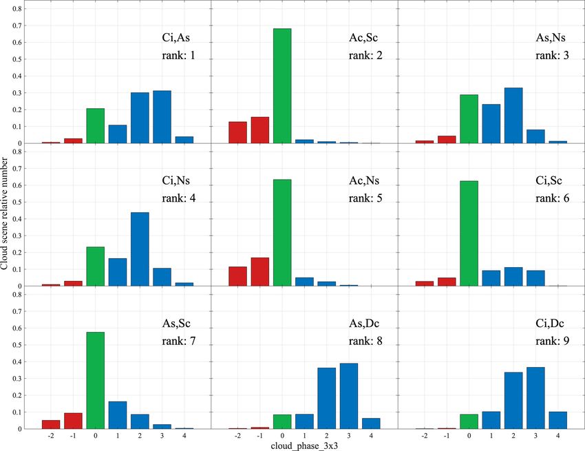
Table 2. Total counts and relative percentages of five cloud scene Sc with undetermined phase the most frequent. (Ci, Sc) is
categories at the AIRS FOV scale: clear sky, cloudy sky with one a common cloud scene in the low latitudes as trade cumu-
cloud type, partly cloudy sky with one cloud type, cloudy sky with lus (Sc cloud type) and is frequently found under thin cirrus
multiple cloud types, and partly cloudy sky with multiple cloud (Chang and Li, 2005). Furthermore, the spectral signatures of
types. the two types of clouds frequently cancel, giving an undeter-
mined phase result in the spectral tests used here (not shown).
Type of scene Total count percent The (Ci, As) cloud scene shows a slight reduction in liquid
Clear 7 175 523 30.7 detections and a slight increase in ice detections compared to
Cloudy sky with one cloud type 7 332 076 31.3 As alone. While the As cloud scene in Fig. 7 is dominated
Partly cloudy sky with one cloud type 5 506 074 23.5 by +2, the (Ci, As) cloud scene is dominated by +2 and +3.
Cloudy sky with multiple cloud types 2 377 259 10.2 This suggests that a mixture of Ci and As together can trigger
Partly cloudy sky with multiple 1 008 158 4.3 more ice tests in AIRS than As alone.
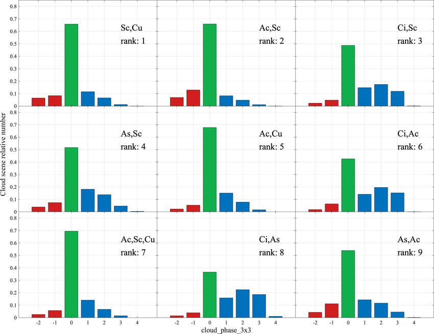
cloud types The nine most frequent partly cloudy scenes with multi-
All 23 399 090 100.00 ple cloud types are shown in Fig. 10. As with the differences
between Figs. 7 and 8, the biggest change is the relative or-
dering of the ranks among cloud scene types between Figs. 9
and 10. Furthermore, there are additional (yet subtle) changes
and also subtle shifts in liquid- and ice-phase tests in Fig. 8 in the phase test histograms for the cloud scenes that are com-
compared to Fig. 7. In the Ac cloud scene histograms, there mon between Figs. 9 and 10.
is a small but discernible increase in ice tests in Fig. 8 com- In most mixed cloud scenes in both Figs. 9 and 10, the
pared to Fig. 7. Horizontally heterogeneous Ac appears to characteristics of the histograms are similar either to single
have more frequent ice detection than horizontally homoge- types or have combined characteristics of the multiple cloud
neous Ac. types contained within the cloud scene. These results are en-
The nine most frequent cloudy scenes with multiple cloud couraging and reaffirm the capabilities of thermal-infrared
types are shown in Fig. 9. The (Ci, Sc) cloud scene ice- cloud-phase determination (Jin and Nasiri, 2014) and exhibit
phase histogram resembles a hybrid of histograms for Ci and
Atmos. Meas. Tech., 12, 4361–4377, 2019 www.atmos-meas-tech.net/12/4361/2019/A. Guillaume et al.: Footprint-scale cloud type mixtures 4371
Figure 9. AIRS cloud_phase_3x3 histograms for cloudy sky with multiple cloud types for the top nine ranked cloud scenes in order of
occurrence frequency.
consistency with cloud types from the CloudSat radar. We robust retrievals within cloud scenes that are dominated by
note, however, that the AIRS phase determination has some ice phase in the histograms (Fig. 7).
ambiguity in overlapping ice and liquid cloud layers as pre- The Ci cloud scene has mean values of τi = 1.91 and
viously shown by Jin and Nasiri (2014). rei = 25.4 µm; an AK = 1.0, the highest of any scene type;
and lower errors compared to other types in Table 3. The As
4.3 Ice cloud properties cloud scene has a larger mean of τi = 2.42 compared to the
Ac cloud scene with a mean of τi = 1.65 (Table 3). Interest-
The mean ice cloud property retrievals are summarized in Ta- ingly, the mean value and error estimate of rei is lower for
ble 3 for cloudy sky with one cloud type only for the ice-only Ac than As, exhibiting differentiation between these two mi-
portions of the cloud-phase histograms depicted in Fig. 7. dlevel cloud types. However, a much smaller proportion of
Scenes identified as clear sky exhibit properties of a small Ac is ice compared to As (Fig. 7).
population of thin cirrus detected by AIRS (Fig. 7) with mean The Ns cloud scene in Table 3 contains larger mean val-
values of τi = 0.77 and rei = 20.9 µm (Table 3). The AKs are ues of τi than Ci and Ac cloud scenes, but these values are
notably lower and the relative error for τi is higher than other similar to those for As; however, the mean values are lower
cloud scenes. The Sc cloud scene shows a small population than Cu and Dc cloud scenes (Table 3). A lower value of τi is
of cirrus that go undetected in 2B-CLDCLASS (Fig. 7) and characteristic of diffuse cloud tops where the infrared emis-
have mean values of τi = 1.30 and rei = 20.6 µm (Table 3). sion may originate several kilometers deep within the cloud
The AKs are also lowest in Table 3 for Sc relative to other (e.g., see Kahn et al., 2008; Holz et al., 2006). The reduced
cloud scenes with similarly high errors in τi and rei . Kahn AK = 0.88 for the Ns cloud scenes illustrates that a diffuse
et al. (2008, 2015) have shown that AIRS is very sensitive cloud top is more problematic for ice cloud retrievals. Cu
to thin cirrus; thus some ice clouds in CloudSat-identified Sc cloud scenes with ice cloud tops occur a small amount of the
cloud scenes are expected. Because tenuous ice clouds have time (Fig. 7); furthermore, Cu is infrequent in CloudSat clas-
smaller values of τi and rei , the lower estimates of informa- sification (1.7 % of all clouds). The horizontal extent of Cu is
tion content and larger error estimates are promising. These also much smaller than Dc (see Table 1). Interestingly, τi is
tenuous ice cloud retrievals are differentiated well from more
www.atmos-meas-tech.net/12/4361/2019/ Atmos. Meas. Tech., 12, 4361–4377, 20194372 A. Guillaume et al.: Footprint-scale cloud type mixtures
Table 3. Cloud ice properties for cloudy sky with one cloud type (i.e., all CloudSat profiles have the same cloud type). Proportions and
relative errors are in percent. The effective radius is in micrometers (µm).
Cloud Cloudy Mean τi τi % Mean rei rei % χ2
type single τi relative averaging passing rei relative averaging passing residual
type error kernel QC for error kernel QC for fit
proportion τi rei
nc 49.5 0.77 14.88 0.71 75.09 20.9 5.6 0.97 34.1 3.3
As 14.0 2.42 6.41 0.92 97.36 24.5 4.7 0.98 79.9 2.9
Sc 11.5 1.30 15.12 0.69 82.63 20.6 6.5 0.96 48.6 3.2
Ci 11.3 1.91 2.21 0.99 96.44 25.4 2.6 1.00 74.2 4.0
Ns 8.6 2.41 8.70 0.88 98.11 23.6 5.6 0.98 87.0 2.4
Ac 2.9 1.65 6.66 0.91 93.45 22.1 4.1 0.98 59.0 4.1
Dc 1.7 5.47 3.53 0.98 98.64 27.1 7.1 0.96 71.9 3.2
Cu 0.6 2.92 5.99 0.94 94.37 26.5 6.1 0.97 70.6 3.9
St 0.001 2.33 15.37 0.63 100.00 27.3 4.9 0.98 70.0 4.1
Figure 10. AIRS cloud_phase_3x3 histograms for partly cloudy sky with multiple cloud types for the top nine ranked cloud scenes in order
of occurrence frequency.
larger for Cu cloud scenes than for all categories except Dc 2014; Kahn et al., 2018). These Cu cases are likely transient
cloud scenes (Table 2). cumulus congestus at altitudes cold enough for cloud top
The mean Cu value of rei = 26.5 µm is larger than most glaciation. The Dc cloud scene has the largest mean τi = 5.47
cloud scenes. This is consistent with larger ice particles ob- of all cloud scenes with a very dense cloud top that saturates
served at the tops of convection instead of small ice particles the infrared emission signal in contrast to Ns. The values of
in thin cirrus at the same cloud top temperature (e.g., Yuan rei for Dc are similar to Cu (Table 3), with a slight reduction
and Li, 2010; Protat et al., 2011; van Diedenhoven et al., in the rei AK = 0.96 and τi AK = 0.98 relative to Ci cloud
Atmos. Meas. Tech., 12, 4361–4377, 2019 www.atmos-meas-tech.net/12/4361/2019/A. Guillaume et al.: Footprint-scale cloud type mixtures 4373
Table 4. Cloud ice properties for partly cloudy sky with one cloud type. All else the same as Table 3.
Cloud Partly cloudy Mean τi τi % Mean rei rei % χ2
type single τi relative averaging passing rei relative averaging passing residual
type error kernel QC for error kernel QC for fit
proportion τi rei
Sc 74.79 0.93 14.45 0.71 73.91 21.2 5.7 0.97 36.8 3.5
Ci 10.44 0.71 3.69 0.96 87.98 22.5 2.8 0.99 62.0 4.2
Ac 5.08 0.94 5.95 0.92 88.41 20.8 3.6 0.99 52.6 4.6
As 4.83 1.09 14.40 0.72 90.47 19.9 6.4 0.96 46.5 3.1
Cu 4.80 0.87 12.78 0.76 74.49 21.1 5.2 0.97 38.2 3.7
Ns 0.05 1.69 14.50 0.71 85.08 22.9 7.1 0.96 45.3 3.7
Dc 0.01 4.63 3.44 0.98 93.58 26.8 6.4 0.96 53.8 3.9
St 0.01 0.79 8.95 0.88 84.00 21.3 6.3 0.96 64.0 3.9
scenes (Table 3). This is consistent with reduced sensitivity have small horizontal scales and are averaged with clear sky
for high values of τi (e.g., Huang et al., 2004). in an AIRS pixel. Mixed (Cu, Nc) cloud scenes are especially
The relative variations between the ice cloud retrieval problematic for plane-parallel radiative transfer calculations.
properties for cloudy sky with one cloud type in Ta- This results in more uncertain retrievals of ice cloud prop-
ble 3 are consistent with expectations of infrared sensitiv- erties for partial cloud (Cu, Nc) in Table 3 than those for the
ity. CloudSat-observed Ci cloud scenes have smaller error pure Cu cases in Table 2, which are more likely to completely
estimates and higher information content in comparison to fill an AIRS scene.
Sc, consistent with Sc scenes containing tenuous cirrus that The ice cloud property retrievals for cloud scenes that
goes undetected by 2B-CLDCLASS. Larger τi and rei are ob- contain multiple cloud types are summarized in Table 5 for
served at the tops of convective ice clouds such as Dc and Cu cloudy scenes and Table 6 for partly cloudy scenes. These ta-
compared to stratiform clouds such as As and Ci. Differences bles list the nine most frequent cloud scene types as depicted
in ice cloud properties between Ac and As cloud scenes are in Figs. 9 and 10. Four of the nine cloud scenes are com-
consistent with observed differences in scene heterogeneity mon between Tables 5 and 6. There is a general tendency
and cloud top height. for reductions of τi , increases in percent relative error, and
The mean ice cloud property retrievals are summarized slight reductions in AKs in Table 6 for the seven common
in Table 4 for partly cloudy sky with one cloud type with cloud scenes in Table 5. Changes in rei -related variables are
cloud-phase histograms depicted in Fig. 8. The biggest dif- smaller than changes in τi -related variables.
ference between Tables 3 and 4 is the relative frequency of To summarize Tables 3–6, larger differences in ice cloud
occurrence with large differences between cloud scenes with property retrievals are found between different cloud types
or without clear sky. Another significant change is an over- than between cloudy and partly cloudy scenes. However,
all reduction in AKs and magnitude of τi , with an increase the differences between cloud scene types are the sharpest
in χ 2 in Table 4, consistent with partly cloudy scenes. The for the subset of cloudy scenes with one cloud type (Ta-
changes in rei AKs, magnitudes, and error estimates between ble 3). The AIRS cloud property retrievals are not greatly
Tables 3 and 4 are smaller than those for τi . Overall, the dif- impacted by mixtures of cloud types within the AIRS foot-
ferences between Tables 3 and 4 are reassuring in that the print, and ice cloud property differences among cloud scenes
AIRS retrieval is responding to partly cloudy scenes by re- are broadly consistent with the expected performance of in-
ducing information content and the magnitude of τi , while frared retrievals among these cloud types.
χ 2 residuals are increasing somewhat.
The As and Ac cloud scenes in Table 4 are very similar
to As and Ac cloud scenes in Table 3 except for slight re- 5 Summary
ductions in τi and rei . Scenes in Table 4 are partly cloudy,
implying a weaker infrared cloud signal. The Ci cloud scene A method is described to classify cloud mixtures of cloud
in Table 4 shows slight reductions in τi and rei from the Ci top types, termed cloud scenes, using the 2B-CLDCLASS
cloud scene in Table 3. cloud type classification obtained from the 94 GHz Cloud-
The differences between Tables 3 and 4 are more signif- Sat radar. The scale dependence of the cloud scenes is quan-
icant for the convective ice clouds, however. The Cu cloud tified. The method is initially applied to 2 years of Cloud-
scene τi and AK are smaller while errors are larger in Table 4 Sat data collocated within the Atmospheric Infrared Sounder
compared to the pure Cu cloud scene in Table 3. This is ex- (AIRS)/Atmospheric Microwave Sounding Unit (AMSU)
pected as Cu clouds are several kilometers in depth but often field of regard (FOR) at a 45 km scale. Given the 45 km
www.atmos-meas-tech.net/12/4361/2019/ Atmos. Meas. Tech., 12, 4361–4377, 20194374 A. Guillaume et al.: Footprint-scale cloud type mixtures
Table 5. Cloud ice properties for cloudy sky with multiple cloud types for the first nine most observed cloud scenes at the AIRS FOV scale.
All else the same as Table 4.
Cloud Mixed Mean τi τi % Mean rei rei % χ2
scene scenes τi relative averaging passing rei relative averaging passing residual
proportion error kernel QC for error kernel QC for fit
τi rei
Ci,As 16.7 2.52 4.05 0.96 97.56 24.7 3.8 0.99 74.6 3.5
Ac,Sc 16.0 1.31 10.41 0.81 85.92 21.9 5.0 0.97 53.7 4.0
As,Ns 11.0 2.07 10.66 0.83 97.01 22.4 5.7 0.97 81.6 2.6
Ci,Ns 7.2 2.14 6.84 0.93 97.39 22.9 4.3 0.98 85.8 2.8
Ac,Ns 6.1 1.75 12.83 0.77 91.58 21.2 6.0 0.97 69.9 3.1
Ci,Sc 5.2 1.00 4.61 0.95 84.98 24.5 3.1 0.99 60.7 4.3
As,Sc 4.8 1.34 16.31 0.66 91.55 19.7 6.6 0.96 57.0 2.9
As,Dc 3.7 5.22 3.12 0.99 99.07 28.0 6.8 0.96 65.8 3.5
Ci,Dc 3.4 4.30 2.82 0.99 98.61 27.4 4.9 0.98 62.0 4.1
Table 6. Cloud ice properties for partly cloudy sky with multiple cloud types for the first nine most observed cloud scenes at the AIRS FOV
scale. All else the same as Table 5.
Cloud Mixed Mean τi τi % Mean rei rei % χ2
scene scenes τi relative averaging passing rei relative averaging passing residual
proportion error kernel QC for error kernel QC for fit
τi rei
Sc,Cu 18.0 1.03 14.00 0.73 76.20 21.8 5.9 0.97 39.1 3.7
Ac,Sc 20.1 0.87 6.34 0.92 84.99 21.4 4.0 0.98 54.9 4.4
Ci,Sc 17.8 0.70 4.07 0.95 86.31 22.6 2.9 0.99 61.1 4.2
As,Sc 5.2 1.16 14.36 0.72 88.08 20.4 6.3 0.96 47.9 3.4
Ac,Cu 3.4 0.94 4.84 0.95 86.14 23.0 4.1 0.98 56.3 4.7
Ci,Ac 3.3 1.18 2.93 0.98 93.16 22.3 2.5 0.99 56.4 5.0
Ac,Sc,Cu 3.2 0.83 5.36 0.94 85.47 22.7 4.3 0.98 59.5 4.4
Ci,As 2.7 1.22 7.10 0.89 92.41 21.3 4.2 0.98 52.5 3.9
As,Ac 2.1 1.14 8.07 0.87 90.54 21.3 4.5 0.98 48.6 4.3
scale and approximately 50 coinciding CloudSat profiles, The cloud scenes are organized into five categories:
each with 125 levels, the total number of possible scenes (i) clear sky, (ii) cloudy sky with one cloud type, (iii) partly
within an AMSU FOR is 950×125 . This very large number of cloudy sky with one cloud type, (iv), cloudy sky with multi-
possible scenes is reduced to 256 by making three assump- ple cloud types, and (v) partly cloudy sky with multiple cloud
tions in the classification. First, only the cloud type at the types. Summarizing AIRS cloud top property retrievals for
cloud top is considered. Second, the occurrence frequency of cloudy sky with one cloud type, there is strong differentiation
each cloud type within the cloud scene is disregarded; thus, in the cloud thermodynamic phase. Ice phase dominates Ci,
there is no consideration of the counts of each cloud type. Ns, Dc, and As, while liquid and undetermined phase domi-
Third, the sequence of cloud types along the orbit segment is nate Ac, Sc, and Cu. The results are similar for partly cloudy
not considered. These three assumptions make mixed cloud sky with one cloud type with an increase in unknown cloud
scene classification tractable and are broadly consistent with phase and χ 2 residuals, as well as a reduction in informa-
the sensitivity of infrared sounders to clouds. They are also tion content for some cloud types. A similar set of calcula-
independent of the spatial scale of a scene and therefore can tions were performed for both cloudy and partly cloudy skies
be generalized to all horizontal scales. A total of 210 out of with multiple cloud types. In most cloud scenes with multi-
256 possible cloud scenes are observed in a 2-year period ple cloud types, the changes in the ice properties are gener-
from 1 July 2006 to 30 June 2008. The maximum number ally either small or reflect the combined characteristics of the
of cloud scenes occurs at a horizontal scale of 105 km with multiple cloud types contained within the cloud scene. The
fewer cloud scenes at larger and smaller scales, and the ma- sensitivity of thermal infrared cloud-phase determination is
jority of observed cloud scenes contain single cloud types. consistent with independently determined cloud typing from
the CloudSat radar for clouds detected by CloudSat.
Atmos. Meas. Tech., 12, 4361–4377, 2019 www.atmos-meas-tech.net/12/4361/2019/A. Guillaume et al.: Footprint-scale cloud type mixtures 4375
The relative magnitude of differences in rei and τi , and Author contributions. AG designed and implemented the cloud
their averaging kernels (AKs) and error estimates, and the scene classification scheme as well as the cloud scene and cloud
χ 2 residual between simulated and observed radiances are type scale dependence studies. BK designed and AG implemented
consistent with expectations of infrared retrieval sensitivity the study of AIRS thermodynamic-phase and ice cloud properties as
to different cloud types. Smaller error estimates and higher a function of cloud scenes and types. GM designed, implemented,
and generated the AIRS/AMSU/CloudSat matchup product. GM,
information content (AKs) within Ci cloud scenes are ob-
BW, and HH designed the data system that generated this product.
served in comparison to thin cirrus likely missed by Cloud- AG and BK prepared the manuscript with contributions from all
Sat in clear sky and Sc scenes. Larger τi and rei are observed coauthors.
at the tops of convective ice clouds. Differences in retrieved
cloud properties between Ac and As cloud scenes are consis-
tent with differences in their scene heterogeneity and cloud Competing interests. The authors declare that they have no conflict
temperature. Variations in ice cloud property retrievals are of interest.
larger between types of cloud scenes than between cloudy
and partly cloudy/mixed cloud scenes.
The fidelity of AIRS-retrieved cloud-phase and ice cloud Acknowledgements. Part of this research was carried out at the Jet
microphysics was tested within scenes with both uniform Propulsion Laboratory (JPL), California Institute of Technology,
and nonuniform cloud cover, as well as one or more cloud under a contract with the National Aeronautics and Space Adminis-
types within the scene. As with phase, retrieval differences tration. The authors thank two reviewers for helpful and insightful
are shown to be larger among cloud types rather than be- comments that led to an improved manuscript. This project was sup-
tween uniform and mixed cloud scenes. ported by NASA’s Making Earth Science Data Records for Use in
Research Environments (MEaSUREs) program.
New methodologies for simultaneous retrievals of cloud
microphysical properties and temperature and specific hu-
midity profiles that include clouds in the forward radiative
Financial support. This research has been supported by NASA
transfer (e.g., De Souza-Machado et al., 2018; Irion et al., (grant no. NNH17ZDA001N).
2018) necessitate careful investigation of the effects of cloud
mixtures on retrieved cloud properties. The bias and root-
mean square error of AIRS temperature and specific humid- Review statement. This paper was edited by Alexander
ity soundings depend on cloud type (Yue et al., 2013; Wong Kokhanovsky and reviewed by two anonymous referees.
et al., 2015). A more rigorous evaluation of scene complex-
ity is necessary for optimizing the retrieval configuration of
future sounding algorithms (Irion et al., 2018) and for vali-
dating their products.
This investigation shows that careful inspection of References
footprint-scale AIRS cloud property retrievals is consistent
with expectations of infrared sensitivity to different cloud Barnes, E. A. and Polvani, L.: Response of the Midlatitude Jets,
types defined with the 94 GHz CloudSat radar. Other cloud and of Their Variability, to Increased Greenhouse Gases in the
observations, such as MODIS, may be used in a similar anal- CMIP5 Models, J. Climate, 26, 7117–7135, 2013.
Bony, S., Colman, R., Kattsov, V. M., Allan, R. P., Bretherton, C. S.,
ysis to the one described here. MODIS captures the off-
Dufresne, J.-L., Hall, A., Hallegatte, S., Holland, M. M., Ingram,
nadir portion of the AIRS swath and the fine-scale variability
W., Randall, D. A., Soden, B. J., Tselioudis, G., and Webb, M.
within AIRS footprints. Wang et al. (2016) used the cloud J.: How Well Do We Understand and Evaluate Climate Change
typing in CloudSat to cross validate with cloud typing using Feedback Processes?, J. Climate, 19, 3445–3482, 2006.
MODIS-defined cloud types. This establishes a link between Ceppi, P., Hartmann, D. L., and Webb, M. J.: Mechanisms of the
cloud types obtained from CloudSat and MODIS. A rigor- Negative Shortwave Cloud Feedback in Middle to High Lati-
ous estimation of the pixel-scale relationships between cloud tudes, J. Climate, 29, 139–157, 2016.
properties obtained from CloudSat, MODIS, and AMSU will Chahine, M. T., Pagano, T. S., Aumann, H. H., Atlas, R., Barnet,
help to further advance multisensor and multivariate geo- C., Blaisdell, J., Chen, L., Divakarla, M., Fetzer, E. J., Goldberg,
physical retrievals (e.g., Irion et al., 2018). M., Gautier, C., Granger, S., Hannon, S., Irion, F. W., Kakar,
R., Kalnay, E., Lambrigtsen, B. H., Lee, S., Le Marshall, J.,
Mcmillan, W. W., Mcmillin, L., Olsen, E. T., Revercomb, H.,
Rosenkranz, P., Smith, W. L., Staelin, D., Strow, L. L., Susskind,
Data availability. CloudSat data were obtained through the Cloud-
J., Tobin, D., Wolf, W., and Zhou, L.: The Atmospheric Infrared
Sat Data Processing Center (http://www.cloudsat.cira.colostate.
Sounder (AIRS): Improving weather forecasting and providing
edu/, Cooperative Institute, 2019). The combined data files used in
new insights into climate, B. Am. Meteorol. Soc., 87, 911–926,
this work are available at the Goddard Earth Sciences Data and In-
https://doi.org/10.1175/BAMS-87-7-911, 2006.
formation Services Center (Fetzer at al., 2013).
Chang, F. L. and Li, Z.: A near global climatology of single-layer
and overlapped clouds and their optical properties retrieved from
www.atmos-meas-tech.net/12/4361/2019/ Atmos. Meas. Tech., 12, 4361–4377, 2019You can also read