Three-dimensional radiative transfer effects on airborne and ground-based trace gas remote sensing - DORA 4RI
←
→
Page content transcription
If your browser does not render page correctly, please read the page content below
Atmos. Meas. Tech., 13, 4277–4293, 2020
https://doi.org/10.5194/amt-13-4277-2020
© Author(s) 2020. This work is distributed under
the Creative Commons Attribution 4.0 License.

Three-dimensional radiative transfer effects on airborne and
ground-based trace gas remote sensing
Marc Schwaerzel1,2 , Claudia Emde3 , Dominik Brunner1 , Randulph Morales1 , Thomas Wagner4 , Alexis Berne2 ,
Brigitte Buchmann1 , and Gerrit Kuhlmann1
1 Empa,   Swiss Federal Laboratories for Materials Science and Technology, Dübendorf, Switzerland
2 Environmental  Remote Sensing Laboratory, École Polytechnique Fédérale de Lausanne, Lausanne, Switzerland
3 Meteorological Institute, Ludwig Maximillian University, Munich, Germany
4 Satellite Remote Sensing Group, Max Planck Institute for Chemistry, Mainz, Germany

Correspondence: Gerrit Kuhlmann (gerrit.kuhlmann@empa.ch)

Received: 16 April 2020 – Discussion started: 4 May 2020
Revised: 7 July 2020 – Accepted: 15 July 2020 – Published: 14 August 2020

Abstract. Air mass factors (AMFs) are used in passive               borne imaging spectrometer observing the NO2 plume emit-
trace gas remote sensing for converting slant column den-           ted from a tall stack. The plume was imaged under different
sities (SCDs) to vertical column densities (VCDs). AMFs             solar zenith angles and solar azimuth angles. To demonstrate
are traditionally computed with 1D radiative transfer mod-          the limitations of classical 1D-layer AMFs, VCDs were then
els assuming horizontally homogeneous conditions. How-              computed assuming horizontal homogeneity. As a result, the
ever, when observations are made with high spatial resolu-          imaged NO2 plume was shifted in space, which led to a
tion in a heterogeneous atmosphere or above a heterogeneous         strong underestimation of the total VCDs in the plume max-
surface, 3D effects may not be negligible. To study the im-         imum and an underestimation of the integrated line densities
portance of 3D effects on AMFs for different types of trace         that can be used for estimating emissions from NO2 images.
gas remote sensing, we implemented 1D-layer and 3D-box              The two examples demonstrate the importance of 3D effects
AMFs into the Monte carlo code for the phYSically cor-              for several types of ground-based and airborne remote sens-
rect Tracing of photons In Cloudy atmospheres (MYSTIC),             ing when the atmosphere cannot be assumed to be horizon-
a solver of the libRadtran radiative transfer model (RTM).          tally homogeneous, which is typically the case in the vicinity
The 3D-box AMF implementation is fully consistent with              of emission sources or in cities.
1D-layer AMFs under horizontally homogeneous conditions
and agrees very well ( < 5 % relative error) with 1D-layer
AMFs computed by other RTMs for a wide range of sce-
narios. The 3D-box AMFs make it possible to visualize the           1   Introduction
3D spatial distribution of the sensitivity of a trace gas obser-
vation, which we demonstrate with two examples. First, we           Ground-based, space-based and airborne remote sensing of
computed 3D-box AMFs for ground-based multi-axis spec-              air pollutants and greenhouse gases from scattered sun-
trometer (MAX-DOAS) observations for different viewing              light are increasingly used for air pollutant monitoring (e.g.,
geometry and aerosol scenarios. The results illustrate how          Frankenberg et al., 2005; Richter et al., 2004; McPeters et al.,
the sensitivity reduces with distance from the instrument and       2015; Burrows et al., 1999; Zhou et al., 2012; Nowlan et al.,
that a non-negligible part of the signal originates from out-       2016) and for source detection and emission estimation (e.g.,
side the line of sight. Such information is invaluable for inter-   Mijling et al., 2013; Martin et al., 2003; Russell et al., 2012;
preting MAX-DOAS observations in heterogeneous environ-             Krueger et al., 1995). The most commonly applied trace gas
ments such as urban areas. Second, 3D-box AMFs were used            retrieval method in the ultraviolet, visible and near-infrared
to generate synthetic nitrogen dioxide (NO2 ) SCDs for an air-      spectral range is differential optical absorption spectroscopy
                                                                    (DOAS) (Platt and Stutz, 2008), which fits absorption cross

Published by Copernicus Publications on behalf of the European Geosciences Union.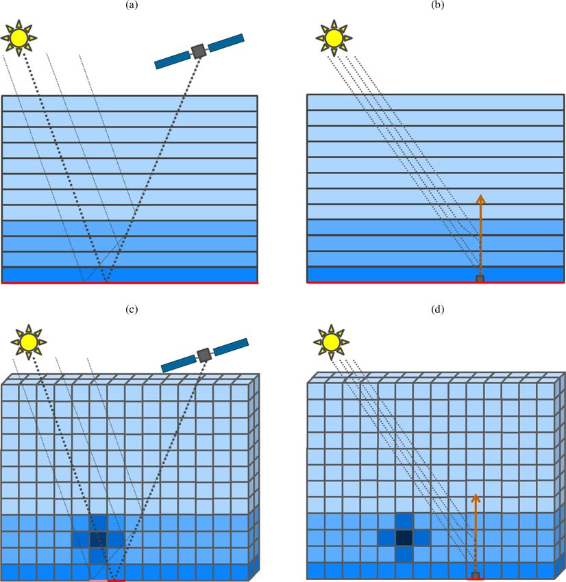
4278                       M. Schwaerzel et al.: Three-dimensional radiative transfer effects on trace gas remote sensing

sections of a trace gas to the measured spectra. The result of    the radiative transfer equation (Deutschmann et al., 2011).
the DOAS analysis is a slant column density (SCD), which is       In this study, we implemented both 1D-layer and 3D-box
the integrated trace gas concentration along the optical path     AMFs in the MYSTIC solver of the libRadtran RTM (Mayer
of the sunlight scattered towards the spectrometer. The opti-     and Kylling, 2005; Emde et al., 2016). The implementation
cal path depends on the illumination and viewing geometry,        was evaluated against the results of a RTM comparison study
on absorption and scattering by air molecules, aerosols and       (Wagner et al., 2007). Finally, the advantage and necessity of
clouds, and surface reflectance.                                  using 3D-box AMFs is demonstrated for a range of realistic
   A physically more meaningful quantity that is indepen-         ground-based and airborne remote sensing scenarios.
dent of the measurement geometry is the vertical column
density (VCD), which is the integrated trace gas concentra-
tion from the ground to the top of the atmosphere. The ra-        2     Methods
tio between SCD and VCD is called air mass factor (AMF)
                                                                  2.1    Air mass factors
(Solomon et al., 1987), which can be computed with a ra-
diative transfer model (RTM). To account for the vertical         Atmospheric trace gases can be measured with ground-,
variability in atmospheric properties, AMFs are computed          aircraft- and space-based spectrometers that measure solar ir-
for discrete vertical layers (layer AMFs) assuming horizon-       radiance scattered into the line of sight of the instrument (see
tal homogeneity (Palmer et al., 2001; Wagner et al., 2007;        Fig. 1). In the case of aircraft- and space-based observations,
Rozanov and Rozanov, 2010). In the past decades, numer-           a large fraction of the measured photons usually travels along
ous RTMs have been developed with the possibility to cal-         a main path (thick dashed line) representing a single reflec-
culate one-dimensional layer AMFs (e.g., Berk et al., 1999;       tion at the surface. In the case of ground-based observations,
Postylyakov, 2004; Rozanov et al., 2005; Wagner et al.,           the measured photons must follow a path with at least a single
2007; Spurr et al., 2001; Iwabuchi, 2006; Iwabuchi and            atmospheric scattering into the line of sight of the instrument
Okamura, 2017). The computation of layer AMFs is im-              (except for direct sun observations). Atmospheric scattering
plemented in most trace gas retrieval algorithms for satel-       and absorption is determined by the distribution and proper-
lite and ground-based observations applied today (Boersma         ties of molecules, aerosols and clouds, and it depends on the
et al., 2011; Irie et al., 2011; Wenig et al., 2008; Wu et al.,   wavelength of the radiation. Molecular scattering is particu-
2013). An alternative method is direct fitting, which is used     larly important in the UV range of the spectrum. Photons are
in few algorithms (e.g., Lerot et al., 2010).                     absorbed by the trace gases along the optical path from the
   Layer AMFs assume horizontal homogeneity, which is not         sun to the instrument. For a weak absorber such as NO2 , the
valid when the parameters affecting scattering and absorp-        abundance of the trace gas along the mean optical path can
tion along the path of the photons vary also horizontally,        be obtained by fitting an absorption cross section to the mea-
for example, in limb geometry near the polar vortex (Puk, ı̄te    sured spectrum. Thereby, the mean optical path is the total
et al., 2010) or in the presence of clouds (Mayer and Kylling,    length of all individual photon paths divided by the number
2005). Horizontal homogeneity is usually a valid assumption       of photons collected by the instrument. The result of the fit is
in coarse-resolution trace gas remote sensing from satellites,    a SCD, which is defined as
where small-scale horizontal variability is averaged over a                 Z
large pixel size. It is, however, often not valid for ground-     SCD =        c(l)dl,                                         (1)
based or airborne trace gas remote sensing at high resolution
                                                                           path
in polluted environments such as cities (e.g., Hendrick et al.,
2014; Popp et al., 2012; Schönhardt et al., 2015; Tack et al.,    with trace gas concentration c and optical path l. SCDs are
2017). This is particularly true for nitrogen dioxide (NO2 ),     not an intrinsic property of the atmosphere, since they de-
which has high spatial and temporal variability due to its        pend on the illumination and viewing geometry. Therefore,
short lifetime (Schaub et al., 2007). Other parameters affect-    for most applications, the main quantity of interest is the
ing the path of the measured photons like surface reflectance     VCD. It is defined as
and aerosol distributions may also have high spatial variabil-              TOA
                                                                            Z
ity in cities.
                                                                  VCD =           c(z)dz,                                     (2)
   To account for horizontal inhomogeneity, one-dimensional
(1D) layer AMFs need to be extended to three-dimensional                    z0
(3D) box AMFs. Notice that in previous studies (e.g.,             with surface elevation z0 and top of the atmosphere, TOA.
Rozanov and Rozanov, 2010) 1D-layer AMFs were some-               AMFs, defined as
times referred to as box AMFs. In this study, we will use the
                                                                            SCD
terms 1D-layer and 3D-box AMFs to clearly distinguish be-         AMF =         ,                                             (3)
tween them. The 3D-box AMFs can be implemented most                         VCD
easily in radiative transfer models that compute the paths        can be computed for a vertically varying atmosphere by di-
of many photons using a Monte Carlo approach to solve             viding the atmosphere in layers with uniform properties (see

Atmos. Meas. Tech., 13, 4277–4293, 2020                                              https://doi.org/10.5194/amt-13-4277-2020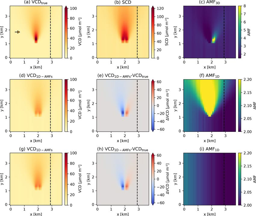
M. Schwaerzel et al.: Three-dimensional radiative transfer effects on trace gas remote sensing                              4279

Fig. 1a and b). The total AMF is then computed from the              SCDs, VCDs and AMFs can be computed for the whole
individual layer AMFs as                                          atmosphere, for individual vertical layers or for individual
         Pnz                                                      3D boxes. For the general case of an atmospheric box i with
               AMFk VCDk                                          constant concentration and optical properties, the AMF can
AMF = k=1    Pnz           ,                        (4)
               k=1 VCDk                                           be written as
                                                                                        R              R
with AMFk and VCDk being the AMF and VCD in the kth                          SCDi         path ci dl     path dl  Li
layer, respectively. The total AMF is thus a function not only    AMFi =              = R zi+1       =           = ,           (6)
                                                                             VCDi        zi ci dz
                                                                                                          h i     hi
of the atmospheric properties in each layer but also of the
shape of the vertical profile of the trace gas (Palmer et al.,                  R
                                                                  where Li = path dl is the mean optical path within the box of
2001).                                                            all photons that reach the instrument and hi is the height of
   Similarly, the atmosphere can be divided into boxes in all     the box. Since the 3D-box/1D-layer AMFs are usually simu-
three dimensions (i, j, k) with homogeneous optical proper-       lated for a sensor at a specific location in a three-dimensional
ties for each box (see Fig. 1c and d). The total AMF can be       model domain, the photons are traced backwards from the
computed from the 3D-box AMFs AMFi,j,k as                         sensor towards the sun to increase computational efficiency
          Pnx Pny Pnz                                             as described in Marchuk et al. (1980) and Emde and Mayer
            i=1 j =1 k=1 AMFi,j,k VCDi,j,k                        (2007). In addition, the commonly used variance reduction
AMF =                 Pn z                     ,           (5)
                         k=1 VCDk                                 method, known as “local estimate”, is applied at each scatter-
                                                                  ing event (Marshak and Davis, 2005). The method computes
where the denominator is a sum over VCDs in k different
                                                                  the probability of an individual photon to be scattered into
vertical layers that could, for example, be taken at the loca-
                                                                  the direction of the sun that is assigned as a weight wn to the
tion of an instrument or above the ground pixel of an aircraft-
                                                                  photon. The weights of all photons can be summed up to ob-
or space-based instrument. In this case, the AMF can be in-
                                                                  tain the radiance at the sensor. When a photon is scattered, a
terpreted as the instrument sensitivity to the trace gas under
                                                                  weighted photon path length (wn ·li ) is also calculated, where
investigation for measuring that specific VCD.
                                                                  li are the path lengths in each individual box i traversed by
2.2   Implementation of AMFs in MYSTIC                            the photon before the scattering event. The mean optical path
                                                                  within a box i is then obtained by summing up the weighted
The libRadtran RTM (available at http://www.libradtran.org,       photon path lengths of all photons as follows:
last access: 12 August 2020) can be used to calculate basic              PN
radiative quantities with different numerical solvers (Mayer                n wn li,n
                                                                  Li = P      N
                                                                                      ,                                        (7)
and Kylling, 2005; Emde et al., 2016). One of its solvers is                  n wn
MYSTIC, which uses the Monte Carlo technique to trace in-
dividual photons on their way from the source (e.g., sun) to      where N is the total number of photons. Li is then divided
the target (e.g., measurement instrument). Scattering, absorp-    by the height of the box/layer to obtain the 3D-box/1D-layer
tion and reflection processes are treated as random decisions     AMF.
with respective probability distributions. MYSTIC calculates
radiative quantities (irradiance, actinic flux at levels, radi-   3     Validation of the AMF modules
ance, absorption, emission, actinic flux, photon’s path length
and air mass factors) in 1D or 3D domains in spherical geom-      3.1    Evaluation scenarios
etry or in plane-parallel geometry (Emde and Mayer, 2007;
Emde et al., 2017). The 1D-layer and 3D-box AMFs were             The implementation of the 1D-layer and 3D-box AMF mod-
implemented following the same methodology as in McAr-            ule in MYSTIC was evaluated against the results of differ-
tim, which to our knowledge is the only other existing RTM        ent RTMs presented in an extensive RTM comparison study
capable of computing 3D-box AMFs (Deutschmann et al.,             (Wagner et al., 2007). The simulated scenarios are represen-
2011; Richter et al., 2013). Note that McArtim is no longer       tative for ground-based Multi-Axis-DOAS (MAX-DOAS)
actively developed.                                               measurements of scattered sunlight spectra for different el-
   AMFs depend on absorption and scattering processes af-         evation angles (see Fig. 1b and d for the case of zenith-sky
fecting the light path in the atmosphere. AMFs can be readily     observations). The nine models included four models using
calculated from the photon paths simulated by a Monte Carlo       full spherical geometry, four models using spherical geom-
radiative transfer model. The Monte Carlo technique traces        etry only for a subset of interactions and one model using
the paths of individual photons by describing the effects of      plane-parallel geometry. The 1D-layer AMFs computed by
absorption, scattering and reflection as random events with       these models agreed very well with differences mostly be-
specific probabilities (Mayer, 2009). To obtain a robust mea-     low 5 %, which could mainly be attributed to the different
sure of the mean optical path, a large number of photon paths     treatments and approximations of the Earth’s sphericity and
need to be traced.                                                to model initialization parameters (Wagner et al., 2007).

https://doi.org/10.5194/amt-13-4277-2020                                            Atmos. Meas. Tech., 13, 4277–4293, 2020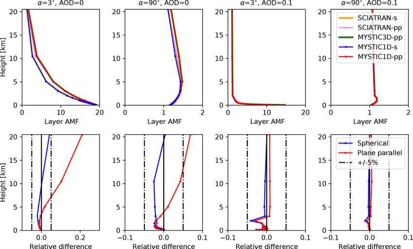
4280                       M. Schwaerzel et al.: Three-dimensional radiative transfer effects on trace gas remote sensing

Figure 1. Illustration of the difference between (a, b) 1D-layer and (c, d) 3D-box AMFs for two scenarios with (a, c) downward-looking
spaceborne and (b, d) upward-looking ground-based observations. Selected photon paths are shown as dashed lines. The 1D-layer AMFs
implicitly assume horizontally uniform atmospheric and surface properties, whereas 3D-box AMFs fully account for both vertical and
horizontal variability.

   For the comparison, we computed 1D-layer and 3D-box               above (see Table 1 in Wagner et al., 2007). Profiles of temper-
AMFs with MYSTIC in plane-parallel geometry as well as               ature, pressure, density and ozone concentration were taken
1D-layer AMFs in spherical geometry for all scenarios pre-           from the US Standard Atmosphere (United States Commit-
sented in Wagner et al. (2007). The 3D-box AMFs have not             tee on Extension to the Standard Atmosphere, 1976). Ozone
yet been implemented with spherical geometry.                        cross sections (in cm2 ) were 9.59 × 10⁻²⁰ , 6.19 × 10⁻²³ ,
   1D-layer and 3D-box AMFs were computed for five wave-             1.36 × 10⁻²² , 5.60 × 10⁻²² and 4.87 × 10⁻²¹ at 310, 360,
lengths (310, 360, 440, 477, 577 nm), seven elevation angles         440, 477 and 577 nm, respectively. Other atmospheric ab-
(1, 2, 3, 6, 10, 20, 90◦ ) and three aerosol scenarios (aerosol      sorbers were ignored. Further details can be found in Wag-
extinction of 0.0, 0.1 and 0.5 km−1 ). For the aerosol sce-          ner et al. (2007). For each scenario, we traced 1 million
narios, an aerosol layer was prescribed between 0 and 2 km           photons, which balances statistical noise expected from a
with an asymmetry parameter of 0.68 and a single-scattering          Monte Carlo approach with computation time. The computed
albedo of 1.0. No aerosols were prescribed above 2 km. For           3D-box AMFs were integrated horizontally to obtain 1D-
the simulations, 17 vertical layers were used with a thickness       layer AMFs that can be compared with the 1D-layer AMFs
of 100 m below 1000 m and a thickness of mostly 1000 m               from other models. MYSTIC was mainly compared to SCIA-

Atmos. Meas. Tech., 13, 4277–4293, 2020                                                https://doi.org/10.5194/amt-13-4277-2020
M. Schwaerzel et al.: Three-dimensional radiative transfer effects on trace gas remote sensing 4281
TRAN (Version 2.2; Rozanov et al., 2005). SCIATRAN was scenarios. This local maximum is caused by multiple scatter-
chosen because it agrees well with the mean of the models ing, which contributes to the horizontal light paths in those
in Wagner et al. (2007), and because it is based on the dis- layers. The reduction towards the surface in the latter scenar-
crete ordinate method to solve the radiative transfer equation, ios is due to the low surface albedo. For an elevation angle
which is fundamentally different from a Monte Carlo solver, of 3◦ , AMFs are high close to the ground because of the long
and finally because it offers both plane-parallel and spherical light path in the layers due to the low elevation angle. Since
solutions. In addition, we compared MYSTIC to the mean aerosols increase scattering, photon path lengths and corre-
of eight of nine RTMs in the comparison study. The PROM- spondingly 1D-layer AMFs are low in the lowest 2 km, when
SAR/Italy model was not included because of its large devi- an aerosol layer is present.
ation from the mean (see Wagner et al., 2007, for details). 1D-layer AMFs computed with spherical and plane-
parallel geometry show noticeable differences for long wave-
3.2 Validation results lengths and low aerosol extinction, especially at altitudes
above 5 km where extinction coefficients are small (see
The comparison of 1D-layer AMF profiles calculated with upper- and lower-left part in Fig. 3). In plane-parallel ge-
the MYSTIC 1D modules with SCIATRAN for the 67 obser- ometry, if one of these photons is traveling horizontally, it
vation scenarios used in Wagner et al. (2007) is summarized will strongly contribute to increase the mean photon path in
in Fig. 2 in the form of a scatter plot. The horizontally in- that specific layer. In spherical mode, the same photon would
tegrated AMFs from MYSTIC’s 3D module perfectly agree change layer because of the curved atmospheric layers, and
with its 1D module with plane-parallel geometry within the therefore its contribution to the mean photon path will be di-
statistical noise of the Monte Carlo approach. When tracing vided between the crossed layers. Furthermore, in a curved
1 million photons, the difference between 1D and 3D mod- atmosphere, the zenith angle of the photon, which was ini-
ule was smaller than 0.5 %. Therefore, only results from the tially traveling horizontally, will increase. At low altitude,
1D module were plotted against the SCIATRAN results. The these effects are smaller, and, conversely, 1D-layer AMFs
agreement between MYSTIC and SCIATRAN is very good computed with spherical and plane-parallel geometry agree
for almost all scenarios with relative differences mostly be- better (mostly < 5 %).
low 5 %. Overall, 97 % of the compared points are within a AMF profiles calculated with MYSTIC generally agree
relative difference of 5 % for spherical geometry and 92 % very well with those calculated with SCIATRAN with rel-
for plane-parallel geometry. The mean of the relative differ- ative differences mostly smaller than 5 %. However, signifi-
ences for spherical geometry is 0.9 % and its standard devi- cant differences (up to 23 % relative difference) are seen be-
ation 2.0 %, and for the plane-parallel geometry the mean is tween the plane-parallel solutions of the two models above
0.3 % with a standard deviation of 2.7 %. 5 km for the scenarios without aerosols at 577 nm (Fig. 3). In
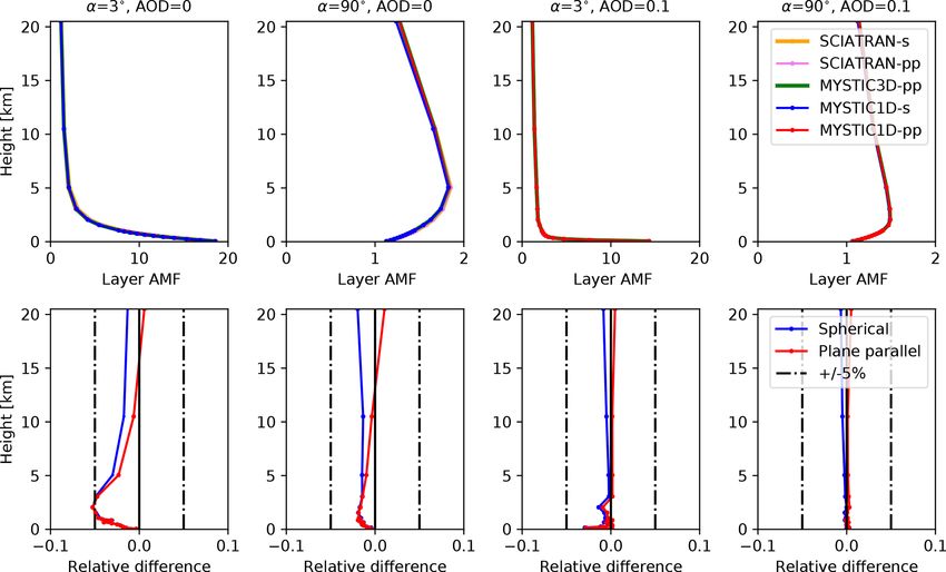
To illustrate the differences in AMF profiles between the contrast to the plane-parallel case, the spherical solution of
two RTMs, we selected four scenarios with a wavelength MYSTIC is in good agreement with the spherical solution of
of 577 nm, because at this wavelength we observe compara- SCIATRAN. The difference between SCIATRAN plane par-
tively large differences between the two models. To illustrate allel and MYSTIC plane parallel is attributed to the different
a usual scenario with low difference, we also selected the solution methods of the radiative transfer equation. A pos-
same scenarios but with a 360 nm wavelength. The upper row sible explanation is the following: in discrete ordinate meth-
of Fig. 3 (scenario at 577 nm) and Fig. 4 (scenario at 360 nm) ods, the directions of the radiation field are discretized and do
shows MYSTIC 1D-layer AMF profiles for the selected sce- not include the exact horizontal direction, for which in plane-
narios with a low elevation angle of 3◦ and a high eleva- parallel geometry the photon path length becomes extremely
tion angle of 90◦ (zenith) without and with aerosols, respec- large in an optically thin medium like the higher atmosphere.
tively. For comparison, the corresponding profiles computed In a Monte Carlo model, this horizontal direction is included;
with SCIATRAN are also shown. The lower row presents therefore the 1D-layer AMF might be larger. This hypothe-
the relative differences between MYSTIC and SCIATRAN. sis could be tested by including more streams (discrete direc-
Since plane-parallel and spherical modes have different geo- tions) in SCIATRAN and verifying if the solution approaches
metrical assumptions, we compare plane-parallel models and the higher AMFs from the MYSTIC solution.
spherical models separately. The simulations for the same scenarios but with 360 nm
In the upper atmosphere, the 1D-layer AMFs decrease wavelength agree very well with SCIATRAN for both spheri-
with altitude in all scenarios (Figs. 3 and 4), because the at- cal and plane-parallel geometries (relative difference < 5 %).
mospheric density is decreasing, which lowers the amount The differences mentioned above are much smaller at this
of scattering and, correspondingly, the mean photon path wavelength because atmospheric scattering events increase
length. In the lowest layers, however, the profile shapes are with lower wavelength and thus, prevent those very long pho-
different for the two elevation angles with a rapid decrease ton paths. We also investigated a scenario with a wavelength
with altitude in the low elevation angle scenarios and a local of 440 nm, which is a typical wavelength of the window used
maximum between 2 and 5 km in the high elevation angle for NO2 fitting (see Fig. S4 in the Supplement), for which
https://doi.org/10.5194/amt-13-4277-2020 Atmos. Meas. Tech., 13, 4277–4293, 2020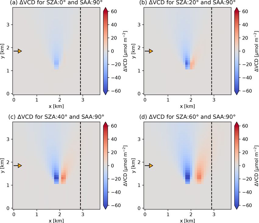
4282                        M. Schwaerzel et al.: Three-dimensional radiative transfer effects on trace gas remote sensing

Figure 2. Scatter plots of MYSTIC 1D-layer AMFs computed with (a) spherical and (b) plane-parallel geometries against 1D-layer AMFs
computed with SCIATRAN (a) spherical and (b) plane parallel for 67 MAX-DOAS scenarios with 17 layers (1139 points). The solid black
lines are the respective regression fits to the points.

Figure 3. Upper row: MAX-DOAS AMF profiles for MYSTIC 1D spherical geometry (s), 1D plane-parallel geometry (pp) and 3D plane-
parallel geometry (pp) for two selected elevation angles of 3 and 90◦ , a SZA of 20◦ , with and without aerosol for radiation at 577 nm.
Corresponding profiles computed with the SCIATRAN RTM are shown for comparison. Lower row: profile of relative differences of MYS-
TIC and SCIATRAN results in spherical (s) and plane-parallel geometry (pp) (Wagner et al., 2007).

MYSTIC and SCIATRAN also agree very well (< 5 % rela-                    Overall, MYSTIC agrees very well with SCIATRAN with
tive difference), but as for simulations at 577 nm discussed          differences mainly smaller than 5 %. An exception is the high
above, the simulations at 440 nm show significant differ-             elevation scenario without aerosols, where the plane-parallel
ences between plane-parallel and spherical geometry for lay-          solutions of MYSTIC and SCIATRAN differ by up to 23 %
ers above 5 km. These differences are, however, smaller than          for a wavelength of 577 nm at altitudes above 5 km. It should
at 577 nm because the optical thickness of Rayleigh scatter-          be noted that for these cases the 1D-layer AMFs are very
ing is higher at 440 nm.                                              small, and therefore the absolute differences, which are rel-

Atmos. Meas. Tech., 13, 4277–4293, 2020                                                 https://doi.org/10.5194/amt-13-4277-2020
M. Schwaerzel et al.: Three-dimensional radiative transfer effects on trace gas remote sensing                                    4283

Figure 4. Upper row: MAX-DOAS AMF profiles for MYSTIC 1D spherical geometry (s), 1D plane-parallel geometry (pp) and 3D plane-
parallel geometry (pp) for two selected elevation angles of 3 and 90◦ , a SZA of 20◦ , with and without aerosol for radiation at 360 nm.
Corresponding profiles computed with the SCIATRAN RTM are shown for comparison. Lower row: profile of relative differences of MYS-
TIC and SCIATRAN results in spherical (s) and plane-parallel geometry (pp) (Wagner et al., 2007).

evant for most applications, are also small. The 1D-layer             tation of the spatial distribution of the sensitivity of the mea-
AMFs computed with MYSTIC also agree very well with                   surements.
the other models presented in Wagner et al. (2007). Differ-              To illustrate the 3D distribution of 3D-box AMFs for a typ-
ences larger than 5 % are mainly attributable to differences          ical MAX-DOAS measurement, we simulated 3D-box AMFs
between plane-parallel and spherical solutions (see the Sup-          at 450 nm for two scenarios with low and high aerosol opti-
plement). When comparing MYSTIC with the mean of the                  cal depth, which correspond to a visibility of 50 and 10 km in
models, 88.3 % of the compared points are within a relative           the planetary boundary layer (PBL), respectively. A value of
difference of 5 % for spherical geometry, 81.5 % for plane-           450 nm is a typical wavelength for light absorption by NO2 .
parallel geometry, and 97.5 % for the mean of plane-parallel          The instrument points northwards with an azimuth angle of
and spherical geometry. The mean of spherical and plane-              180◦ and an elevation angle of 5◦ . The solar azimuth angle
parallel geometry agrees best because the models in Wag-              (SAA) is 344.7◦ (164.7◦ relative azimuth angle), and the so-
ner et al. (2007) represents a mixture of spherical and plane-        lar zenith angle (SZA) is 24.6◦ . The MYSTIC input file is
parallel solutions.                                                   provided in the Supplement.
                                                                         Figure 5a and b show the 3D-box AMFs in the plane of the
                                                                      line of sight of the instrument for the two scenarios. In both
                                                                      cases, 3D-box AMFs are highest along the line of sight and
4   3D-box AMFs for MAX-DOAS observations                             reduce with distance from the instrument. Most of the pho-
                                                                      tons collected by the instrument experienced a single scatter-
MAX-DOAS is a ground-based passive remote sensing tech-               ing into the line of sight of the instrument. With increased
nique allowing the retrieval of vertical concentration profiles       aerosol amount (visibility of 10 km), photons scattered into
of trace gases and aerosols (Wagner et al., 2004; Frieß et al.,       the line of sight far away from the instrument have a high
2006; Irie et al., 2011; Hönninger and Platt, 2002). Informa-         chance of being scattered out again. As a result, the sensi-
tion about the vertical distribution is obtained by measuring         tivity rapidly (within a few kilometers) decreases along the
spectra at a prescribed sequence of elevation angles. Obser-          line of sight with increasing distance from the instrument.
vations at different elevation angles have different sensitivity      Multiple scattering becomes more important in this scenario,
to the concentration in a given vertical layer. The 3D-box            which explains the enhanced sensitivity to layers below and
AMFs as computed by MYSTIC are particularly suitable to               above the line of sight within a distance of up to 4 km of the
illustrate this, because 3D-box AMFs are a direct represen-           instrument. The decrease in AMF with distance is further il-

https://doi.org/10.5194/amt-13-4277-2020                                                 Atmos. Meas. Tech., 13, 4277–4293, 2020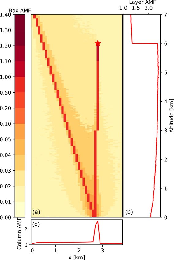
4284 M. Schwaerzel et al.: Three-dimensional radiative transfer effects on trace gas remote sensing
Figure 5. Cross section of 3D-box AMFs for a MAX-DOAS scenario with an instrument (black triangle) at the ground (z = 0 km, x = 20 km,
y = 3 km) pointing northwards and slightly upwards at a viewing angle of 5◦ . The sun is at an azimuth angle of 344.7◦ and a zenith angle
of 24.6◦ . The relative azimuth angle between sun and viewing direction is 164.7◦ . AMFs were simulated with two aerosol scenarios: a
rural-type aerosol representative of spring–summer conditions in the aerosol layer (0–2 km), with a visibility of (a) 50 km and a visibility of
(b) 10 km and a background aerosol above 2 km. Decay of vertically integrated AMFs with distance to the instrument is visualized (c) for the
same scenarios with standard (red) and high aerosols (blue) as in panels (a) and (b). The altitude of the line of sight as a function of distance
is shown in black.
lustrated for the two scenarios in Fig. 5c, which shows the signal originated from photons crossing neighboring boxes.
vertically integrated AMFs (in the aerosol layer) as a func- For the high-aerosol scenario with enhanced scattering, the
tion of distance y to the instrument normalized with AMFs part of the signal originating from the main line was corre-
integrated horizontally in y direction. The figure also shows spondingly lower, between 30 % and 41 %. The lower values
the height of the main optical path as a function of y. correspond to the scenarios with higher relative azimuth an-
To illustrate the horizontal spread of the sensitivity of the gles.
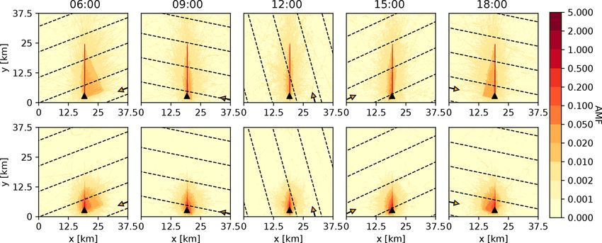
MAX-DOAS measurements in the PBL, Fig. 6 shows hor- Depending on the viewing direction of the instrument rel-
izontal distributions of vertically integrated 3D-box AMFs ative to the position of nearby emission sources, this tem-
(0–2 km) for the same scenarios with low (top row) and high porally varying spatial sensitivity could introduce a diurnal
(bottom row) aerosols and for five different sun positions cor- cycle in the measurement even when the trace gas concentra-
responding to different times of the day on 21 July in the city tion field was constant in time. Understanding the horizontal
of Zurich. The horizontal distribution of AMFs shows high distribution of the sensitivity to NO2 and its variation in time
values not only along the line of sight of the instrument but is thus particularly important for the interpretation of MAX-
also in a surrounding region, which is up to a few kilometers DOAS observations in polluted regions like cities with strong
wide. This region is wider for larger relative azimuth angles NO2 gradients, for which 3D-box AMFs can be a valuable
and is inclined towards the direction of the sun. The simu- tool.
lations show not only that the MAX-DOAS measurements
are sensitive to NO2 along the line of sight but also that they
are also influenced by neighboring regions a few kilometers 5 3D-box AMFs for airborne observations
away.
For the different scenarios, we evaluated which part of In this section, we demonstrate the effect of the spatial vari-
the signal originated from a 0.25 km wide region centered ability in 3D-box AMFs on airborne NO2 imaging spec-
on the northward pointing line of sight (referred to as main troscopy. For this purpose, we simulated a NO2 plume emit-
line in the following) and which part crossed boxes outside ted from a stack to generate a scenario with a distinct three-
this range. For the low-aerosol scenario, between 63 % and dimensional trace gas structure. An airborne spectrometer
70 % originated from the main line. Thus, up to 37 % of the was then assumed to fly parallel to the plume axis and to
sample the plume in the across-track direction (see dashed
Atmos. Meas. Tech., 13, 4277–4293, 2020 https://doi.org/10.5194/amt-13-4277-2020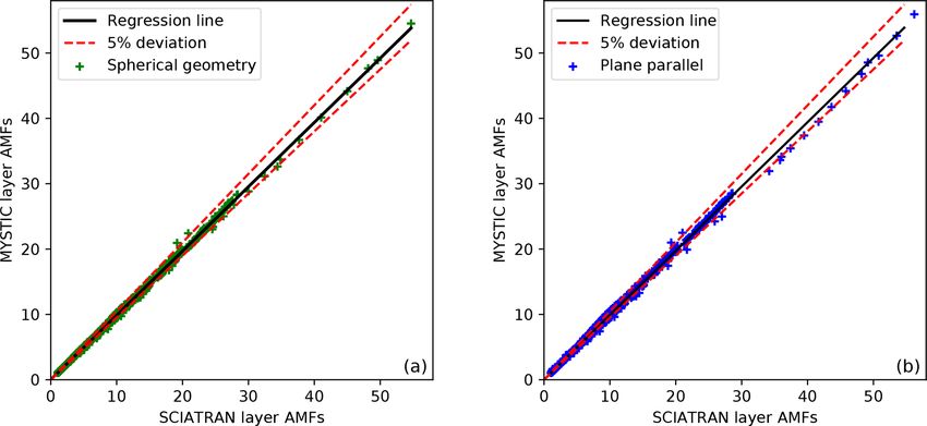
M. Schwaerzel et al.: Three-dimensional radiative transfer effects on trace gas remote sensing                                          4285

Figure 6. Top: vertically integrated 3D-box AMFs in the PBL (z < 2.0 km) for an instrument at the ground pointing northwards with an
instrument zenith angle of 5◦ for different times of the day on the 21st of June in Zurich. Solar zenith angles are 77.4, 47.5, 24.6, 38.6 and
68.5◦ , and solar azimuth angles are 249.0, 281.5, 344.7, 65.2 and 101.7◦ . The arrows point away from the sun, and the dashed lines show
the direction of photons coming from the sun. AMFs were simulated with a rural-type aerosol representative of spring–summer conditions
in the aerosol layer (0–2 km) with a visibility of 50 km and a background aerosol above 2 km. Bottom: same as above but for a scenario with
increased aerosol (visibility of 10 km).

lines in Fig. 8). We illustrate the distinct 3D-structure of the            Using MYSTIC, we computed the SCDs that would be
sensitivity of the measurements to NO2 (as represented by                observed from an airborne push-broom spectrometer flying
the 3D-box AMFs) and demonstrate the limitations of using                parallel to the plume axis from south to north at an altitude
1D-layer AMFs for such observations.                                     of 6 km. The field of view in the across-track direction of
                                                                         the instrument covers the full x-direction of the model do-
5.1   Synthetic observations of a NO2 stack emission                     main. The SCDs were obtained by computing 3D-box AMFs
      plume                                                              for each single observation (i.e., for each ground pixel) and
                                                                         multiplying these AMFs with the 3D NO2 field from the sim-
The NO2 plume was computed with the Graz Lagrangian                      ulation (which corresponds to the numerator in Eq. 5).
dispersion Model (GRAL) (Oettl, 2015) for a 262.5 m tall                    As an example, Fig. 7 illustrates the 3D-box AMFs for
stack located at x = 1.9 km and y = 1.3 km. NO2 molecules                an instrument pointing downwards at a zenith angle of 4.8◦
were released at this altitude at a constant rate of 40 kg h−1 .         and an azimuth angle of 90◦ . The sun is placed in the west
NOx chemistry was ignored for simplicity. The model do-                  (SAA = 90◦ ) at a SZA of 20◦ – i.e., the instrument is fac-
main had a size of 4 km × 4 km and extended from the sur-                ing the sun. The figure shows the 2D cross section of 3D-box
face to 21 km altitude. The simulated NO2 was sampled on an              AMFs in the principal plane of the observations, which aligns
output grid with a 100 m horizontal resolution and 20 vertical           with the x–z plane in this geometry. Figure 7b and c show
levels with 25 m resolution from 0 to 500 m. For the simula-             the horizontally and vertically integrated 3D-box AMFs, i.e.,
tion we assumed neutral atmospheric stability and southerly              layer and column AMFs, respectively. The layer AMFs are
wind with a speed of 5 m s−1 at 12 m above ground. The full              identical to 1D-layer AMFs. The 3D-box AMFs are high
vertical wind profile is generated within the model based on             along the line of sight of the instrument and largest just below
similarity theory. The NO2 background from the US Stan-                  the aircraft. Most photons travel directly along the geometric
dard Atmosphere (United States Committee on Extension to                 path from the sun to the ground pixel and then to the instru-
the Standard Atmosphere, 1976) was added to the simulated                ment. Although 3D-box AMFs are highest along the geomet-
NO2 field, which was extended to 21 km altitude (see verti-              ric path due to the relatively bright surface, a non-negligible
cal resolution profile in the Supplement). The resulting NO2             fraction of photons is scattered into the line of sight without
VCDs are shown in Fig. 8a. In the following, the simulated               reaching the surface, leading to an increase in 3D-box AMFs
NO2 concentration field and the corresponding NO2 VCDs                   within a parallelogram bounded by the line of sight and the
are referred to as the true NO2 field and as the true total              position of the sun.
VCD, respectively. The true VCD will be used as a refer-                    The column AMFs (Fig. 7c) are highest close to the in-
ence to demonstrate the limitations of 1D radiative transfer             strument and decrease with distance to the instrument in the
calculations.                                                            −x direction due to atmospheric scattering. After the “re-
                                                                         flection point”, values continue to decrease with distance to

https://doi.org/10.5194/amt-13-4277-2020                                                     Atmos. Meas. Tech., 13, 4277–4293, 2020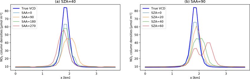
4286                          M. Schwaerzel et al.: Three-dimensional radiative transfer effects on trace gas remote sensing

                                                                          Table 1. MYSTIC input parameters for the emission stack scenario.

                                                                                  Parameter                                    Value
                                                                                  Wavelength (nm)                                 460
                                                                                  Solar zenith angle (◦ )              0, 40, 20, 60
                                                                                  Solar azimuth angle (◦ )           90, 0, 180, 270
                                                                                  Viewing zenith angle (◦ )                 0 to 26.6
                                                                                  Viewing azimuth angle (◦ )                  90/270
                                                                                  Surface albedo                                   0.2
                                                                                  Aircraft position x (km)                         2.9
                                                                                  Aircraft position y (km)                        0–4
                                                                                  Aircraft position z (km)                           6
                                                                                  Domain size (boxes)                  40 × 40 × 47
                                                                                  Horizontal resolution (m)                     100.0
                                                                                  Vertical resolution (0–7 km) (m)                  25

                                                                          putational cost of calculating 3D-box AMFs is considerably
                                                                          larger than for 1D-layer AMFs. The computational time for
                                                                          calculating 3D-box AMFs for the scenarios here (see Table 1
                                                                          with SZA = 20◦ , SAA = 90◦ , VAA = 90◦ and VZA =2◦ ) is
                                                                          around 218 s with 1 million photons using a single core of our
                                                                          local machine (Intel Xeon W-2175 CPU @ 2.5 GHz). The
                                                                          computational time for the corresponding 1D-layer AMFs is
                                                                          only about 4 s with 1 million photons. Note, however, that
                                                                          even less photons would be sufficient to obtain a similar noise
                                                                          level as for the 3D-box AMFs.
                                                                             The SCDs computed for the scenario with the sun illumi-
Figure 7. The 3D-box AMFs cross section at y = 1.4 km for the             nating the scene from the west at a solar zenith angle of 40◦
aircraft scenario presented in this section. Aircraft (red star) placed   are presented in Fig. 8b. The SCDs are larger than the VCDs
at z = 6 km, x = 2.9 km and y = 1.4 km pointing eastwards. The            (panel a) because the AMFs (panel c) are generally larger
sun is at SAA = 90◦ (west) with a SZA of 20◦ . (b) Vertical profile
                                                                          than 1. The SCD plume is wider and shifted towards the east
of horizontally integrated AMFs (1D-layer AMFs). (c) Horizontal
                                                                          compared to the VCD plume. The widening is due to both
profile of vertically integrated AMFs (column AMFs). The default
properties are a rural-type aerosol in the PBL, background aerosol        geometric effects and atmospheric scattering. Geometric ef-
above 2 km, spring–summer conditions and a visibility of 50 km.           fects are caused by the fact that photons following the main
                                                                          geometric path from the sun to the surface and to the instru-
                                                                          ment may traverse the plume either on the way from the sun
the instrument but at a lower rate. Due to periodic bound-                to the surface or from the surface to the instrument (or both).
aries this decrease continues on the right of the instrument              These two pathways are separated horizontally. For high so-
(x ≥ 3.9 km). Layer AMFs (i.e., 1D-layer AMFs) (Fig. 7b)                  lar zenith angles (here SZA = 40◦ ) this leads to two SCD
are highest directly below the instrument. They change by a               maxima close to the source as seen in Fig. 8b. The westerly
factor of 2 at the altitude of the aircraft because layers be-            maximum corresponds to the direct observation of the plume
low are crossed (at least) twice by the photons, while layers             (photons reflected by the surface pass the plume on the direct
above are only crossed once.                                              way to the aircraft), whereas the easterly maximum corre-
   3D-box AMFs and corresponding SCDs were computed                       sponds to its mirror image (photons first travel through the
for four different solar zenith angles and four different rel-            plume before they get reflected at the surface and reflected to
ative azimuth angles between the sun and the plume axis                   the aircraft). This is further illustrated in Fig. 9, where two
(and flight direction). We used a default aerosol scenario with           of the three illustrated direct paths (i.e., three viewing zenith
a rural-type aerosol representative of spring–summer condi-               angles) cross the NO2 maximum – main photon path (1) and
tions in the PBL (0–2 km) and a background aerosol above                  (3) in Fig. 9. The main photon path for the observation an-
2 km (visibility of 50 km in the PBL). The parameters used                gle (2) in Fig. 9 misses the plume maximum, which is why
for the AMF calculation are summarized in Table 1. Note                   total SCD is lower for this observation. Atmospheric scatter-
that with perfect knowledge of the relative NO2 distribu-                 ing leads to an additional horizontal smoothing of the plume,
tion, the true total VCD could be reproduced exactly from                 but in the case of a medium-high surface albedo of 0.2, the
the SCDs using 3D radiative transfer calculations. The com-               geometric effects dominate.

Atmos. Meas. Tech., 13, 4277–4293, 2020                                                       https://doi.org/10.5194/amt-13-4277-2020
M. Schwaerzel et al.: Three-dimensional radiative transfer effects on trace gas remote sensing 4287
Figure 8. Airborne remote sensing of an NO2 plume emitted from a 262.5 m tall stack located at x = 1.9 km and y = 1.3 km. The aircraft
flies at an altitude of 6 km from south to north at x = 2.9 km (dashed line) parallel to the plume axis and samples the plume in the across-
track direction. The sun is located in the west (small arrow in panel a) at a zenith angle of 40◦ . The panels show (a) simulated (true) NO2
VCDs, (b) synthetic SCDs computed from the simulated NO2 distribution by applying 3D-box AMFs and (c) 3D-box AMFs computed with
MYSTIC. The second row shows (d) VCDs calculated from the SCDs using 1D-layer AMFs and the “true” NO2 profile above the ground
pixel pointed by the instrument, (e) the difference between calculated and true VCDs, and (f) total AMFs from the MYSTIC 1D module. The
third row (g–i) shows the same as panels (d)–(f) but using the background NO2 profile to compute AMFs.
5.2 Limitations of VCDs calculated from 1D-layer Figure 8f and i show the total AMFs computed with the
AMFs true and background NO2 profile, respectively. In both cases,
AMFs increase with distance from the aircraft due to the
For each scenario, total AMFs were also computed from 1D- increasing viewing zenith angle. For the true NO2 profiles,
layer AMFs, which requires a NO2 profile (Eq. 4). The most AMFs are higher inside the plume. This can be explained by
obvious approach is to use the true NO2 profile above the the fact that the measurements are more sensitive to NO2 in-
ground pixel the instrument is pointing towards, which is side the plume than to the background NO2 outside because
based on the idea that the AMF is used to convert an SCD the plume is located at an altitude where the 1D-layer AMFs
to a VCD above a ground pixel (Fig. 8d, e, f). Alternatively, are higher.
a NO2 background profile from the US Standard Atmosphere Figure 8d and g show the VCDs obtained by dividing
(United States Committee on Extension to the Standard At- the true SCDs in Fig. 8b by the 1D-layer AMFs in Fig. 8f
mosphere, 1976) was used for each ground pixel, which as- and i, respectively. Since geometric distortions and horizon-
sumes that no information on the spatial variability in NO2 is tal smoothing due to scattering cannot be corrected for when
available (Fig. 8g, h, i). using a 1D radiative transfer model, all structures seen in the
https://doi.org/10.5194/amt-13-4277-2020 Atmos. Meas. Tech., 13, 4277–4293, 20204288 M. Schwaerzel et al.: Three-dimensional radiative transfer effects on trace gas remote sensing
is equivalent to the source strength under the assumption of
steady-state conditions.
We computed line densities 300 m downstream of the
source for the true VCD field and for fields computed with
1D-layer AMFs for different solar zenith and azimuth angles.
The VCD cross sections are shown in Fig. 12. The line den-
sities were multiplied with a wind speed of 9.1 m s−1 , which
is the wind speed at the stack height of 262.5 m in the GRAL
simulation.
Table 2 summarizes the computed line densities and fluxes
for the different scenarios. In all scenarios, emissions were
significantly underestimated by 9 %–37 % (relative to the
true VCD) depending on the solar azimuth and zenith angle.
Note that the emission estimation for the true VCD is slightly
higher than the emission input for the dispersion model due
Figure 9. Schematic of the across-track measurement by the aircraft to simplification of the mass-balance approach, which does
measuring a NO2 plume (dark blue corresponding to high NO2 con- not account for the vertical variability in wind speeds across
centrations) with three main photon paths for three measurement the plume. The bias in the plume emission estimation using
geometries (1, 2, 3). 1D-layer AMFs generally increases with solar zenith angle.
This bias also depends on the solar azimuth angle. The largest
bias occurs, when the SAA is 0 or 180◦ , i.e., the instrument
SCDs are essentially preserved in the VCDs, including the is flying towards and away from the sun.
double peak structure, the widening of the plume and the hor-
izontal displacement. Figure 8e and h show the differences
6 Conclusions
in these VCDs from the true VCDs. In both cases, the lo-
cation of the plume is shifted towards the aircraft relative This study demonstrates the importance of 3D radiative
to the true position. Within the maximum of the plume, this transfer effects for a range of trace gas remote sensing ap-
displacement leads to an underestimation of the true VCDs plications such as ground-based MAX-DOAS and airborne
by −60.8 µmol m−2 when using the NO2 profile (Fig. 8e) imaging spectroscopy. To study these effects, 1D-layer and
above the ground pixel and by −54.6 µmol m−2 when using 3D-box AMFs were implemented in the Monte Carlo solver
the constant NO2 profile (Fig. 8h). MYSTIC of the libRadtran RTM. The computation of AMFs
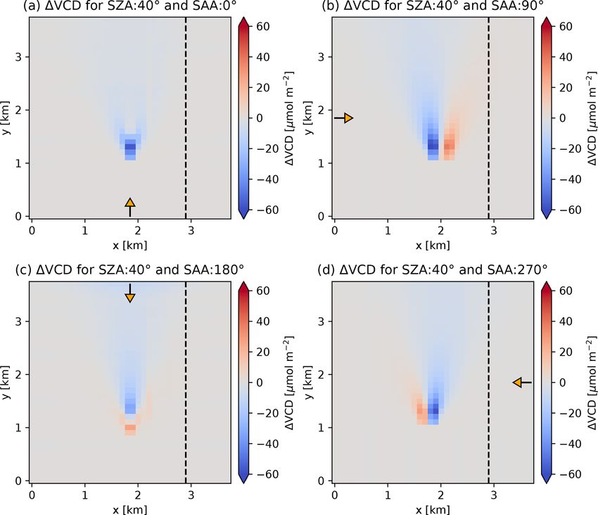
The displacement of the calculated VCD plume and the is a central component in most trace gas retrieval algorithms
magnitude of the bias depend on the position of the sun as to convert observed SCDs into VCDs, but so far these algo-
demonstrated in Figs. 10 and 11. The shift increases with rithms were limited to 1D RTMs. In the case of a horizon-
increasing SZA due to the geometric effects explained ear- tally homogeneous atmosphere and in plane-parallel geom-
lier. The relative azimuth angle between the viewing direc- etry, the 3D-box and 1D-layer AMFs perfectly agree within
tion and the sun also plays a critical role. The displacement is the statistical noise of the Monte Carlo method. They also
smaller when the aircraft is flying directly away from the sun agree very well with 1D-layer AMFs calculated with other
(SAA = 0◦ ) or towards the sun (SAA = 180◦ ) and the sun RTMs presented in a previous model intercomparison study
illuminates the scene along the plume axis, but even in these by Wagner et al. (2007).
cases it is not negligible. Biases are typically larger when the The importance of 3D effects was demonstrated for two
spatial displacement is large. examples. For a ground-based MAX-DOAS instrument, we
showed that 3D-box AMFs are highest along the line of sight
5.3 Plume flux estimation
of the instrument (representing photons that have mostly
scattered only once) but that the contribution from outside
A possible application of airborne imaging spectroscopy is
is not negligible and depends on sun position and aerosol
the estimation of NO2 emissions from point sources. Mea-
optical depth. The spatial distribution of the vertically inte-
surements from airborne spectrometers have been used, for
grated 3D-box AMFs depends on the sun position, which can
example, to estimate CO2 emissions from power plants
be important for interpreting MAX-DOAS observations, es-
(Krings et al., 2011) or CH4 emissions from coal mine venti-
pecially in urban areas or, more generally, in the vicinity of
lation shafts (Krings et al., 2013). The emissions can be esti-
pollution sources. The spatial variability in the NO2 distribu-
mated using a mass-balance approach by integrating the NO2
tion in the context of the MAX-DOAS instrument can affect
VCD enhancement above the background across the plume
the retrieval differently at different times of the day.
and multiplying this integral (referred to as line density in the
following) with a mean wind speed to obtain a flux. The flux
Atmos. Meas. Tech., 13, 4277–4293, 2020 https://doi.org/10.5194/amt-13-4277-2020M. Schwaerzel et al.: Three-dimensional radiative transfer effects on trace gas remote sensing 4289
Figure 10. Absolute difference between total VCD from synthetic SCD and 1D box AMF with solar zenith angles (SZA) of (a) 0◦ , (b) 20◦ ,
(c) 40◦ and (d) 60◦ and the true total VCD.
Table 2. Estimated NO2 emissions from the retrieved VCD fields obtained from 1D-layer AMFs under different solar zenith angle (SZA)
and solar azimuth angles (SAA).
Scenario True VCD Solar zenith angle (with SAA = 90◦ ) Solar azimuth angle (with SZA = 40◦ )
0◦ 20◦ 40◦ 60◦ 0◦ 90◦ 180◦ 270◦
Line density (g m−2 ) 1.30 1.18 1.13 1.13 1.09 0.82 1.13 1.06 1.11
Flux (kg h−1 ) 42.65 38.61 37.01 37.08 35.62 26.83 37.08 34.61 36.47
Relative bias (%) – −9.48 −13.22 −13.06 −16.49 −37.09 −13.06 −18.86 −14.49
As second example, trace gas retrievals were studied for an Our study showed that even for simple examples, 3D ef-
airborne imaging spectrometer using simulations of a NO2 fects are not negligible if the trace gas field has a high spatial
plume emitted by a stack. We showed that when using 1D- variability. This finding is particularly relevant for ground-
layer AMFs, the NO2 VCDs in the plume were significantly based and airborne remote sensing in cities, where consid-
underestimated (up to 58 %) and that the position of the ering 3D effects is likely indispensable to reduce system-
plume was artificially shifted towards the aircraft. Further- atic errors. This will be addressed in a followup study where
more, integrals of the NO2 enhancement in the across-plume the potential impact of 3D radiative transfer effects on the
direction (line densities) were also biased, which results in an horizontal smoothing of the retrieved trace gas fields will
underestimation of the NO2 emissions from the stack when also be studied. The 3D effects are also important for tomo-
using a mass-balance approach. Using 1D-layer AMFs in- graphic inversion (e.g., Frins et al., 2006; Kazahaya et al.,
duces systematic errors even if the NO2 profile above the 2008; Casaballe et al., 2020) where the application of 3D-
ground pixels is known accurately, because a 1D RTM fails box AMFs will minimize errors caused by the use of pure
to properly represent the complex light path, which is re- geometric assumptions. The high spatial resolution of the
quired if the trace gas field is not horizontally homogeneous. next generation of satellite instruments might make it nec-
essary to also consider 3D effects for space-based trace gas
https://doi.org/10.5194/amt-13-4277-2020 Atmos. Meas. Tech., 13, 4277–4293, 20204290 M. Schwaerzel et al.: Three-dimensional radiative transfer effects on trace gas remote sensing Figure 11. Absolute difference between total VCD from synthetic SCD and 1D box AMF with solar azimuth angle of (a) 0◦ , (b) 90◦ , (c) 180◦ and (d) 270◦ and the true total VCD. Figure 12. Plume VCD cross section at y = 1.6 km (0.3 km downstream of the plume) for (a) the sun at SZA = 40◦ with different SAAs and (b) for the sun in the west with different SZAs. remote sensing. Especially when considering imaging spec- 3D radiative transfer calculations require high-resolution 3D trometers with very high spatial resolution to estimate emis- distributions of trace gases and aerosols to calculate the total sions (e.g., Strandgren et al., 2020), 3D radiative transfer ef- AMF. Such fields are generally difficult to obtain. In a fol- fects should be considered and studied. However, since 3D lowup study we plan to use 3D NO2 fields from a building- radiative transfer calculations are computationally expensive, resolving urban air quality model (Berchet et al., 2017) with efficient methods need to be developed for operational appli- a detailed representation of both near-surface and elevated cations that provide an appropriate balance between accuracy (stack) emission sources to further analyze the added value and computational cost. To fully benefit from 3D-box AMFs, of 3D-box AMFs. On the other hand, measuring different az- Atmos. Meas. Tech., 13, 4277–4293, 2020 https://doi.org/10.5194/amt-13-4277-2020
M. Schwaerzel et al.: Three-dimensional radiative transfer effects on trace gas remote sensing                                          4291

imuth angles with a MAX-DOAS instrument could be used                  Boersma, K. F., Eskes, H. J., Dirksen, R. J., van der A, R. J.,
to constrain the 3D fields of trace gases (e.g., Dimitropoulou            Veefkind, J. P., Stammes, P., Huijnen, V., Kleipool, Q. L., Sneep,
et al., 2019).                                                            M., Claas, J., Leitão, J., Richter, A., Zhou, Y., and Brunner, D.:
                                                                          An improved tropospheric NO2 column retrieval algorithm for
                                                                          the Ozone Monitoring Instrument, Atmos. Meas. Tech., 4, 1905–
Code availability. The libRadtran package including the 1D ver-           1928, https://doi.org/10.5194/amt-4-1905-2011, 2011.
sion of MYSTIC is freely available on http://www.libradtran.org        Burrows, J. P., Weber, M., Buchwitz, M., Rozanov, V., Ladstätter-
(Mayer et al., 2020); the 3D MYSTIC code is available upon re-            Weißenmayer, A., Richter, A., DeBeek, R., Hoogen, R., Bram-
quest to Claudia Emde (claudia.emde@lmu.de), and the other used           stedt, K., Eichmann, K. U., Eisinger, M., and Perner, D.: The
codes are available upon request to the corresponding author.             global ozone monitoring experiment (GOME): Mission concept
                                                                          and first scientific results, J. Atmos. Sci., 56, 151–175, 1999.
                                                                       Casaballe, N., Di Martino, M., Osorio, M., Ferrari, J., Wagner, T.,
                                                                          and Frins, E.: Improved algorithm with adaptive regularization
Data availability. The data used for this study are available at
                                                                          for tomographic reconstruction of gas distributions using DOAS
https://doi.org/10.5281/zenodo.3948112 (Schwaerzel et al., 2020).
                                                                          measurements, Appl. Optics, 59, D179–D188, 2020.
                                                                       Deutschmann, T., Beirle, S., Frieß, U., Grzegorski, M., Kern, C.,
                                                                          Kritten, L., Platt, U., Prados-Román, C., Puk, ı¯te, J., Wagner, T.,
Supplement. The supplement related to this article is available on-       Werner, B., and Pfeilsticker, K.: The Monte Carlo atmospheric
line at: https://doi.org/10.5194/amt-13-4277-2020-supplement.             radiative transfer model McArtim: Introduction and validation of
                                                                          Jacobians and 3D features, J. Quant. Spectrosc. Ra., 112, 1119–
                                                                          1137, https://doi.org/10.1016/j.jqsrt.2010.12.009, 2011.
Author contributions. MS implemented the 3D-box AMF module             Dimitropoulou, E., Van Roozendael, M., Hendrick, F., Merlaud, A.,
and validated the implementation, designed and simulated the 3D           Tack, F., Fayt, C., Hermans, C., and Pinardi, G.: One year of 3-
scenarios, and wrote the paper with input from all coauthors. CE im-      D MAX-DOAS tropospheric NO2 measurements over Brussels,
plemented 1D-layer AMF module, implemented the 3D-box AMFs                in: EGU General Assembly Conference Abstracts, EGU General
together with MS, provided assistance with study design and re-           Assembly Conference, 7–12 April 2019, Vienna, Austria, 5874,
viewed the paper. TW provided the 1D-layer AMF data used for the          2019.
validation and reviewed the paper. DB, BB and AB provided critical     Emde, C. and Mayer, B.: Simulation of solar radiation during a total
feedback to the study and reviewed the paper; RM conducted and            eclipse: a challenge for radiative transfer, Atmos. Chem. Phys.,
provided the GRAL simulation; GK supervised the study, designed           7, 2259–2270, https://doi.org/10.5194/acp-7-2259-2007, 2007.
together with MS the case studies and reviewed the paper.              Emde, C., Buras-Schnell, R., Kylling, A., Mayer, B., Gasteiger, J.,
                                                                          Hamann, U., Kylling, J., Richter, B., Pause, C., Dowling, T.,
                                                                          and Bugliaro, L.: The libRadtran software package for radia-
Competing interests. The authors declare that they have no conflict       tive transfer calculations (version 2.0.1), Geosci. Model Dev., 9,
of interest.                                                              1647–1672, https://doi.org/10.5194/gmd-9-1647-2016, 2016.
                                                                       Emde, C., Buras-Schnell, R., Sterzik, M., and Bagnulo, S.:
                                                                          Influence of aerosols, clouds, and sunglint on polariza-
Financial support. This research has been supported by the Swiss          tion spectra of Earthshine, Astron. Astrophys., 605, A2,
National Science Foundation (SNSF, grant no. 172533).                     https://doi.org/10.1051/0004-6361/201629948, 2017.
                                                                       Frankenberg, C., Platt, U., and Wagner, T.: Iterative maximum
                                                                          a posteriori (IMAP)-DOAS for retrieval of strongly absorb-
                                                                          ing trace gases: Model studies for CH4 and CO2 retrieval
Review statement. This paper was edited by Folkert Boersma and
                                                                          from near infrared spectra of SCIAMACHY onboard ENVISAT,
reviewed by Frederik Tack and one anonymous referee.
                                                                          Atmos. Chem. Phys., 5, 9–22, https://doi.org/10.5194/acp-5-9-
                                                                          2005, 2005.
                                                                       Frieß, U., Monks, P., Remedios, J., Rozanov, A., Sinreich, R.,
References                                                                Wagner, T., and Platt, U.: MAX-DOAS O4 measurements: A
                                                                          new technique to derive information on atmospheric aerosols:
Berchet, A., Zink, K., Muller, C., Oettl, D., Brunner, J., Emmeneg-       2. Modeling studies, J. Geophys. Res.-Atmos., 111, D14203,
  ger, L., and Brunner, D.: A cost-effective method for simulating        https://doi.org/10.1029/2005JD006618, 2006.
  city-wide air flow and pollutant dispersion at building resolving    Frins, E., Bobrowski, N., Platt, U., and Wagner, T.: Tomographic
  scale, Atmos. Environ., 158, 181–196, 2017.                             multiaxis-differential optical absorption spectroscopy observa-
Berk, A., Anderson, G. P., Bernstein, L. S., Acharya, P. K., Dothe,       tions of Sun-illuminated targets: a technique providing well-
  H., Matthew, M. W., Adler-Golden, S. M., Chetwynd Jr., J. H.,           defined absorption paths in the boundary layer, Appl. Optics, 45,
  Richtsmeier, S. C., Pukall, B., Allred, C. L., Jeong, L. S., and        6227–6240, 2006.
  Hoke, M. L.: MODTRAN4 radiative transfer modeling for atmo-          Hendrick, F., Müller, J.-F., Clémer, K., Wang, P., De Mazière,
  spheric correction, in: Optical spectroscopic techniques and in-        M., Fayt, C., Gielen, C., Hermans, C., Ma, J. Z., Pinardi, G.,
  strumentation for atmospheric and space research III, vol. 3756,        Stavrakou, T., Vlemmix, T., and Van Roozendael, M.: Four
  348–353, International Society for Optics and Photonics, Denver,        years of ground-based MAX-DOAS observations of HONO and
  CO, USA, 1999.

https://doi.org/10.5194/amt-13-4277-2020                                                   Atmos. Meas. Tech., 13, 4277–4293, 2020
You can also read