Small Bodies: Near and Far Database for thermal infrared - Astronomy & Astrophysics
←
→
Page content transcription
If your browser does not render page correctly, please read the page content below
A&A 635, A54 (2020)
https://doi.org/10.1051/0004-6361/201936142                                                                          Astronomy
c ESO 2020                                                                                                            &
                                                                                                                     Astrophysics

            Small Bodies: Near and Far Database for thermal infrared
              observations of small bodies in the Solar System?
               Róbert Szakáts1 , Thomas Müller2 , Víctor Alí-Lagoa2 , Gábor Marton1,3 , Anikó Farkas-Takács1 ,
                                           Evelin Bányai1 , and Csaba Kiss1,3

       1
           Konkoly Observatory, Research Centre for Astronomy and Earth Sciences, Konkoly Thege Miklos ut 15-17,
           1121 Budapest, Hungary
           e-mail: szakats.robert@csfk.mta.hu
       2
           Max-Planck-Institut für extraterrestrische Physik, Giesenbachstrasse, Garching, Germany
       3
           ELTE Eötvös Loránd University, Institute of Physics, Pázmány P. s. 1/A, 1171 Budapest, Hungary

      Received 20 June 2019 / Accepted 30 December 2019

                                                                   ABSTRACT

      In this paper, we present the Small Bodies: Near and Far Infrared Database, an easy-to-use tool intended to facilitate the modelling
      of thermal emission of small bodies of the Solar System. Our database collects measurements of thermal emissions for small Solar
      System targets that are otherwise available in scattered sources and provides a complete description of the data, including all informa-
      tion necessary to perform direct scientific analyses and without the need to access additional external resources. This public database
      contains representative data of asteroid observations of large surveys (e.g. AKARI, IRAS, and WISE) as well as a collection of small
      body observations of infrared space telescopes (e.g. the Herschel Space Observatory) and provides a web interface to access this data.
      We also provide an example for the direct application of the database and show how it can be used to estimate the thermal inertia
      of specific populations, e.g. asteroids within a given size range. We show how different scalings of thermal inertia with heliocentric
      distance (i.e. temperature) may affect our interpretation of the data and discuss why the widely-used radiative conductivity exponent
      (α = –3/4) might not be adequate in general, as suggested in previous studies.
      Key words. astronomical databases: miscellaneous – minor planets, asteroids: general – infrared: general

1. Introduction                                                            (70, 100 and 160 µm, Müller et al. 2009, 2018, 2020). Recent
                                                                           reviews on the thermal emission of asteroids and more distant
The field of analysing and modelling the thermal emission of               objects by space instruments can be found in Müller et al. (2020),
asteroids has experienced substantial growth in the last decade,           Mainzer et al. (2015), and references therein.
mainly thanks to the improved availability of thermal emission
data (Delbó et al. 2015) and it will continue thanks to the rising             While the original primary goal of asteroid thermal infrared
                                                                           measurements was to derive diameters and albedos, the improve-
availability of shape models (D̆urech et al. 2015) and spatially           ment of detector sensitivity and the availability of multi-epoch
resolved in situ thermal emission data from space instruments              observations not only offer more precise diameters and albedos,
(the Hayabusa-2 and OSIRIS-REx missions, Watanabe et al.                   but also allow fort the derivation of other physical properties,
2017; Enos & Lauretta 2019).                                               such as thermal inertia and surface roughness, and, consequently,
    The typical subsolar temperatures of near-Earth asteroids are          such features as the porosity and physical nature of the regolith
∼300 K, and ∼200 K in the main belt. The thermal emission of               layer. Thermal emission measurements also provide information
these asteroids peak in the mid-infrared (10–20 µm). Although              on the YORP effect (Vokrouhlický et al. 2015) and they can con-
these wavelengths are partly available from the ground, the vast           strain the spin-axis orientation (see e.g. Müller et al. 2012, 2013,
majority of these observations are performed by space instru-              2017), as well as the temperature evolution that can alter the sur-
ments (e.g. the Akari Space Telescope and the WISE/NEOWISE                 face or subsurface composition as well as help in shape and spin
surveys Usui et al. 2011; Masiero et al. 2011). Despite their
warm surface temperatures, the modelling of near-Earth aster-              modelling (D̆urech et al. 2017), while also providing informa-
oids benefited from far-infrared observations too, such as, the            tion on diurnal temperature variations that may lead to thermal
thermal modelling of (101 955) Bennu, (308 635) 2005 YU55 ,                cracking and, thereby, produce fresh regolith (Delbó et al. 2014).
(99 942) Apophis, and (162 173) Ryugu (Müller et al. 2012,                     The interpretation of the thermal emission measurements is
2013, 2014a, 2017). Beyond Jupiter and in the transneptunian               rather complex, as the measured flux densities are strongly depen-
region, the typical surface temperatures drop from ∼100 K to               dent on the epoch of the observations through the heliocentric
30–50 K and the corresponding emission with a peak in the                  distance of the target, the distance between the target and the
far-infrared (50–100 µm) is almost exclusively observed from               observer, phase angle, aspect angle, rotational phase, and also
space. Centaurs and TNOs were suitably observable with the                 on the thermal and surface roughness properties. The actual ther-
far-infrared detectors of the Spitzer Space Telescope (mostly at           mal characteristics are not fundamental properties, as, for exam-
70 µm, Stansberry et al. 2008) and Herschel Space Observatory              ple, the thermal inertia is a function of thermal conductivity,
                                                                           heat capacity, and density, while thermal conductivity and heat
 ?
     The database is available at https://ird.konkoly.hu                   capacity both depend on the local temperature (see Keihm 1984;

                                                        Article published by EDP Sciences                                         A54, page 1 of 14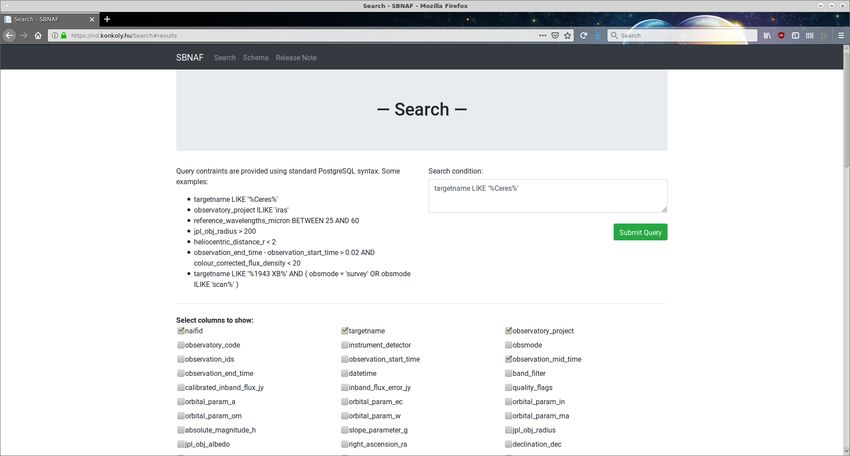
A&A 635, A54 (2020)

Keihm et al. 2012; Delbó et al. 2015; Marsset et al. 2017;             Infrared Database, and derive thermal inertias of some spe-
Rozitis et al. 2018, and references therein). Researchers work-        cific asteroid populations. Future aspects related to the database,
ing on these types of interpretations need to collect and process      including the submission of data to the IRDB, are discussed in
all of this auxiliary information to correctly interpret the thermal   Sect. 7.
emission measurements individually for all type of instruments.
     The primary goal of the Small Bodies: Near and Far
(SBNAF) Infrared Database (hereafter, IRDB) is to help sci-            2. Thermal infrared observations of asteroids and
entists working in the field of modelling the thermal emission            transneptunian objects
of small bodies by providing them with an easy-to-use tool.
Our database collects available thermal emission measurements          2.1. Database scheme
for small Solar Systems targets that are otherwise available in        The main entries in our database are the (calibrated) infrared flux
scattered sources and gives a complete description of the data,        densities and the corresponding flux density error (denoted as
including all the information necessary to perform direct scien-        f ± d f in the outline figure Fig. 1), supplemented with obser-
tific calculations and without the need to access additional exter-    vational meta data – object identifier, observatory, measure-
nal resources. The IRDB provides disk-integrated, calibrated           ment identifier, instrument-band-filter-observing mode, start and
flux densities based on careful considerations of instrument- and      end time of the observations, duration, measured in-band flux
project-specific calibration and processing steps. These multi-        (calibrated, aperture-/beam-corrected, non-linearity/saturation-
epoch, multi-wavelength, multi-aspect data allow for a more            corrected, etc.). Raw flux densities or errors and observational
complex thermophysical analysis for individual objects (e.g.           meta data are typically available in the catalogues or target-
using more sophisticated spin-shape solutions) or samples of           specific papers where we take our basic data from. These
objects. It will also allow for the combination of remote data with    papers/catalogues are listed in Sect. 2.2. All these flux densi-
close-proximity data for the same target. In addition to answer-       ties are processed (e.g. converted to [Jy] from magnitudes) and
ing direct scientific questions related to, for example, thermal       brought to a common format along with all meta data in our pro-
inertia and other surface properties of the targets, it will also      cessing (see also Fig. 1).
help in establishing celestial calibrators for instruments working         The final aim is to include data of near-Earth, main-belt, and
in the thermal infrared regime, from mid-IR to submm wave-             transneptunian objects with significant thermal measurements
lengths (see e.g. Müller et al. 2014b).                                from different satellite missions (IRAS, MSX, ISO, AKARI,
     Early versions of the database were used in several studies.      Herschel, WISE/NEOWISE) and also from the ground. In the
Marciniak et al. (2018a,b) performed a modelling of long-period        present, first public release, we include IRAS, MSX, Akari,
and low-amplitude asteroids and derived the thermal properties         Herschel, and WISE/NEOWISE observations. A more detailed
of slowly rotating asteroids; Müller et al. (2017) obtained the        description of these missions and references to available infrared
spin-axis orientation of Ryugu using data from several infrared        data are given in Sect. 2.2. The current version of the catalogue
space and ground based instruments; and the 3D shape mod-              contains 169 980 entries (see Table 1).
elling and interpretation of the VLT/Sphere imaging of (6)                 To fully utilize these measurements, we collect auxiliary data
Hebe was also supplemented by data from the infrared database          for the observations from external sources. These data are partly
(Marsset et al. 2017). Reconsiderations of the thermal emission        stored as additional useful entries (e.g. orbital elements and coor-
of Haumea (Müller et al. 2019), constrained with the occultation       dinates from JPL/Horizons) or used to calculate quantities that
results (Ortiz et al. 2017) was also performed using multi-epoch,      are necessary for the correct interpretation of the measurements
multi-mission data from the SBNAF IRDB.                                (e.g. colour correction). A list of quality comments or other rel-
     In the present version of the database, we included flux den-     evant flags are also included. The IR database is created in such
sities only at those wavelengths which are expected to be purely       a way that all available thermal measurements of our selected
thermal, with a negligible contribution from reflected solar radia-    targets are easily accessible through a simple web interface1 .
tion. This excludes, for example, the two short wavelength filters
of WISE, W1 and W2 (3.4 and 4.6 µm).
     Our final aim is to include thermal data for all Solar System     2.2. Key references and sources of data
small bodies which have been detected at thermal infrared wave-        Below we give a summary of the references and sources of aster-
lengths. The initial version of the IRDB has been created in the       oid flux densities related to each mission and telescope. A sim-
framework of the Horizon 2020 project known as Small Bodies:           ple reference code is also given for those papers or catalogues
Near and Far (COMPET-05-2015/687378, Müller et al. 2018).              that presented flux densities used for our database. These codes
     Researchers working on small body thermal emission top-           are listed in the “documents_references” field of the database for
ics are encouraged to submit their own processed and cali-             each measurement.
brated thermal infrared observations to the SBNAF IRDB. These
will be transformed to the database standards, supplemented                IRAS. A general description of the Infrared Astronomical
with auxiliary data and made available to the planetary science        Satellite (IRAS) mission can be found in Neugebauer et al.
community.                                                             (1984). A detailed summary of the IRAS mission is given in
     The structure of the paper is the following. In Sect. 2, we       the IRAS Explanatory Supplement, available at the NASA/IPAC
summarize the scheme of the SBNAF Infrared Database and give           Infrared Science Archive2 , that also covers calibration issues
a detailed summary of its resources. In Sect. 3, we describe the       (point source calibration, estimated accuracy, bright source prob-
auxiliary data that supplement the core data. A detailed list of       lems, colour correction). Asteroid fluxes are obtained from The
the database fields and SQL examples of the possible queries are       Supplemental IRAS Minor Planet Survey from Tedesco et al.
provided in Sect. 4. In Sect. 5, we investigate the impact of albe-    (2002a) [T02IRAS].
dos obtained from different resources on the colour correction
values we calculate as auxiliary data and we provide an exam-          1
                                                                           https://ird.konkoly.hu
ple application to demonstrate the capabilities of the SBNAF           2
                                                                           http://irsa.ipac.caltech.edu/IRASdocs/exp.sup/

A54, page 2 of 14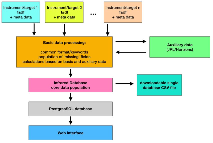
R. Szakáts et al.: Small Bodies: Near and Far Infrared Database

Fig. 1. Outline of the processing of data from the basic entries (catalogues and target-specific papers) to the web-interface of the SBNAF infrared
database.

Table 1. Observatories or missions, instruments, filters, possible observing modes, and the number of measurements with a specific instrument, in
the present version of the Infrared Database.

                  Mission      Instrument                       Filters                       Observing mode              Nobs
                  AKARI        IRC-NIR                          N4                                 IRC02                   1
                              IRC-MIR-S                    S7, S9W, S11                    Survey, IRC02, IRC11          6955
                              IRC-MIR-L                   L15, L18W, L24                   Survey, IRC02, IRC51         13 824
                  HSO            PACS                      Blue,green,red                   Chop-nod, scan map           1852
                  MSX                          MSX_A,MSX_C,MSX_D,MSX_E                             Survey                 901
                  IRAS                         IRAS12,IRAS25,IRAS60,IRAS100                        Survey               25 064
                  WISE                                         W3,W4                               Survey               121 383
Notes. Instruments on low-Earth orbits, such as AKARI, MSX and IRAS are referred to as geocentric (JPL code “500@399”), and we used the
JPL code “500@-163” for WISE and “500@-486” for Herschel.

    MSX. Mill (1994) and Mill et al. (1994) provide an overview            to as [AKARIAFC] in the IRDB. The catalogue contains data
of the spacecraft, its instruments, and scientific objectives, and         from the all-sky survey by Usui et al. (2011), slow-scan obser-
Price & Witteborn (1995), Price et al. (1998) a general descrip-           vation by Hasegawa et al. (2013), and pointed observations of
tion of the astronomy experiments. More details on the astronomy           (25 143) Itokawa and (162 173) Ryugu by Müller et al. (2014c,
experiments and the influence the spacecraft design has on these           2017). These “non-survey” modes have their special flags in the
experiments can be found in Price et al. (2001). Asteroid fluxes           “obsmode” fields (IRC02: pointed observations; IRC11/IRC51:
are obtained from The Midcourse Space Experiment Infrared                  slow scan), as defined in the AKARI Asteroid Flux Catalogue.
Minor Planet Survey catalogue from Tedesco et al. (2002b).                     Herschel. The Herschel Space Observatory mission is sum-
   AKARI. The AKARI mission is described in Murakami et al.                marized in Pilbratt et al. (2010). The Photometer Array Camera
(2007). Minor planet flux densities are obtained from the AKARI            and Spectrometer (PACS) instrument is described in Poglitsch
Asteroid Flux Catalog Ver.13 (Release October 2016), referred              et al. (2010). The photometric calibration of PACS is dis-
                                                                           cussed in Nielbock et al. (2013) (chop-nod photometric observ-
3
  https://www.ir.isas.jaxa.jp/AKARI/Archive/                               ing mode) and in Balog et al. (2014) (scan-map photometric
Catalogues/Asteroid_Flux_V1/                                               mode).
                                                                                                                                 A54, page 3 of 14
A&A 635, A54 (2020)
Flux densities of Solar System small bodies are obtained orbit at the reference epoch4 ; longitude of ascending node, Ω (◦ );
from selected publications of near-Earth asteroids and Cen- argument of perifocus, $ (◦ ); mean anomaly, M (◦ ).
taurs/transneptunian objects. – Parameters related to size and albedo: absolute magni-
tude, H (mag); slope parameter G; object’s effective radius [km];
WISE. The WISE mission is described in Wright et al.
object’s V-band geometric albedo.
(2010). Data products are summarized in the Explanatory Sup-
– Apparent position: apparent right ascension (RA) and dec-
plement to the AllWISE Data Release Products (Cutri et al.
lination (Dec) at the time of the observation, ICRF/J2000 inertial
2013).
reference frame, compensated for down-leg light-time [deg/deg];
The WISE Moving Object Pipeline Subsystem (WMOPS)
rate of change of target center apparent RA and Dec (airless). We
reported all detections of Solar System small bodies to the IAU
note that dRA/dt is multiplied by the cosine of the declination
Minor Planet Center (MPC) for confirmation, whereas the com-
[both in arcsec h−1 ].
puted in-band magnitudes were collected in the IRSA/IPAC
– Target brightness: asteroid’s approximate apparent visual
archive, namely in the Level 1b catalogues. To retrieve these
magnitude and surface brightness,
magnitudes, we queried the IPAC archive using a 1 arcsec cone
search radius around the MPC-reported tracklets, which are all APmag = H +5 log10 (∆)+5 log10 (r)−2.5 log10 ((1−G)Φ1 +GΦ2 ),
labelled “C51” by the MPC. In this way, we avoid using false
detections that may have been included in the IPAC archive (3)
(Mainzer et al. 2011). where H is the absolute brightness, r the heliocentric distance
Since we are only interested in flux densities collected during of the target, ∆ is the observer distance, and G, Φ1 and Φ2 are
the fully-cryogenic phase of the mission, we queried the WISE the slope parameter and the two base functions in Bowell et al.
All-Sky Database. The in-band magnitudes (m) were converted (1989) [mag, mag arcsec−2 ].
to in-band flux densities (h f i) as: – Heliocentric distance: heliocentric range (r, light-time cor-
rected) and range-rate (“rdot”) of the target center [AU and
h f i = h f0 i10−0.4m , (1)
km s−1 ]. In addition, the one-way down-leg light-time from tar-
where h f0 i is the zero-magnitude isophotal flux density of Vega get center to observer is also retrieved [s].
for each band, as reported in Wright et al. (2010). By defini- – Sun-Observer-Target angle: target’s apparent solar elonga-
tion, h f0 i does not require a colour correction. From the tabu- tion seen from the observer location at print-time [◦ ]. “/r” flag
lated magnitude error bar ∆m, the corresponding error bar of the indicating the target’s apparent position relative to the Sun in the
in-bad flux is given by: observer’s sky (“/T” for trailing, “/L” for leading).
– Ecliptic coordinates of the target: Observer-centered Earth
∆ f = 0.40 log10 h f i∆m. (2) J2000.0 ecliptic longitude and latitude of the target center’s
To correct for a discrepancy between red and blue calibrators apparent position, adjusted for light-time, the gravitational
observed after launch, Wright et al. (2010) suggest shifting the deflection of light and stellar aberration [deg/deg].
W3 and W4 isophotal wavelengths and correcting the isophotal – X, Y, Z Cartesian coordinates of the target body and
flux densities accordingly. Thus, we took 11.10 and 22.64 µm and observer/Earth at the time of observation in the J2000.0 refer-
31.368, and 7.952 Jy, respectively (more details in Masiero et al. ence frame defined in Archinal et al. (2011) [AU].
2011). Flux densities obtained using this procedure are referred Data from JPL Horizons are obtained by four functions in
to as [WISEASD] in the respective field of our IRDB. In this the main python script. These functions are:
release of the database, we included only those WISE measure- – get_jplh: this function obtains the ephemeris data from JPL
ments where there is also AKARI data for that object. Horizons, such as RA, Dec, r, delta, etc.
– get_jplhelements: the orbital elements of the target body are
retrieved with this function.
3. Auxiliary data – getvecs1 & getvecs2: these functions obtain the X,Y,Z posi-
tion vectors from JPL with respect to the Sun and the
In our database, in addition to the basic data available in the
observer.
resources listed above (measured (in-band) flux density and its
The following parameters are also extracted from the .csv files
uncertainty, date, instrument and filter, etc.), each measurement
obtained by these functions: H, JPL radius, albedo, and slope
is supplemented with additional (auxiliary) data, either with data
parameter. In those cases when JPL recognizes the target as a
from external resources (mainly JPL/Horizons, Sect. 3.1), as
comet and not an asteroid, T -mag (Comet’s approximate appar-
well as values calculated from other fields of the database. The
ent visual total magnitude), M1 (Total absolute magnitude)
latter include the calculation of the monochromatic flux density
parameters are extracted and used. Also, a comment is written
at a pre-defined reference wavelengths (colour correction), con-
into to the database in this case.
version of calendar date to Julian date (JD, with or without cor-
The functions use astropy.table from Astropy (Astropy
rection for light-travel time), and adding absolute flux density
Collaboration 2013, 2018) and urllib35 .
errors (Sect. 3.2). The procedures to obtain these auxiliary data
are summarized below.
3.2. Calculated values
3.1. JPL Horizons data Obtaining monochromatic flux density (colour correction).
For most of the instruments or filters included in the IRDB,
Our database uses data obtained from NASA’s JPL-Horizons ser-
colour correction is calculated using the relative response pro-
vice. These data are stored in the database and available directly
files of the specific filters and assuming an estimated effective
in the IRDB and, in some cases, also used for further calcula-
tions. We query the following parameters from JPL-Horizons: 4
Obliquity of 84381.448 arcsec with respect to the ICRF equator
– Orbital elements: semi-major axis, a (AU); eccentricity, e; (IAU76).
inclination w.r.t XY-plane, i (◦ ) (XY-plane: plane of the Earth’s 5
https://pypi.org/project/urllib3/
A54, page 4 of 14R. Szakáts et al.: Small Bodies: Near and Far Infrared Database
Table 2. Resources of Herschel Space Observatory measurements.
Near-Earth asteroids
Müller et al. (2012) [M12] (101 955) Bennu
Müller et al. (2017) [M13] (308 625) 2005 YU55
Müller et al. (2017) [M14] (99 942) Apophis
Müller et al. (2017) [M17] (162 173) Ryugu
Centaurs and transneptunian objects
Duffard et al. (2014) [D14] 16 Centaurs
Fornasier et al. (2013) [F13] (2060) Chiron, (10 199) Chariklo, (38 628) Huya, (50 000) Quaoar,
(55 637) 2002 UX25, (84 522) 2002 TC302, (90 482) Orcus, (120 347)
Salacia, (136 108) Haumea
Kiss et al. (2013) [K13] 2012 DR30
Lellouch et al. (2013) [L10] (136 108) Haumea
Lellouch et al. (2013) [L13] (20 000) Varuna, (55 636) 2002 TX300, (120 348) 2004 TY364,
(15 820) 1994 TB, (28 978) Ixion (33 340) 1998 VG44, (26 308) 1998
SM165, (26 375) 1999 DE9, (119 979) 2002 WC19, (44 594) 1999
OX3, (48 639) 1995 TL8
Lellouch et al. (2016) [L16] Pluto+Charon
Lim et al. (2010) [LIM10] (136 472) Makemake, (90 482) Orcus
Mommert et al. (2012) [MM12] 18 plutinos
Müller et al. (2010) [M10] (208 996) 2003 AZ84, (126 154) 2001 YH140, (79 360) Sila-
Nunam, (82 075) 2000 YW134, (42 355) Typhon, 2006 SX368,
(145 480) 2005 TB190
Müller et al. (2020) [M19A] (136 081) Haumea
Pál et al. (2012) [P12] (90 377) Sedna, 2010 EK 139
Pál et al. (2015) [P15] 2013 AZ 60
Santos-Sanz et al. (2012) [SS12] 15 scattered disk and detached objects
Santos-Sanz et al. (2017) [SS17] (84 922) 2003 VS 2, (208 996) 2003 AZ 84
Vilenius et al. (2012) [V12] 19 classical transneptunian objects
Vilenius et al. (2014) [V14] 18 classical transneptunian objects
Vilenius et al. (2018) [V18] 1995 SM 55, 2005 RR 43, 2003 UZ 117, 2003 OP 32, 2002 TX 300,
1996 TO 66, 1999 CD 158, 1999 KR 16
temperature (T eff ) for the target, which is calculated as: is obtained as fλ = fi /K(λ), where fi is the in-band flux density
obtained directly from the measurements and K(λ) is the colour
393.6 K correction factor, which is obtained using the spectral energy
T eff = √ (1 − pV · q)1/4 , (4)
rh distribution of the source (flux density Fν (λ)) and the relative
response of the detector/filter system (Rν (λ)) as:
where rh is the heliocentric distance (AU), pV is the V-band geo- 1
R
metric albedo and q is the standard Bowell et al. (1989) phase Fν (λc ) Fν (λ)Rν (λ)dλ
integral: q = 0.290+0.684G, where G is the slope parameter and K(λ) = 1 R ref , (5)
F ref (λ )
Fν (λ)Rν (λ)dλ
using the solar constant of 1361.5 W m−2 (Kopp & Lean 2011) ν c
and the Stefan-Boltzmann constant to get T = 393.6 K at 1 AU. where λc is the central (reference) wavelength of the filter in the
We assumed an emissivity of unity. We use T eff to calculate a photometric system and Fνref (λ) is the reference spectral energy
black body SED which we utilize during the colour correction. distribution of the photometric system (typically νFν = const.).
But in case of high-albedo objects this formula does not work The monochromatic flux density uncertainties are calculated
well (see Vilenius et al. 2018 and Brucker et al. 2009). If pV as:
is unknown or uncertain, we use pV = 0.10 (see Sect. 5). We s
note that the pV in Eq. (4) is obtained from the tabulated H 1 2
δ fλ = ∆ fi + (rabs fi )2 + (rcc fλ )2 , (6)
and D values from the Horizons JPL service. Arguably, there are K(λ)2
other sources of diameters and H values that could be used to
calculate pV but the colour correction values are not extremely where ∆ fi is the in-band flux density uncertainty and rabs is the
sensitive to large variations of pV (see Sect. 5 for further dis- absolute calibration error, usually expressed as a fraction of the
cussion of this point). We include these diameters, albedos, and in-band flux (see below). The last term contains the flux den-
H −G values in the database for the sake of reproducibility of the sity uncertainty due to the colour correction uncertainty charac-
monochromatic flux densities, but for statistical analyses with terised by rcc , which is approximately proportional to the devi-
these quantities we recommend using or at least examining other ation of the actual value of the colour correction from unity. In
sources (e.g. Delbó et al. 20176 ; Oszkiewicz et al. 2011; Veres̆ the present version, it is implemented in the following way:
et al. 2015). The colour corrected or monochromatic flux density – if 0.95 ≤ K(λ) ≤ 1.05 then rcc = 0.01;
– if 0.90 ≤ K(λ) ≤ 0.95 then rcc = 0.02;
6
https://www-n.oca.eu/delbo/astphys/astphys.html – if K(λ) ≤ 0.90 or K(λ) ≥ 1.05 then rcc = 0.03.
A54, page 5 of 14A&A 635, A54 (2020)
Fig. 2. Query of 1 Ceres, with some examples on the left.
Procedure for adding the absolute calibration error. Abso- Core 2.0 Framework. This web application communicates with
lute calibration error is calculated as described above in Eq. (6). the webserver, with the users through the webpage and with the
The rabs factor is instrument- or filter-dependent and it is deter- database itself (PostgreSQL table). The web content is gener-
mined during the flux calibration of the instrument and is ated on the server, and the users can only see the static HTML
described in instrument specific calibration papers. These rabs page in their web browser at the end. The user has the option to
values are following: download the output page as a .csv file (using the “Download”
– IRAS: 10%, 10%, 15% and 15% at 12, 25, 60 and 100 µm button).
(Tedesco et al. 2002a) The example above was generated by the following query:
– Herschel/PACS: 5%, 5% and 7% at 70, 100 and 160 µm targetname LIKE “%Ceres%” and (observatory_project
(Balog et al. 2014) LIKE “IRAS” or observatory_project ILIKE “Akari”),
– WISE: 5% in all bands (Wright et al. 2010; Rozitis et al. requiring exact, case sensitive matching with “LIKE” on “tar-
2014; Hanus̆ et al. 2015) getname” (=“Ceres”) and selecting observatories “IRAS” (exact
– MSX7 : 5%, 5%, 6% and 6% at 8.28, 12.13, 14.65 and name again with “LIKE”) and “Akari” (selecting with “ILIKE”,
21.34 µm (Egan et al. 2003) i.e. case-insensitive). In this case, the output gives the default
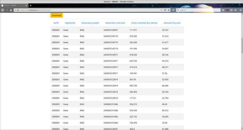
– AKARI: 5% in all bands (Usui et al. 2011; Alí-Lagoa et al. selection: “naifid”, “targetname”, “observatory_project”, “obser-
2018). vation_mid_time”, “colour_corrected_flux_density”, and “abso-
lute_flux_error”.
Numeric data types (FLOAT, DOUBLE) can be queried as
4. Database and access
follows: observation_start_time BETWEEN 2453869 AND
4.1. Main database file and web interface 2454000: selects the objects where the observation time started
between 2453869 and 2454000 (JD); observation_start_time >
From the collected data (flux densities, observational meta data, 2453869 AND observation_start_time < 2454000: returns the
and auxiliary data, see above) a PostgreSQL table is created that same results as the previous query. naifid = 2000001 : returns
is the essentially the SBNAF Infrared Database. The database all targets with “naifid” exactly equal to 2000001.
is accessible through a web interface8 (at Konkoly Observatory). For string type data: targetname ILIKE “%ceres%”:
An example is shown below, presenting the query screen (Fig. 2) selects the targets with the substring “ceres” in it, case insen-
and the resulting output screen (Fig. 3) for some selected IRAS sitive; observatory_project = “IRAS”: returns all observations
and Akari observations of 1 Ceres. where the observatory_project name matches “IRAS” exactly.
The SBNAF IRDB webpage is running on a dedicated linux The query “comments_remarks ILIKE “%comet%””
machine. The webserver is NGINX and the webpage itself is lists measurements of comets (currently the Akari observations
a ASP.NET Core Web Application, which uses the ASP.NET of the comet P/2006 HR30 (Siding Spring) in the D2.5 version
7
We took the absolute calibration uncertainties from Table 1 except for of the database).
band A, for which we used a more conservative 5% absolute calibration Additional examples are given on the starting page of the
error bar. web interface. The summary of the database fields is given in
8
Available at https://ird.konkoly.hu the appendix.
A54, page 6 of 14R. Szakáts et al.: Small Bodies: Near and Far Infrared Database
Fig. 3. Results listing infrared observation of 1 Ceres and displaying the default output selection: “naifid”, “targetname”, “observatory_project”,
“observation_mid_time”, “colour_corrected_flux_density”, and “absolute_flux_error”.
4.2. Alternative access approximation for objects with albedos pV . 0.30. We investi-
gated how different the colour correction factors obtained using
For those who want a more scriptable form of access to the the Horizons albedo values are from those obtained using albe-
IRDB, we will upload the database into the VizieR catalog ser- dos calculated for specific objects based on radiometry in previ-
vice (Ochsenbein et al. 2000). This database is widely used by ous studies (e.g. Mommert et al. 2012; Santos-Sanz et al. 2012;
the community and it provides an interface to search trough the Vilenius et al. 2012, 2014). This comparison was performed for
different databases, and it can be queried trough several tools, Centaurs and transneptunian objects, as in these cases significant
like Astropy’s astroquery.vizier interface or Topcat. In case of a deviations are expected from the general, low albedo values.
major update we will upload a new data release to VizieR. Figure 4 presents the colour correction factors obtained using
Also, we began the integration of the IRDB to the VESPA the albedo values from NASA/Horizons (top row), as well as
VO service9 (Erard et al. 2018). In this way our database can be those obtained from specific publications (bottom row). In gen-
accessed via EPN-TAP protocol, which is well known in the Vir- eral, the differences in the colour correction factors are negli-
tual Observatory community. VESPA also provides a great tool gible (mainly because the corrections factors typically close to
for searching trough the different data services and with its help, 1 in the surface temperature range for the Herschel/PACS fil-
the IRDB can become more accessible to researchers working ters). However, for some individual targets (e.g. those with large
on topics related to small body thermal emission. Because the heliocentric distance and relatively high albedo) the colour cor-
VEASPA service will use the same database as our webpage, rection factors may differ by 5–10%. Therefore, in the updated
the data entered there will be always up to date. version of the infrared database, we used the object-specific val-
The whole database can be downloaded directly from our ues whenever they are available.
webpage in csv format. The datafile contains a header and
exactly the same data that can be accessed via the SQL query
form. The size of the raw csv file is ∼125 MB in the current 6. Thermal inertias of asteroid populations
release.
In this section, we provide an example of how the database can
be used to study scientific questions. Namely, we show how to
5. Albedos and colour corrections of explore the dependence of thermal inertia (Γ) with temperature
(T ) or, equivalently, heliocentric distance (r), and how to com-
transneptunian objects pare populations of asteroids with different sizes. These quanti-
As described in Sect 3.1, albedo information is taken by default ties are relevant, for example, for studies of dynamical evolution
from the NASA/Horizons service. In case these albedo values where the Yarkovsky effect plays a role since it is influenced
are not known, we assumed an intermediate value of pV = 0.10 among other factors by Γ (see e.g. Bottke√et al. 2006).
to calculate the colour correction, which is a reasonable Thermal inertia is defined as Γ = ρCκ, where ρ is the
density, C the specific heat capacity, and κ the thermal con-
9
https://voparis-wiki.obspm.fr/display/VES/EPN-TAP+ ductivity of the material. Its SI unit is J m−2 s−1/2 K−1 . Most
Services thermo-physical models of asteroids used so far to constrain Γ
A54, page 7 of 14A&A 635, A54 (2020)
Fig. 4. Comparison of the colour correction factors obtained using the “default” albedo data from NASA/Horizons (upper row), and the albedos
obtained from specific publications and/or processing. B(70), G(100) and R(160) mark the 70, 100 and 160 µm filters of the PACS camera.
have assumed it is constant even though the heat conductivity is of saturation occurs in each band with horizontal lines of the cor-
itself a function of temperature. For this reason, thermal inertias responding colour.
determined from observations taken at different heliocentric dis- Next, we used the thermo-physical model of Delbó et al.
tances cannot be compared directly and must be normalised to (2007) under the Lagerros approximation (Lagerros 1996, 1998)
an agreed heliocentric distance (see, e.g. Delbó et al. 2015 for a to calculate the W3 and W4 fluxes at various heliocentric dis-
review). Assuming that heat is transported through the regolith tances (r = 1.25, 1.5, 2.0, 2.5, . . . 6.0 au) for a rotating sphere10
mainly by radiative conduction within the spaces between the with rotation period P = 6 h,
grains (Jakosky 1986; Kuhrt & Giese 1989), we have κ ∝ T 3 and Bond albedo A = 0.03, surface roughness rms = 0.6
hence Γ ∝ r−3/4 (see also the discussion by Delbó et al. 2007). (the default value for main belt asteroids chosen by Müller
We can then write & Lagerros 1998; Müller 2002), and different thermal inertias at
1 au. We sampled Γ0 = 10, 30, 50, 100, 150, 200 J m−2 s−1/2 K−1
Γ(r) = Γ0 rα , (7) and α = 0, −0.75 and −2.20, and used Eq. (7) to compute the
where Γ0 is the value at 1 au, r is expressed in au, and α = −3/4 corresponding Γ(r) for each case.
is the classically-assumed radiative conductivity exponent. Figures 5–7 show the W3 and W4 data and the best fit-
Rozitis et al. (2018) studied three eccentric near-Earth aster- ting models corresponding to α = 0, −0.75, and −2.20. The
oids observed by WISE more than once at a wide range of r and best Γ0 in each case increases with α, namely 10, 50 and
showed that −3/4 may not be appropriate in general. Instead, 150 J m−2 s−1/2 K−1 . These models appear to reproduce the data
they found that each one of their targets required different expo- trend reasonably well considering the numerous approxima-
nents to fit their Γ-vs.-r plots, namely α = −2.2, −1.5, and −0.92, tions that we made. To establish a quantitative comparison, we
although only the error bars of the first case, (1036) Ganymed, averaged the data within 0.5 au-wide heliocentric distance bins
were incompatible with the “classical” α = −3/4. This effect centred at 2.0, 2.5, . . . 4.5 au, and used these averages ( fbin )
requires further studies. Below, we propose ways to use our and standard deviations (σbin ) to calculate the χ2 for each
model (Fbin ) as χ2 = bins (Fbin − fbin ) /σbin 2 . Considering two
P
database to examine how α affects our interpretation of the ther-
mal IR observations. degrees of freedom, α and Γ0 , all three cases produced reduced
With our database, we can readily select the thermally dom- χ2 between ∼4.5 and 5 indicating that the data are fit at 2.2 sigma
inated WISE W3 and W4 fluxes of a group of asteroids within only in average. Hence, we cannot simultaneously optimise α
a given size and albedo range and compare how models with and Γ0 with this approach given the current lack of “ground-
different pairs of values of Γ and α fit the observations. First, truth” information for objects in this size range.
we took 10-km, low-albedo asteroids. To account for uncertain- Nonetheless, it is still worth putting these models in the con-
ties, we queried the database for all W3 and W4 colour-corrected text of other populations. For example, if α = 0 was to be
fluxes of objects in the size range 9 km ≤ D ≤ 11 km with vis- confirmed, we would conclude that the typical Γ0 ’s of 10-km
ible geometric albedos pV ≤ 0.12. This sample includes ∼4000 10
More specifically, we averaged the fluxes of a prograde sphere and
fluxes per band, corresponding to about 300 asteroids, the vast a retrograde sphere with pole ecliptic latitudes of ±90◦ , respectively. In
majority of which are main-belt asteroids. Figure 5 shows these addition, to reproduce WISE’s observation geometry, the model fluxes
fluxes plotted against heliocentric distance at the epoch of obser- are computed for an observer-sun-asteroid configuration in quadrature
vations. For reference, we also show the fluxes at which the onset assuming a circular orbit on the ecliptic.
A54, page 8 of 14R. Szakáts et al.: Small Bodies: Near and Far Infrared Database
1000 D = 10 km W3 data 1000 D = 10 km W3 data
W4 data W4 data
Γ(1 au) = 10 J m-2s-1/2K-1 W3 model Γ(1 au) = 50 J m-2s-1/2K-1 W3 model
α = 0 (Γ = constant) W4 model α=-3/4 W4 model
100 100
Flux density (Jy)
Flux density (Jy)
10 W4 saturation onset 10 W4 saturation onset
1 W3 saturation onset 1 W3 saturation onset
0.1 0.1
0.01 0.01
1 2 3 4 5 6 1 2 3 4 5 6
Heliocentric distance (au) Heliocentric distance (au)
Fig. 5. WISE W3 and W4 colour-corrected fluxes of 10-km aster- Fig. 6. Same as Fig. 5 but with α = −3/4 and Γ0 = 50 J m−2 2s−1/2
1/2K−11.
oids vs. heliocentric distance (blue and ochre empty circles). The pur-
ple and green lines are the corresponding model fluxes with Γ0 =
10 J m−2 s−1/2 K−1 and α = 0. For reference, since we have excluded 1000 D = 10 km W3 data
W4 data
partially saturated fluxes from the analysis (cf. Fig. 8, left panel), we Γ(1 au) = 150 J m-2s-1/2K-1 W3 model
also indicate the fluxes at which saturation occurs in each band (Cutri α=-2.2 W4 model
100
et al. 2012).
Flux density (Jy)
10 W4 saturation onset
asteroids would be a factor of 5 lower than that of the Moon’s
(∼50 J m−2 s−1/2 K−1 ). This would be unexpected because so far 1 W3 saturation onset
such low Γs have only been found among the largest asteroids
(e.g. Müller 2002; Mueller et al. 2006; O’Rourke et al. 2012; 0.1
Delbó & Tanga 2009; Hanus̆ et al. 2018), but we cannot rule
the possibility out from this approach alone. Among the models
with α = −3/4, the best Γ0 is very close to the lunar value and 0.01
the average Γ0 of the nine 10-km objects in Table A.3 of Hanus̆
et al. (2018), namely ∼58 J m−2 s−1/2 K−1 . However, this does not 1 2 3 4 5 6
confirm α = −3/4 as the best value for 10-km either. Based on Heliocentric distance (au)
previous modelling reviewed by Delbó et al. (2015); see their Fig. 7. Same as Fig. 5 but with α = −2.2 and Γ0 = 150 J m−2 s−1/2 K−1 .
right panel of Fig. 9; we would actually expect higher Γ0 s for
the “classical” α value, specifically in the ∼300 J m−2 s−1/2 K−1
(the role of size is further discussed below). A larger sample of and a finer and more complete sampling of Γ, α, and P, it might
10-km asteroids with accurate shapes and modelled Γs would be possible to obtain a model with a high “goodness of fit” (see
be needed to establish a more conclusive result. We would also e.g. Press et al. 1986).
need many more high-quality shape models of highly eccentric We have not considered the completeness of the samples and
objects to enable additional studies like Rozitis et al. (2018) in we emphasise that the database does not currently contain the
order to constrain α, given its crucial impact on the Γ0 values and full WISE catalogue, but only the data pertaining to those objects
ultimately on their physical interpretation, especially in the light that are featured in the AKARI catalogue. The AKARI catalogue
of the results from the space missions. is complete in the Main Belt down to sizes 20 km (Usui et al.
The approach illustrated here does enable the comparison 2013, 2014), but contains fewer Hildas/Cybeles/Jupiter Trojans
of thermal inertias of differently sized populations if we keep in the L18W band. Also, in future works, we will incorporate the
all other parameters equal. For instance, we have about 2500 full WISE catalogue into the database to have more NEAs and
observations of the ∼100 objects with sizes of 75 km that are members of populations beyond the main belt.
featured both in the WISE and the AKARI catalogues (see
Sec. 2.2). With α = −2.20, we require a lower Γ0 to fit 75-
km asteroid data (50 J m−2 s−1/2 K−1 ) than 10-km asteroid data
(150 J m−2 s−1/2 K−1 ). The W3 and W4 (left panel) and S9W and 7. Future updates of the SBNAF Infrared Database
L18W (right panel) data and corresponding model fluxes for 7.1. Planned updates
75-km asteroids are shown in Fig. 8. Although there are fewer
objects in this size range and removing partially saturated data A full assessment of all Herschel/PACS main belt asteroid obser-
introduces an artefact in the W3 data trend, the conclusion that vations were performed in the framework of the Small Bodies:
smaller asteroids have higher thermal inertias is robustly sup- Near and Far Horizon 2020 project (Müller et al. 2018). Far-
ported, at least when comparing the 10–75-km diameter range. infrared flux densities obtained from these measurements will
Finally, some of the effects not accounted for by our simpli- be made public with the next release of the database. Infrared
fying assumptions could be added into the modelling in future data from serendipitous observations of bright main belt aster-
work, such as, a large set of shapes with different elongations oids with the Herschel/PACS and SPIRE photometer detectors
or degrees of irregularity and spin pole orientations. With these, are also planned to be added.
A54, page 9 of 14A&A 635, A54 (2020)
1000 D = 75 km W3 data 1000 D = 75 km S9W data
W4 data L18W data
Γ(1 au) = 50 J m-2s-1/2K-1 W3 model Γ(1 au) = 50 J m-2s-1/2K-1 S9W model
α=-2.2 W4 model α=-2.2 L18W model
100 100
W4 saturation onset
Flux density (Jy)
Flux density (Jy)
10 10
W3 saturation onset
1 1
0.1 0.1
0.01 0.01
1 2 3 4 5 6 1 2 3 4 5 6
Heliocentric distance (au) Heliocentric distance (au)
Fig. 8. Left: the onset of partial saturation limits the usefulness of the W3 data for the 75-km population. The gap between the main belt and the
Hildas/Cybeles/Jupiter Trojans is apparent. Right: same plot but using AKARI data. In this case there were no saturation limits but there were
fewer 18-µm data at r > 4 au.
7.2. Submitting data Sciences (EUHUNKPT/2018). This research made use of Astropy (http://
www.astropy.org), a community-developed core Python package for Astron-
Researchers who have infrared measurements can submit their omy Astropy Collaboration (2013, 2018). We sincerely thank the referee for the
reduced data to the SBNAF Infrared Database by sending an thorough and detailed review.
email to the address irdb@csfk.mta.hu. After the submission
the data will be processed as it was described in sections above,
References
and these processed and auxiliary data will be uploaded to the
database. We request the input data in a CSV file (simple attach- Alí-Lagoa, V., Müller, T. G., Usui, F., & Hasegawa, S. 2018, A&A, 612, A85
ment of the cover email), with the following columns: Archinal, B., A’Hearn, M. F., Bowell, E., et al. 2011, CeMDA, 109, 101
Astropy Collaboration (Robitaille, T. P., et al.) 2013, A&A, 558, A33
– Number: if possible, asteroid number, e.g. 275809. Astropy Collaboration (Price-Whelan, A. M., et al.) 2018, AJ, 156, 123
– Designation: provisional designation, e.g. 2001 QY297. Balog, Z., Müller, T. G., Nielbock, M., et al. 2014, Exp. Astron., 37, 129
– Observatory/project: name of the observatory or the space Bottke, Jr., W. F., Vokrouhlický, D., Rubincam, D. P., & Nesvorný, D. 2006, Ann.
mission, e.g. Herschel, WISE, etc. Rev. Earth Planet. Sci., 34, 157
Bowell, E. G., Hapke, B., Domingue, D., et al. 1989, in Application of
– Observatory_code: JPL/Horizons code of the observatory Photometric Models to Asteroids, eds. T. Gehrels, M. T. Matthews, & R. P.
or spacecraft, e.g. 500@-486. Binzel (Tucson: University of Arizona Press), Asteroids II, 524
– Instrument_detector: instrument of the observatory or Brucker, M. J., Grundy, W. M., & Stansberry, J. A. 2009, Icarus, 201, 284
spacecraft used in the specific measurement. Cutri, R. M., Wright, E. L., Conrow, T., et al. 2012, Explanatory Supplement to
– Obsmode: observation mode of the instrument, if available. the WISE All-Sky Data Release Products
Cutri, R. M., Wright, E. L., Conrow, T., et al. 2013, Explanatory Supplement to
– Observation_IDs: observation ID of the measurement, if the WISE All-Sky Data Release Products
available (e.g. AORKEY in the case of Spitzer, and OBSID in Delbó, M., & Tanga, P. 2009, Planet. Space Sci., 57, 259
the case of Herschel measurements). Delbó, M., Dell’Oro, A., Harris, A. W., et al. 2007, Icarus, 190, 236
– Start: start time of the measurement in Julian date format. Delbó, M., Libourel, G., Wilkerson, J., et al. 2014, Nature, 508, 233
Delbó, M., Mueller, M., Emery, J. P., Rozitis, B., & Capria, M. T. 2015, in
– End: end time of the measurement in Julian date format. Asteroid Thermophysical Modeling (Tucson: University of Arizona Press),
– Band or filter: name of the filter or band used for the mea- Asteroids IV, 89
surement. Delbó, M., Walsh, K., Bolin, B., et al. 2017, Science, 357, 1026
– Calibrated_inband_flux: in-band photometric flux den- Duffard, R., Pinilla-Alonso, N., Santos-Sanz, P., et al. 2014, A&A, 564,
sity in [Jansky] units, with all photometric corrections applied, A92
D̆urech, J., Carry, B., Delbó, M., et al. 2015, in Asteroid Models from Multiple
including aperture or encircled energy fraction corrections, but Data Sources (Tucson: University of Arizona Press), Asteroids IV, 895, 183
without colour correction. D̆urech, J., Delboó, M., Carry, B., et al. 2017, A&A, 604, A27
– Inband_flux_error: uncertainty of the in-band photometric Egan, M. P., Price, S. D., Kraemer, K. E., et al. 2003, Air Force Research
flux density “calibrated_inband_flux”, with all direct photomet- Laboratory Technical Report No. AFRL-VS-TR-2003-1589
Enos, H. L., & Lauretta, D. S. 2019, Nat. Astron., 3, 363
ric errors considered, but without errors related to the spectral Erard, S., Cecconi, B., & Le Sidaner, P. 2018, Planet. Space Sci., 150, 65
energy distribution of the target (colour correction),and also Fornasier, S., Lellouch, E., Müller, T., et al. 2013, A&A, 555, A15
without the consideration of the absolute photometric error of Hanus̆, J., Delbó, M., D̆urech, J., & Alí-Lagoa, V. 2015, Icarus, 256, 101
the instrument. Hanus̆, J., Delbó, M., D̆urech, J., & Alí-Lagoa, V. 2018, Icarus, 309, 297
– Comments: comments regarding the measurement; e.g. the Harris, A. W., Mommert, M., & Hora, J. L. 2011, AJ, 141, 75
Hasegawa, S., Müller, T. G., Kuroda, D., Takita, S., & Usui, F. 2013, PASJ, 65,
flux density is an upper limit, the flux is already colour corrected, 34
or it is obtained from a combination of more than one measure- Jakosky, B. M. 1986, Icarus, 66, 117
ments, etc. Keihm, S. J. 1984, Icarus, 60, 568
Keihm, S., Tosi, F., & Kamp, L. 2012, Icarus, 221, 395
Kiss, C., Szabó, Gy., Horner, J., et al. 2013, A&A, 555, A3
Acknowledgements. This work has dedicatedly been supported by European Kopp, G., & Lean, J. L. 2011, Geophys. Res. Lett., 38, L01706
Union’s Horizon 2020 Research and Innovation Programme, under Grant Agree- Kuhrt, E., & Giese, B. 1989, Icarus, 81, 102
ment no 687378 (“Small Bodies: Near and Far”). The operation of the database Lagerros, J. S. V. 1996, A&A, 310, 1011
is supported by the Hungarian Research, Development and Innovation Office Lagerros, J. S. V. 1998, A&A, 332, 1123
(grant no. K-125015 and PD-128360), and by the Hungarian Academy of Lellouch, E., Santos-Sanz, P., Lacerda, P., et al. 2013, A&A, 557, A60
A54, page 10 of 14R. Szakáts et al.: Small Bodies: Near and Far Infrared Database
Lellouch, E., Santos-Sanz, P., Fornasier, S., et al. 2016, A&A, 588, A2 Pál, A., Kiss, C., Müeller, T. G., et al. 2012, A&A, 541, L6
Lim, T. L., Stansberry, J., Müller, T. G., et al. 2010, A&A, 518, L148 Pál, A., Kiss, Cs., Horner, J., et al. 2015, A&A, 583, A93
Mainzer, A., Bauer, J., Grav, T., et al. 2011, ApJ, 731, 53 Pilbratt, G. L., Riedinger, J. R., Passvogel, T., et al. 2010, A&A, 518, L1
Mainzer, A., Usui, F., & Trilling, D. E. 2015, in Space-Based Thermal Infrared Poglitsch, A., Waelkens, C., Geis, N., et al. 2010, A&A, 518, L2
Studies of Asteroids (Tucson: University of Arizona Press), Asteroids IV, 895, Press, W. H., Flannery, B. P., & Teukolsky, S. A. 1986, Numerical Recipes. The
89 Art of Scientific Computing (Cambridge: University Press)
Marciniak, A., Bartczak, P., Müller, T., et al. 2018a, A&A, 610, A7 Price, S. D., & Witteborn, F. C. 1995, in MSX Mission Summary, eds. M. R.
Marciniak, A., Ali-Lagoa, V., Müller, T., et al. 2018b, A&A, 625, A139 Haas, J. A. Davidson, & E. F. Erickson, ASP Conf. Ser., 73, 685
Marsset, M., Carry, B., Dumas, C., et al. 2017, A&A, 604, A64 Price, S. D., Tedesco, E. F., Cohen, M., et al. 1998, in Astronomy on the
Masiero, J., Mainzer, A., Grav, T., et al. 2011, ApJ, 741, 68 Midcourse Space Experiment, eds. B. J. McLean, D. A. Golombek, J. J.
Mill, J. D. 1994, in Midcourse Space Experiment (MSX): An Overview of the E. Hayes, & H. E. Payne (Dordrecht: Kluwer Academic Publishers), New
Instruments and Data Collection Plans, Proc. SPIE, 2232, 200 Horizons from Multi-Wavelength Sky Surveys, Proceedings of the 179th
Mill, J. D., O’Neil, R. R., Price, S., et al. 1994, J. Spacecr. Rockets, 31, 900 Symposium of the International Astronomical Union, held in Baltimore, USA
Mommert, M., Harris, A. W., Kiss, C., et al. 2012, A&A, 541, A93 August 26–30, 1996, 115
Mueller, M., Harris, A. W., Bus, S. J., et al. 2006, A&A, 447, 1153 Price, S. D., Egan, M. P., Carey, S. J., Mizuno, D. R., & Kuchar, T. A. 2001, AJ,
Müller, T. G. 2002, Meteorit. Planet. Sci., 37, 1919 121, 2819
Müller, T. G., & Lagerros, J. S. V. 1998, A&A, 338, 340 Rozitis, B., MacLennan, E., & Emery, J. P. 2014, Nature, 512, 174
Müller, T. G., Lellouch, E., Böhnhardt, H., et al. 2009, Earth Moon Planets, 105, Rozitis, B., Green, S. F., MacLennan, E., & Emery, J. P. 2018, MNRAS, 477,
209 1782
Müller, T. G., Lellouch, E., Stansberry, J., et al. 2010, A&A, 518, L146 Santos-Sanz, P., Lellouch, E., Fornasier, S., et al. 2012, A&A, 541, A92
Müller, T. G., O’Rourke, L., Barucci, A. M., et al. 2012, A&A, 548, A36 Santos-Sanz, P., Lellouch, E., Groussin, O., et al. 2017, A&A, 604, A95
Müller, T. G., Miyata, T., Kiss, C., et al. 2013, A&A, 558, A97 Stansberry, J., Grundy, W., Brown, M., et al. 2008, in Physical Properties
Müller, T. G., Kiss, C., Scheirich, P., et al. 2014a, A&A, 566, A22 of Kuiper Belt and Centaur Objects: Constraints from the Spitzer Space
Müller, T. G., Balog, Z., Nielbock, M., et al. 2014b, Exp. Astron., 37, 253 Telescope (Tucson: University of Arizona Press), The Solar System Beyond
Müller, T. G., Hasegawa, S., & Usui, F. 2014c, PASJ, 66, 5217 Neptune, 592, 161
Müller, T. G., D̆urech, J., & Ishiguro, M. 2017, A&A, 599, A103 Tedesco, E. F., Noah, P. V., Noah, M., & Price, S. D. 2002a, AJ, 123, 1056
Müller, T. G., Marciniak, A., Kiss, C., et al. 2018, AdSpR, 62, 2326 Tedesco, E. F., Egan, M. P., & Price, S. D. 2002b, AJ, 124, 583
Müller, T. G., Kiss, C., Ali-Lagoa, V., et al. 2019, Icarus, 334, 39 Trilling, D. E., Mueller, M., Hora, J. L., et al. 2010, AJ, 140, 770
Müller, T. G., Lellouch, E., & Fornasier, S. 2020, in Trans-Neptunian Objects Usui, F., Kuroda, D., Müller, T. G., et al. 2011, PASJ, 63, 1117
and Centaurs at Thermal Wavelengths, eds. D. Prialnik, M. A. Barucci, & L. Usui, F., Kasuga, T., Hasegawa, S., et al. 2013, ApJ, 762, 56
Young, The Transneptunian Solar System, 153 Usui, F., Hasegawa, S., Ishiguro, M., et al. 2014, PASJ, 66, 5611
Murakami, H., Baba, H., Barthel, P., et al. 2007, PASJ, 59, S369 Veres̆, P., Jedicke, R., Fitzsimmons, A., et al. 2015, Icarus, 261, 34
Neugebauer, G., Habing, H. J., van Duinen, R., et al. 1984, ApJ, 278, 1 Vilenius, E., Kiss, C., Mommert, M., et al. 2012, A&A, 541, A94
Nielbock, M., Müller, T. G., Klaas, U., et al. 2013, Exp. Astron., 36, 631 Vilenius, E., Kiss, C., Müller, T. G., et al. 2014, A&A, 564, A35
Ochsenbein, F., Bauer, P., & Marcout, J. 2000, A&AS, 143, 23 Vilenius, E., Stansberry, J., Müller, T. G., et al. 2018, A&A, 618, A136
O’Rourke, L., Müller, T. G., Valtchanov, I., et al. 2012, Planet. Space Sci., 66, Vokrouhlický, D., Bottke, W. F., Chesley, S. R., Scheeres, D. J., & Statler, T. S.
192 2015, in The Yarkovsky and YORP Effects, eds. P. Michel, F. E. DeMeo, &
Oszkiewicz, D. A., Muinonen, K., Bowell, E., et al. 2011, J. Quant. Spectrosc. W. F. Bottke (Tucson: University of Arizona Press), Asteroids IV, 509
Radiat. Transf., 112, 1919 Watanabe, S.-I., Tsuda, Y., Yoshikawa, M., et al. 2017, Space Sci. Rev., 208, 3
Ortiz, J. L., Santos-Sanz, P., Sicardy, B., et al. 2017, Nature, 550, 219 Wright, E. L., Eisenhardt, P. R. M., & Mainzer, A. K. 2010, AJ, 140, 1868
A54, page 11 of 14A&A 635, A54 (2020)
Appendix A: Summary of database fields – WISE12 :
– Contamination and confusion flags:
Below we give a description of the output fields of the Infrared • P – Persistence. Source may be a spurious detection
Database. The unit and the data type of the specific field are of (P).
given in squared and regular brackets, respectively. • p – Persistence. Contaminated by (p) a short-term
naifid. NASA’s Navigation and Ancillary Information Facil- latent image left by a bright source.
ity11 solar system object code of the target (LONG). • 0 (number zero) - Source is unaffected by known
targetname. The name or designation of the asteroid. artifacts.
(STRING). – Photometric quality flags:
• A – Source is detected in this band with a flux
observatory_project. Name of the observatory/ space mis- signal-to-noise ratio w_snr >10.
sion (STRING). The possible values are: “IRAS”: Infrared • B – Source is detected in this band with a flux signal-
Astronomy Satellite; “AKARI”: Akari Space Telescope; to-noise ratio 3 < w_snr < 10.
“MSX”: Midcourse Space Experiment; “WISE”: Wide-field
Infrared Survey Explorer; “HSO”: Herschel Space Observatory. orbital_param_A. semi-major axis of the target’s orbit, as
See Table 1 for a list of instruments, filters and observatory obtained from JPL/Horizons [AU] (DOUBLE).
codes used in this database. References for the listed instruments orbital_param_EC. eccentricity of the target’s orbit, as
and flux density measurements can be found in Sect. 2.2. obtained from JPL/Horizons [unitless] (DOUBLE).
observatory_code. JPL/Horizons code of the observa- orbital_param_IN. inclination of the target’s orbit, as
tory/spacecraft, see Table 1 for a list (STRING). obtained from JPL/Horizons [deg] (DOUBLE).
instrument_detector. Instrument of the observa- orbital_param_OM. longitude of the ascending node of the
tory/spacecraft used in that specific measurement, see Table 1 target’s orbit, as obtained from JPL/Horizons [deg] (DOUBLE).
for a list (STRING) (STRING).
orbital_param_W. argument of the periapsis of the target’s
obsmode. Observation mode, also listed in Table 1. For a
orbit, as obtained from JPL/Horizons [deg] (DOUBLE).
descrition of the observing modes, see the respective references
of the instruments in Sect. 2.2. For instruments working in sur- orbital_param_MA. mean anomaly of the target’s orbit, as
vey mode (like IRAS and MSX) with which no pointed obser- obtained from JPL/Horizons [deg] (DOUBLE).
vations were possible and data are taken from the survey data
absolute_magnitude_H. absolute magnitde of the target, i.e.
“survey” in the “obsmode” column indicates the default observ-
the visual magnitude an observer would record if the asteroid
ing mode (STRING).
were placed 1 AU away, and 1 AU from the Sun and at a zero
observation_IDs. Mission-specific identifier of the observa- phase angle, as obtained from JPL/Horizons [mag] (FLOAT).
tion, e.g. OBSID for Herschel measurements and AORKEY for
Spitzer observations [unitless] (STRING). slope_parameter_G. “G” slope parameter of the target,
describing the dependence of the apparent brightness on the
observation_start_time. Start time of the measurement phase angle (light scattering on the asteroid’s surface); for
[Julian date] (DOUBLE). more details, see Bowell et al. (1989) (FLOAT). Note that the
observation_mid_time. Mid-time of the measurement default slope parameter in the Horizons system is the canonical
[Julian date] (DOUBLE). G = 0.15, also used as a generally accepted value in applications
when specific values are note available (see e.g. ExploreNEO,
observation_end_time. End time of the measurement Trilling et al. 2010; Harris et al. 2011).
[Julian date] (DOUBLE).
jpl_obj_radius. estimated radius of the target as obtained
datetime. Observation date in the format “YYYY:MM:DD
from JPL Horizons [km] (FLOAT).
hh:mm:ss.sss”, with YYYY: year; MM: month in string format
(Jan., Feb., etc.), DD: day of the month; hh: hour of the day; mm: jpl_obj_albedo. estimated V-band geometric albedo of the
minutes; ss.sss: seconds with three-digit accuracy (STRING). target as obtained from JPL Horizons (FLOAT).
band_filter. Name of the filter/band used for the specific Right_Ascension_RA. right ascension (J2000) of the tar-
observation (STRING). get at observation mid-time, calculated from the orbit by
calibrated_inband_flux_Jy. In-band photometric flux den- JPL/Horizons [deg] (FLOAT).
sity in [Jansky] units, with all photometric corrections applied, Declination_DEC. declination (J2000) of the target at obser-
including aperture/encircled energy fraction corrections, but vation mid-time, calculated from the orbit by JPL/Horizons
without colour correction (DOUBLE). Sources of original data [deg] (FLOAT).
are listed in Sect. 2.2.
RA_rate. rate of change in right ascension [arc-
inband_flux_error_Jy. Uncertainty of the in-band photomet- sec s−1 ≡ deg h−1 ] (FLOAT).
ric flux density “calibrated_inband_flux_Jy”, with all direct pho-
tometric errors considered, but without errors related to the spec- DEC_rate. rate of change in declination [arc-
tral energy distribution of the target (colour correction), and also sec s−1 ≡ deg h−1 ] (FLOAT).
without the consideration of the absolute photometric error of apparent_magnitude_V. estimated apparent brightness of
the instrument (DOUBLE). the target in V-band at observation mid-time, as obtained by
quality_flags. (STRING) JPL/Horizons [mag] (FLOAT).
11 12
https://naif.jpl.nasa.gov/pub/naif/toolkit_docs/ http://wise2.ipac.caltech.edu/docs/release/allsky/
FORTRAN/req/naif_ids.html expsup/index.html
A54, page 12 of 14You can also read


