Reconstructing atmospheric circulation and sea-ice extent in the West Antarctic over the past 200 years using data assimilation
←
→
Page content transcription
If your browser does not render page correctly, please read the page content below
Reconstructing atmospheric circulation and sea-ice extent in the West Antarctic over the past 200 years using data assimilation Quentin Dalaiden ( quentin.dalaiden@uclouvain.be ) Université Catholique de Louvain https://orcid.org/0000-0002-3885-3848 Hugues Goosse Université Catholique de Louvain Jeanne Rezsohazy Université Catholique de Louvain Elizabeth R. Thomas British Antarctic Survey Research Article Keywords: climate reconstruction, Antarctic, ice cores, climate models, data assimilation Posted Date: May 27th, 2021 DOI: https://doi.org/10.21203/rs.3.rs-224001/v1 License: This work is licensed under a Creative Commons Attribution 4.0 International License. Read Full License Version of Record: A version of this preprint was published at Climate Dynamics on July 13th, 2021. See the published version at https://doi.org/10.1007/s00382-021-05879-6.
Climate Dynamics manuscript No.
     (will be inserted by the editor)

     Reconstructing atmospheric circulation and sea-ice
     extent in the West Antarctic over the past 200 years
     using data assimilation

     Quentin Dalaiden · Hugues Goosse ·
     Jeanne Rezsöhazy · Elizabeth R. Thomas

     Received: date / Accepted: date

 1   Abstract The West Antarctic climate has witnessed large changes during the
 2   second half of the 20th century including a strong and widespread continental
 3   warming, important regional changes in sea-ice extent and snow accumulation,
 4   as well as a major mass loss from the melting of some ice shelves. However,
 5   the potential links between those observed changes are still unclear and in-
 6   strumental data do not allow determination of whether they are part of a
 7   long-term evolution or specific to the recent decades. In this study, we ana-
 8   lyze the climate variability of the past two centuries in the West Antarctic
 9   sector by reconstructing the key atmospheric variables (atmospheric circu-
10   lation, near-surface air temperature and snow accumulation) as well as the
11   sea-ice extent at the annual timescale using a data assimilation approach. To
12   this end, information from Antarctic ice core records (snow accumulation and
13   δ 18 O) and tree-ring width records situated in the mid-latitudes of the South-
14   ern Hemisphere are combined with the physics of climate models using a data

     Q. Dalaiden
     Université catholique de Louvain (UCLouvain), Earth and Life Institute (ELI), Georges
     Lemaître Centre for Earth and Climate Research (TECLIM), Place Louis Pasteur, B-1348
     Louvain-la-Neuve, Belgium
     E-mail: quentin.dalaiden@uclouvain.be
     H. Goosse
     Université catholique de Louvain (UCLouvain), Earth and Life Institute (ELI), Georges
     Lemaître Centre for Earth and Climate Research (TECLIM), Place Louis Pasteur, B-1348
     Louvain-la-Neuve, Belgium
     J. Rezsöhazy
     Université catholique de Louvain (UCLouvain), Earth and Life Institute (ELI), Georges
     Lemaître Centre for Earth and Climate Research (TECLIM), Place Louis Pasteur, B-1348
     Louvain-la-Neuve, Belgium
     Aix Marseille University, CNRS, IRD, INRA, College de France, CEREGE, Aix-en-Provence,
     France
     E.R. Thomas
     British Antarctic Survey, Madingley Road, Cambridge, CB3 0ET, UK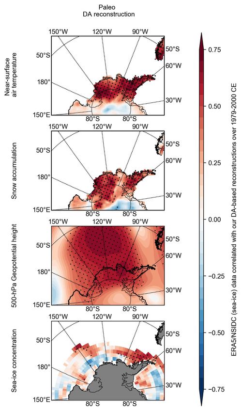
2                                                            Quentin Dalaiden et al.

15   assimilation method. This ultimately provides a complete spatial reconstruc-
16   tion over the West Antarctic region. Our reconstruction reproduces well the
17   main characteristics of the observed changes over the instrumental period. We
18   show that the observed sea-ice reduction in the Bellingshausen-Amundsen Sea
19   sector over the satellite era is part of a long-term trend, starting at around
20   1850 CE, while the sea-ice expansion in the Ross Sea sector has only started
21   around 1950 CE. Furthermore, according to our reconstruction, the Amundsen
22   Sea Low pressure (ASL) displays no significant linear trend in its strength or
23   position over 1850–1950 CE but becomes stronger and shifts eastward after-
24   wards. The year-to-year sea-ice variations in the Ross Sea sector are strongly
25   related to the ASL variability over the past two centuries, including the recent
26   trends. By contrast, the link between ASL and sea-ice in the Bellingshausen-
27   Amundsen Sea sector changes with time, being stronger in recent decades than
28   before. Our reconstruction also suggests that the continental response to the
29   variability of the ASL may not be stationary over time, being significantly
30   affected by modification of the mean circulation. Finally, we show that the
31   widespread warming since 1958 CE in West Antarctica is unusual in the con-
32   text of past 200 years and is explained by both the deeper ASL and the positive
33   phase of the Southern Annular Mode.
34   Keywords climate reconstruction · Antarctic · ice cores · climate models ·
35   data assimilation

36   1 Introduction

37   The Antarctic Ice Sheet is the biggest reservoir of fresh water on Earth that
38   would potentially raise the global sea-level by 58m if the entire ice sheet melted
39   (Shepherd et al., 2018). Despite the remote location, the Antarctic and the
40   Southern Ocean have experienced major climate changes over the past decades
41   (e.g., Jones et al., 2019; Bromwich et al., 2013; Medley and Thomas, 2019;
42   Pritchard et al., 2012), demonstrating large variability and their vulnerability
43   to the global climate change.
44       The largest changes have been found over the Antarctic Peninsula and the
45   West Antarctic Ice Sheet (hereafter WAIS) (e.g., Jones et al., 2019), together
46   forming West Antarctica. A major warming has been observed since the Inter-
47   national Geophysical Year (i.e., 1958 CE), far exceeding the global warming
48   during the same period (Vaughan et al., 2003; Turner et al., 2005a; Nicolas
49   and Bromwich, 2014). Although the warming is particularly pronounced over
50   the Peninsula, the warming over the central WAIS since the 1950s is one of the
51   fastest recorded on Earth (Steig et al., 2009; Bromwich et al., 2013). Moreover,
52   in the last decades, glaciers from West Antarctica (especially the Thwaites and
53   Pine Island glaciers) have been losing mass at the ocean-ice shelf (i.e., the float-
54   ing part of the glacier) interface at an accelerated rate (Pritchard et al., 2012;
55   Rignot et al., 2019). This ice shelf melting positively contributes to the global
56   sea-level rise, by directly enhancing the ice flow to the Southern Ocean. In con-
57   trast with these spatially homogeneous changes, snow accumulation integrated
West Antarctic Climate reconstruction over the past two centuries               3

 58   over West Antarctica has increased at an increased pace over the 20th century,
 59   but with strong regional differences (Medley and Thomas, 2019; Wang et al.,
 60   2019). While the Antarctic Peninsula and the Eastern WAIS have gained mass
 61   at the surface through snow accumulation, the Western WAIS has displayed a
 62   snow accumulation decrease (Medley and Thomas, 2019; Wang et al., 2019).
 63   Additionally, a large reduction of the sea-ice extent has been noticed in the
 64   Bellingshausen/Amundsen Sea sector that contrasts with an expansion in the
 65   Ross Sea sector over the satellite era (starting from 1979 CE) (Parkinson,
 66   2019).
 67       The observed changes in West Antarctica are not independent of each
 68   other, and have been widely attributed to changes in atmospheric circulation
 69   (e.g., Bromwich et al., 2013; Thomas et al., 2013; Steig et al., 2013), charac-
 70   terized by an increase in the intensity and a poleward shift of the westerly
 71   winds (Westerlies) (Marshall, 2003). This has been observed as a deepening
 72   in the Amundsen Sea Low (ASL), a quasi-stationary low-pressure system lo-
 73   cated off the Amundsen coast (hereafter ASL) (e.g., Raphael et al., 2016).
 74   Due to its location, variations in both the strength and position of the ASL
 75   strongly modulate the West Antarctic climate (e.g., Hosking et al., 2013). For
 76   instance, a stronger ASL enhances the northerly flow (onshore winds) to the
 77   continent, which warms the Antarctic Peninsula and the eastern WAIS (e.g.,
 78   Hosking et al., 2013) and increases snow accumulation (Turner et al., 2005b;
 79   Thomas et al., 2008). At the same time a stronger ASL enhances the southerly
 80   flow (offshore winds) of cold dry air masses over the western WAIS leading to
 81   lower temperatures and reduced snow accumulation. In addition to continen-
 82   tal changes, a stronger ASL is also associated with reduced sea-ice cover in
 83   the Bellingshausen/Amundsen Sea sector and a sea-ice cover expansion in the
 84   Ross Sea sector (e.g., Raphael and Hobbs, 2014). A deeper ASL also drives
 85   oceanic changes, enhancing warm ocean water upwelling towards ice shelves,
 86   inducing basal melting (e.g., Mankoff et al., 2012; Dotto et al., 2020).
 87       The ASL is thus a major feature of the atmospheric circulation in the
 88   Southern Hemisphere, which displays one of the greatest year-to-year varia-
 89   tions on Earth (e.g., Turner et al., 2019). The ASL is strongly modulated by
 90   the atmospheric circulation of the high latitudes of the Southern Hemisphere.
 91   Particularly, the Southern Annular Mode (hereafter SAM) describes the lat-
 92   itudinal movement of the Westerlies as well as their strength (e.g., Fogt and
 93   Marshall, 2020). When the SAM is in its positive phase, the Westerlies are
 94   stronger and located further south than in the negative phase, which in turn
 95   deepens the ASL (e.g., Raphael et al., 2016). The ASL is thus strongly related
 96   to the SAM. Wind changes in the West Antarctic are also closely linked to
 97   the climate variability in tropical oceanic basins. Several studies (e.g., Ding
 98   et al., 2011; Steig et al., 2013; Thomas et al., 2013; Meehl et al., 2016; Holland
 99   et al., 2019) have suggested the important tropical teleconnections that exist
100   between the mid-latitudes/tropics and the West Antarctic. More specifically,
101   positive anomalies in sea surface temperature in the tropical Pacific Ocean
102   induce a convective heat event that further propagates to the West Antarctic
103   region via the formation of Rossby wave train.
4                                                            Quentin Dalaiden et al.

104       Despite the large changes observed recently, the impact of the ASL vari-
105   ability on West Antarctic climate changes has not been fully studied because
106   in-situ observations are lacking (Turner et al., 2004). Over the satellite era
107   (from 1979 CE), atmospheric reanalyses seem to be reliable for studying the
108   ASL variability and its impacts on the West Antarctic climate (Bracegirdle,
109   2013). However, because of the high internal variability in the Amundsen re-
110   gion (e.g., Raphael et al., 2016), longer time-series are needed to understand
111   the processes controlling the variability in the region.
112       In this study, we aim to better understand the West Antarctic climate
113   variability on decadal to centennial timescales by analyzing the relationships
114   between the main atmospheric variables with surface conditions and sea-ice
115   cover. Furthermore, by making use of those potential links between variables,
116   we provide historical estimations over the past two centuries that could not be
117   directly observed. Special attention is given to the ASL, because of its major
118   importance in the ongoing observed changes in West Antarctica. We investi-
119   gate to which extent the ASL variability explains the West Antarctic climate
120   change over the past two centuries, and if the role of the ASL has changed
121   over time. The sea-ice extent (in particular the Bellingshausen/Amundsen Sea
122   and Ross Sea sector) is also examined due to its key role in modulating West
123   Antarctic climate (e.g., Lefebvre and Goosse, 2008; Thomas et al., 2013; Turner
124   et al., 2017). Up to now, no spatial estimate of wind fields or sea-ice extent has
125   been specifically validated for this region before the instrumental era and thus
126   we aim to fill this gap. In addition to improving the general long-term changes
127   in the West Antarctic climate, we assess the representativeness of the climate
128   changes occurring during the second half of the 20th century on a longer time
129   perspective. Finally, a complementary goal is to highlight the mechanisms that
130   explain the warming over West Antarctica as a whole and the strong regional
131   asymmetry in sea-ice extent trends over the past decades.
132       To this end, we provide a spatially complete and multi-variate reconstruc-
133   tion of the West Antarctic climate changes over the past two centuries (the pe-
134   riod for which most paleoclimate proxies are available; see below) by optimally
135   combining paleoclimate records and a climate model using a data assimilation
136   approach. Over last years, data assimilation has been increasingly applied in
137   paleoclimatology for estimating past climate changes (e.g., Goosse et al., 2009;
138   Hakim et al., 2016; Steiger et al., 2017; Goosse et al., 2010). Compared to sim-
139   pler statistical methods (e.g., Stenni et al., 2017; Emile-Geay et al., 2017), data
140   assimilation does not assume a stationary relationship between the proxy and
141   the climate. Data assimilation ensures that the resulting climate reconstruc-
142   tion is dynamically coherent. Such a method is also particularly relevant for
143   regions like the West Antarctic where a strong coupling exists between the
144   observed changes from various variables (Jones et al., 2016; Fan et al., 2014;
145   Goosse et al., 2009). Here, the model is constrained by δ 18 O and snow ac-
146   cumulation records from Antarctic ice cores. Over the Antarctic, ice core is
147   the most widespread climate archive for assessing historical climate changes
148   at high temporal resolution (i.e., annual scale). Compared to the instrumental
149   network, the ice core network is well developed over West Antarctica thanks
West Antarctic Climate reconstruction over the past two centuries                5

150   to a number of international drilling efforts. In addition to the ice cores, we
151   also make use of the tree-ring width records from the mid-latitudes that cap-
152   ture changes in past climate variability (e.g., Emile-Geay et al., 2017). The
153   inclusion of non-specific-Antarctic proxies guarantees a large-scale coherence.
154   This avoids forcing a local agreement with the Antarctic data that would not
155   be based on processes compatible with larger-scale changes.
156       This study is organized as follows. Section 2 includes a description of the
157   data assimilation method, the paleoclimate proxies and the model used for the
158   reconstruction. We discuss the performance of our reconstruction in section 3
159   by comparing it with instrumental observations and other climate reconstruc-
160   tions, and discuss our main results, before concluding.

161   2 Data assimilation method

162   Data assimilation (DA) optimally combines the information from observations
163   and the climate physics as included in climate models. In practice, the data as-
164   similation process updates the initial state of the climate given by the model
165   (i.e., the prior) according to the available observations to provide the best
166   estimate of the climate state (i.e., the posterior), while also considering the er-
167   rors associated with both the data and model. Paleo DA methods thus spread
168   the local and temporal information from proxy records in space but also into
169   other variables by relying on the modelled co-variance in space and among
170   variables, respectively. For instance, the 500-hPa geopotential height can be
171   therefore reconstructed only by assimilating near-surface air temperature. In
172   that situation, the reconstructed 500-hPa geopotential height relies on the
173   covariance relationships between the 500-hPa geopotential height and near-
174   surface air temperature in the model. If there is no covariance between the
175   variable of interest and the assimilated variable, the reconstruction skill of the
176   variable of interest will be null. Consequently, the resulting multi-variate cli-
177   mate reconstruction guarantees a dynamical consistency in space and between
178   variables, which is provided in a natural way with the climate model as it
179   directly relies on the physics included in the climate model.
180       The DA method employed in this study is an offline approach (also called
181   a no-cycling method). This method uses existing climate model simulations to
182   draw the prior. In contrast to the standard online data assimilation approach,
183   the prior is estimated by selecting different years of a climate model simula-
184   tion. Therefore, no information is propagated in time. This approach is totally
185   appropriate when the predictability time-scale of the system is much smaller
186   than the data assimilation time step (here, one year). This is particularly true
187   when assimilating atmospheric variables because of the small correlation time
188   in the atmosphere. In such cases, no additional relevant information is gained
189   when using an online approach, as shown by Matsikaris et al. (2015).
6                                                                Quentin Dalaiden et al.

190   2.1 Particle filter

191   The DA method used here is based on a particle filter following the imple-
192   mentation of Dubinkina et al. (2011). This method has been recently applied
193   to reconstruct successfully large-scale near-surface air temperature and snow
194   accumulation over Antarctica during the past millennia (Klein et al., 2019;
195   Dalaiden et al., 2020a). We thus describe briefly the method here.
196       The particle filter (van Leeuwen, 2009) aims at updating an initial esti-
197   mate of the state of the system, referred to as the prior, using additional infor-
198   mation provided by available observations, following the classical approach of
199   Bayesian reconstructions. Specifically, the prior for each variable is represented
200   by a probability density function (pdf), described in a discrete way using a set
201   of independent model states, which are called particles. These model states
202   are given by all the years (annual mean) of an ensemble of three simulations
203   performed with the isotope-enabled Community Earth System Model version
204   1 (iCESM1; Brady et al., 2019; Stevenson et al., 2019) spanning the 850–1850
205   CE period (see section 2.5 for the model evaluation). The prior thus includes
206   3003 particles and is constant throughout the data assimilation process. At
207   each assimilation step (here every year), the particles forming the prior are
208   evaluated against the available observations while taking into account the er-
209   ror associated with the observations as well as the inconsistency between the
210   observations and model related to unresolved processes in the model (i.e., the
211   observation error; see section 2.6). As a result of this comparison with obser-
212   vations, each particle of the prior receives a weight that is proportional to its
213   likelihood knowing the observations. The weights are thus higher for the parti-
214   cles closer to the observations than for the particles further to the observations.
215   In other words, the particle filter redistributes the weights of all the particles
216   at each time step to obtain posterior distribution in better agreement with
217   observations. Since only the weights of the particles can change during the
218   data assimilation process, the climate dynamics as represented in the model is
219   fully respected. For each time step, the climate reconstruction is defined as the
220   weighted mean of all the particles. We define the reconstruction uncertainty
221   as the weighted standard deviation of all the particles. For more details on the
222   implementation of the particle filter, see Dubinkina et al. (2011).

223   2.2 Evaluation metrics

224   In order to quantify the performance of our reconstruction, we use three dif-
225   ferent metrics that compare the results with observations or other reconstruc-
226   tions. The first one is the Pearson correlation coefficient (r ), which determines
227   the strength of the linear relationship between two time-series:

                                       n
                                    1X          (yi − y)(xi − x)
                               r=                                                         (1)
                                    n i=1             σy σx
West Antarctic Climate reconstruction over the past two centuries                 7

228   where n is the number of samples, y stands for the predicted vector while
229   x is the true vector. Overbars indicate the mean over the time. σy and σx
230   are the standard deviations of y and x, respectively. Although a high value of
231   r indicates that the predicted values follow the direction of the true values,
232   it does not ensure that the variations of the amplitude are well reproduced.
233   Therefore, the second metric is the coefficient of efficiency (Nash and Sutcliffe,
234   1970), which depends on the amplitude of the signal:
                                                n
                                                X (xi − yi )2
                                    CE = 1 −                                          (2)
                                                i=1
                                                      (xi − x)2
235   A high value for CE thus indicates that both the timing and the amplitude
236   are right. Finally, we need to verify if the ensemble reconstruction is similar to
237   the reconstruction error relative to observations. For this purpose, we compute
238   the ensemble calibration ratio (ECR) defined here as:
                                                  "             #
                                                    (xi − yi )2
                                ECR = median            2                            (3)
                                                       σx,i
                                           2
239   where i varies from 0 to n and σx,i     is the variance of the reconstruction
240   ensemble. An ECR of 1 means that the reconstruction is well calibrated
241   (i.e., the reconstruction error equals the uncertainty of the reconstruction).
242   When ECR1, the estimate of the uncertainty is likely too low compared to the real
245   reconstruction error.

246   2.3 Proxy data

247   From the 79 ice core snow accumulation records included in the database of
248   Thomas et al. (2017), we only keep the annually-resolved records (48 out of
249   79) as in Medley and Thomas (2019). Medley and Thomas (2019) provide a
250   spatially complete annual Antarctic snow accumulation over the past two cen-
251   turies using this ice core snow accumulation database (Fig. 1). This excludes
252   a majority of snow accumulation records in the continental Dronning Maud
253   Land region. As in Medley and Thomas (2019), we also add the B40 ice core
254   record of snow accumulation (Medley et al., 2018), which was published after
255   the compilation of Thomas et al. (2017). Additionally, we also employ the infor-
256   mation from the ratio of stable isotopes oxygen in the ice core (δ 18 O). Stenni
257   et al. (2017) provide a compilation of the Antarctic precipitation-weighted
258   δ 18 O records (n=112) covering the last two millennia. We only keep the 29
259   annually-resolved δ 18 O records. It is worth noting that the majority of the ice
260   cores (both snow accumulation and δ 18 O records) are located in West Antarc-
261   tica (WAIS; Fig. 1).
262        In addition to the Antarctic proxies, we also utilize the continental annually-
263   resolved proxies situated in the Southern Hemisphere from the global database
8                                                                                          Quentin Dalaiden et al.

                          Snow accumulation records (n=48)                              18   O records (n=29)
                                          0°                                                         0°

              90°W                                            90°E     90°W                                                    90°E

                                         180°                                                    180°
                           Tree Ring Width records (n=12)                                    AWS (n=14)
                                          0°                                                         0°

              90°W                                            90°E     90°W                                                    90°E

                                         180°                                                    180°

          0          50      100   200     300   500    750    1000 1250      1500   1750     2000        2500   3000   4000
                                                              Elevation [m]

      Fig. 1 Annually-resolved climate/proxy records used in this study: snow accumulation
      records (blue dots), δ 18 O records (purple squares), Automatic Weather Stations (AWSs;
      green stars) and tree-ring width records (green dots). The map background represents the
      surface elevation (m).

264   of the PAGES2k working group that includes all the proxy records suitable for
265   reconstructing the global temperature over the last two millennia (PAGES2k
266   Consortium et al., 2013; Emile-Geay et al., 2017). Among all the continental
267   proxies included in the global database for the Southern Hemisphere, only the
268   tree-ring width (hereafter TRW) are annually-resolved (in addition to some
269   Antarctic ice cores already included in our study). A total of 18 sites present-
270   ing TRW time-series over past centuries are located in the Southern Hemi-
271   sphere : three in New Zealand, three in Tasmania and 12 in South America.
272   Among the 12 South American sites, only six are positively correlated with
273   climate (either near-surface air temperature or precipitation) according to our
West Antarctic Climate reconstruction over the past two centuries              9

274   dataset (see section 2.4) over the 1941–1990 CE period, and thus included.
275   The geographical distribution of the selected sites is presented in Fig. 1.
276       Most proxy records cover the last two centuries, but their number starts
277   to decline from around 1990 CE (Fig. S1). Therefore, the period analyzed
278   throughout the study is 1800–2000 CE. This provides a good compromise
279   in terms of the number of records and the overlap with the satellite period
280   (starting in 1979 CE) that is used for the evaluation of the reconstruction (see
281   section 3.1). This period was also used in the study of Medley and Thomas
282   (2019) who reconstructed snow accumulation in Antarctica using the same ice
283   core snow accumulation records as here.
284       In order to reduce the non-climatic noise and provide equal weighting in
285   each region (i.e not bias a particular region with multiple records), a 500
286   km grid (square cells of 500 km side) was established and records from the
287   same grid were averaged together. For snow accumulation records, they are
288   all normalized over the 1941–1990 CE period (mean zero and unit standard
289   deviation) and the records situated in the same cell are averaged. The mean
290   of normalized snow accumulation records for each grid cell produces the nor-
291   malized composites. For each composite, the variance is then scaled to the
292   variance of the spatial snow accumulation reconstruction from Medley and
293   Thomas (2019), linearly interpolated on the 500 km grid over the 1941–1990
294   CE period. Compared to snow accumulation, the δ 18 O records display a weaker
295   spatial variability as they are less dependent on the topography and do not
296   need normalization. Instead, δ 18 O composites for each grid cell are obtained
297   by averaging the anomalies of δ 18 O records over the 1941–1990 CE. Finally, we
298   apply the same methodology as for the snow accumulation records to TRW
299   time-series, but without correcting the variance (z-scored composites) since
300   TRW data is originally normalized.

301   2.4 Proxy System Models

302   Snow accumulation records are directly compared to the precipitation minus
303   sublimation/evaporation (P − E) from the climate model simulation. Snow
304   accumulation recorded in ice cores is the sum of both precipitation and post
305   depositional changes (wind erosion, sublimation and melt). Several studies
306   have shown that precipitation dominates and that snow accumulation can
307   be directly compared with the precipitation minus sublimation/evaporation
308   (P − E) from the climate model simulation (Lenaerts et al., 2017; Souverijns
309   et al., 2018; van Wessem et al., 2018; Agosta et al., 2019). This is particularly
310   true when working at a large spatial scale – as in our study (500 km grid)
311   – and over the grounded ice sheet (i.e., the Antarctic Ice Sheet without ice
312   shelves) (Agosta et al., 2019). Additionally, since iCESM1 explicitly simulates
313   the ratios of water isotopes in all the climate components, the δ 18 O records
314   are also directly compared to the δ 18 O simulated by the model.
315       A Proxy System Model (PSM) specifically designed for the TRW is required
316   in order to compare the model results to the proxy. To this end, a TRW
10                                                          Quentin Dalaiden et al.

317   PSM is built for each TRW time-series. Instead of a mechanistic model, which
318   simulates tree-ring growth by explicitly including the biological processes that
319   drives the relationship between climate and tree growth (e.g., Guiot et al.,
320   2014; Misson, 2004; Dufrêne et al., 2005; Rezsöhazy et al., 2020), we use a
321   simple statistical model. It has the advantage of being easily implemented
322   but the relationship between climate and tree growth is estimated empirically,
323   without taking into account any biological processes. This method is similar
324   to the one used in the Last Millennium Reanalysis (Tardif et al., 2019).
325       In this study, we consider that trees are sensitive to the temperature or
326   precipitation, or to both. Therefore, we introduce two types of models:

                                   yi = β0i + β1i X1i + ǫi                           (4)

                              yi = β0i + β1i X1i + β2i X2i + ǫi                      (5)
327   where yi corresponds to the observed z-scored TRW time-series (i.e., the de-
328   pendent variable) for site i ; β1i and β2i are the slopes associated with the X1i
329   and X2i of the i time-series, which are the explanatory variables; ǫi are the
330   errors, assumed to be normally (Gaussian) distributed with a zero mean and
331   a unitary variance (0, σ 2 ). Parameters of the Eqs. (4) and (5) are estimated
332   using the ordinary least squares method.
333       Similarly to the Last Millennium Reanalysis (Tardif et al., 2019), we use
334   the near-surface air temperature and precipitation as explanatory variables
335   (X1 and X2 ). In addition to the annual mean of near-surface air temperature
336   and precipitation, the climate variables are also averaged over different months
337   during the calendar year (January to December), in order to take into account
338   the seasonal response of trees: JJA and OND. All the possible combinations
339   are tested. The calibration of the PSM is performed over the 1941–1990 CE
340   period using the Global Meteorological Forcing Dataset for land surface mod-
341   eling (v2; http://hydrology.princeton.edu/data.php, last access: 22 June 2020;
342   hereafter GMF) (Sheffield et al., 2006) interpolated on the 500 km grid ex-
343   cluding the oceanic grid cells. The sensitivity to the climate data has been
344   assessed by also performing the calibration with the surface temperature from
345   the NASA Goddard Institute for Space Studies Surface Temperature Analysis
346   (Hansen et al., 2010) and precipitation from the Global Precipitation Clima-
347   tology Centre (Schneider et al., 2014). Results display no major difference (not
348   shown).
349       To select the best PSM for each TRW composite, we rely on the Bayesian
350   information criterion (BIC) (Schwarz, 1978) value defined as :

                               BIC = −2 ∗ LL + log(n) ∗ k                            (6)
351   where LL is the natural logarithm of the likelihood for the model – estimated as
352   the mean squared error of the linear regression model (Watkins and Mardia,
353   1992) – and k corresponds to the number of parameters in the regression
354   model (i.e., 2 and 3 for the uni and bi-variate models, respectively). The BIC
West Antarctic Climate reconstruction over the past two centuries 11 355 is a particularly relevant metric to select the best model among uni and bi- 356 variate models as the most complex models are penalized. Accordingly, the 357 PSM displaying the lowest BIC is selected. 358 2.5 Climate model simulation 359 The initial estimate of the state of the climate system (i.e., the prior) is derived 360 from an ensemble of three simulations performed with the isotope-enabled 361 iCESM1 spanning the 850–1850 CE time period (Brady et al., 2019; Stevenson 362 et al., 2019). iCESM1 is a coupled atmosphere-ocean model including a sea-ice 363 component. The atmosphere is resolved at approximately 2◦ and the ocean at 364 1◦ . The iCESM1 simulations include the orbital changes, the solar variability, 365 the volcanic forcing through changes in stratospheric aerosols and greenhouse 366 gases, the land use changes and finally the human-induced greenhouse gases 367 (Stevenson et al., 2019). 368 Although numerous studies have shown that CESM is well-suitable for 369 studying the Antarctic climate over the past, present and future (Lenaerts 370 et al., 2016; Fyke et al., 2017; England et al., 2016; Lenaerts et al., 2018; 371 Dalaiden et al., 2020b), this version has not yet been evaluated over the 372 Antarctic continent. As the information from proxy records is spread spa- 373 tially and into other variables using the climate model, it is important to 374 assess the performance of the model used in the data assimilation in simulat- 375 ing the near-surface climate over the Antarctic. Therefore, we briefly evaluate 376 the Antarctic climate as simulated by iCESM1 by comparing it to the latest 377 ECMWF’s atmospheric reanalysis, ERA5 (Hersbach et al., 2020). It is consid- 378 ered as one of the best reanalyses in simulating the Antarctic climate over the 379 satellite-era (Gossart et al., 2019; Tetzner et al., 2019). Since the paleoclimate 380 proxies used in this study are annually-resolved, the evaluation is carried out 381 on annual averages. 382 Over the 1979–2005 CE period, the geopotential height at 500-hPa is 383 well simulated in iCESM1 (Fig. S2; below south of 45◦ S, R2 =97%; relative 384 bias=-0.2% computed as the mean relative difference between the 500-hPa 385 geopotential height from iCESM1 and ERA5 south of 45◦ S) and includes the 386 three main low-pressure systems in Amundsen Sea, Dronning Maud Land and 387 Wilkes Land. Regarding the near-surface air temperature, iCESM1 simulates 388 the temperature gradient with the highest temperatures along the coasts and 389 the lowest temperatures in the interior of the ice sheet (over the Antarctic 390 continent, R2 =76%; relative bias=-2.0%). Like temperature, snow accumula- 391 tion is highly dependent on the topography. iCESM1 reproduces the Antarctic 392 snow accumulation pattern well from ERA5 (R2 =85% – based on log values 393 as the snow accumulation distribution is log-normal (Agosta et al., 2019)– 394 ; relative bias=-6.9%). However, iCESM1 is not able to reproduce the high 395 spatial variability of snow accumulation at local scale, because of its coarse 396 horizontal spatial resolution. Besides, iCESM1 displays a total Antarctic sea- 397 ice extent of 11.7 106 km2 against 11.9 106 km2 for observations from the
12                                                            Quentin Dalaiden et al.

398   National Snow and Ice Data Center (NSIDC; data available here: https:
399   //nsidc.org/data/NSIDC-0051/versions/1, last access: 5 September 2018).
400   Compared with the NSIDC observations, iCESM1 overestimates by 5% the
401   mean sea-ice extent in the West Antarctic sector (160◦ W-60◦ E) over 1979–2005
402   CE, with a similar bias in both the Bellingshausen/Amundsen Sea (130◦ W-
403   60◦ E) and Ross Sea (160◦ E-130◦ W) sectors (5.4% and 4.8%, respectively; Tab.
404   S1). This suggests that iCESM1 is able to simulate relatively well the mean
405   state of Antarctic sea-ice extent at present. Finally, although a quantitative
406   evaluation of the simulated precipitation-weighted δ 18 O is not possible be-
407   cause of the insufficient amount of Antarctic observations (three records in
408   the Global Network of Isotopes in Precipitation), the precipitation-weighted
409   δ 18 O pattern over Antarctica captures the gradient between the coasts (with
410   the highest values, less negative) and the Plateau (with the lowest values, more
411   negative) due to isotopic fractionations (Fig. S3). Based on the skill of iCESM1
412   in simulating present-day Antarctic climate, we deem this model suitable for
413   building the prior of the data assimilation experiment. As proxy data are av-
414   eraged over a 500 km regular grid (see section 2.3), the prior has also been
415   linearly interpolated onto this 500km regular grid.

416   2.6 Observation error

417   Data assimilation requires an error of the assimilated data. This observation
418   error plays a crucial role in data assimilation because it determines the ex-
419   tent to which each assimilated record is influencing the reconstruction. The
420   records with a low observation error will thus have a larger weight in the data
421   assimilation than the records with a high observation error.
422       Three types of observation errors are usually mentioned (e.g., Badgeley
423   et al., 2020). The first type of observation error directly comes from the ac-
424   curacy of the measurement, i.e., the instrumental error. The second type of
425   observation error is related to the processes in observations that are unresolved
426   at the spatial scale of the model because of its coarse resolution , the so-called
427   representativeness observation error (e.g., Oke and Sakov, 2008; Janjić et al.,
428   2018). Finally, the last type of observation error arises from the performance
429   of the PSM in simulating the relationship between the proxy and the climate
430   variable(s). Overall, the instrumental error is much smaller than the two other
431   observation errors (e.g., Oke and Sakov, 2008), especially in paleoclimatology
432   (Tardif et al., 2019; Steiger et al., 2018; Badgeley et al., 2020). This observation
433   error is thus ignored in our study. Finally, regarding the snow accumulation
434   and δ 18 O records, we assume that the observation error related to the PSM
435   is non-existent, since the model simulates both variables. The representative-
436   ness error is thus considered as the largest contributor to the observation error.
437   Therefore, for ice core snow accumulation and δ 18 O records, the observation er-
438   ror is taken equal to the representativeness error. However, for tree-ring width
439   records, the observation error combines the representativeness error and the
440   PSM-related observation error as the climate model used in the data assimi-
West Antarctic Climate reconstruction over the past two centuries             13

441   lation does not simulate tree growth. In contrast, the climate model simulates
442   the snow accumulation and δ 18 O. As a consequence, a PSM simulating those
443   variables is not required.
444       To estimate the representativeness error of the snow accumulation com-
445   posite associated with the ice core records, we use an Antarctic simulation
446   performed with the latest version of the Regional Atmospheric Climate MOdel
447   (RACMO2.3p2, hereafter RACMO) at 27 km horizontal resolution (van Wessem
448   et al., 2018). RACMO is a polar-oriented regional climate model that specif-
449   ically resolves near-surface processes over Antarctica. For each snow accumu-
450   lation composite, we proceed as follows. We retrieve the annual time-series
451   of snow accumulation from RACMO at the location of all the ice core snow
452   accumulation records included in the composite over the 1979–2016 CE pe-
453   riod (period over which RACMO results are available). In order to remove
454   the dependence on the elevation, the calculation is performed on time-series
455   anomalies. All RACMO-time series are then averaged in time. Next, we com-
456   pute the difference between this averaged snow accumulation time-series and
457   the snow accumulation time-series from RACMO interpolated on the 500 km
458   grid (i.e., the resolution of snow accumulation composites; see section 2.3).
459   Eventually, the representativeness error is defined as the standard deviation
460   of the time-series difference. Note that the representativeness error is calcu-
461   lated for each year of the composite (1800–2000 CE), based on the snow ac-
462   cumulation RACMO data (1979-2016 CE). As the number of ice cores in the
463   composite decreases when going further back in time, the representativeness
464   error tends to increase. Finally, since RACMO does not simulate the δ 18 O,
465   we use the iCESM1 linearly interpolated on the RACMO grid over the 1950–
466   2005 CE period to estimate the δ 18 O representativeness error with the same
467   methodology. A 50-year period minimizes the potential biases induced by the
468   variability of the δ 18 O when using a too short time period and thus ensures the
469   computation of a robust estimate. We have selected the final part of the series
470   to have the largest overlap with the period over which the snow accumulation
471   error is computed. This in part guarantees consistency in the calculation of
472   the representativeness error for the snow accumulation and δ 18 O records.
473       However, several studies (van Wessem et al., 2018; Lenaerts et al., 2016;
474   Cavitte et al., 2020) have shown that the spatial variability of snow accumula-
475   tion and δ 18 O is underestimated in models (i.e., RACMO and iCESM1) com-
476   pared to ice core observations. Therefore, using these models to estimate the
477   observation error in our study probably also underestimates the observation
478   errors. In order to provide an observation error closer to the reality, we take
479   into account the missing processes occurring between the scale represented in
480   the models and the local scale of ice cores. This is achieved by performing
481   a side-by-side comparison between adjacent snow accumulation records as in
482   Fisher et al. (1985). More specifically, we compute the standard deviation of
483   the difference between each pair of annual time-series of snow accumulation
484   records (in anomalies) within the same grid cell of the 500 km grid over the
485   1941–1990 CE (which is the most recent 50-year period for which all the ice
486   core records are available; Fig. S1). The calculation is made for all the possible
14                                                         Quentin Dalaiden et al.

487   combinations within the grid cell. According to the grid cell containing more
488   than five ice cores (n=2; both situated in West Antarctica), the side-by-side
489   comparison suggests that the error at the ice core-scale is higher by a three-
490   factor compared to the one at the scale of RACMO. The same exercise for
491   δ 18 O has been carried out and shows similar results (not shown).
492        Regarding the TRW composites, the error is estimated by taking the stan-
493   dard deviation of the residuals resulting from the linear regression (see Eqs.
494   (4) and (5)) as in the Last Millennium Reanalysis (LMR) (Hakim et al., 2016;
495   Tardif et al., 2019). The error thus encompasses the representativeness error
496   and the error related to the PSM since the PSM has been calibrated using
497   the climate data interpolated on the 500 km grid and not using the local
498   data. After performing several sensitivity tests, we have found that our results
499   present a small sensitivity to reasonable modification of the estimation of the
500   observation error (not shown).

501   2.7 Instrumental data assimilation-based reconstruction

502   Before using the paleo records to reconstruct the Antarctic climate over the
503   past centuries (hereafter referred to as the paleo-reconstruction), we first re-
504   construct the Antarctic climate over the 1958–2000 CE period using data as-
505   similation with near-surface air temperature records and snow accumulation
506   records from ice cores. Applying a methodology that is as close as possible to
507   the one selected for the longer timescales allows us to validate the approach,
508   in particular the data assimilation method and the estimations of the errors
509   using observations with lower uncertainties than the paleo records. This recon-
510   struction based on instrumental and snow accumulation records thus provides
511   an upper bound for the skill we could expect with the paleoclimate network.
512   To this end, we assimilate the near-surface air temperatures from the Auto-
513   matic Weather Stations (AWSs) over the Antarctic continent (Turner et al.,
514   2004) (n=14) starting from 1958 CE (see Fig. 1 for their geographical localiza-
515   tion). The model is also constrained by the snow accumulation records from
516   ice cores, which are the best estimate of long-term snow accumulation, since
517   AWSs do not record this variable. Additionally, TRW records are replaced by
518   the near-surface air temperatures from the gridded dataset used for the cal-
519   ibration of the TRW PSM (i.e., GMF; only where TRW sites are available).
520   This reconstruction is referred to as the instrumental reconstruction.
521       The observation error on the near-surface air temperature from AWSs is
522   calculated similarly to the snow accumulation error (see section 2.6) but using
523   near-surface air temperatures from RACMO. Like for the snow accumulation
524   and δ 18 O records, we assume that the observation error for the Antarctic
525   near-surface air temperature is mainly due to the representativeness error.
526   This error should take into account the missing processes occurring between
527   the local scale (i.e., the AWS scale) and the scale of RACMO (i.e., 27-km
528   resolution). Nevertheless, the network of AWS starting from 1958 CE is much
529   less dense than the paleo records (Fig. 1). Therefore, a side-by-side comparison
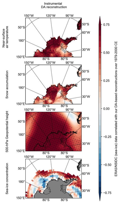
West Antarctic Climate reconstruction over the past two centuries              15

530   of adjacent near-surface air temperature time-series as we did for paleo records
531   is not possible (see section 2.6). We are thus not able to provide an accurate
532   estimate of the factor to make the link between local observation error and
533   the error at the scale on the climate model grid. However, several studies
534   (e.g., Agosta et al., 2019; van Wessem et al., 2018) showed a weaker spatial
535   variability of near-surface air temperature compared to snow accumulation
536   (e.g., Agosta et al., 2019; van Wessem et al., 2018). Therefore, we assume that
537   the factor applied to take into account the unresolved processes at the RACMO
538   scale is smaller than for snow accumulation (see section 2.6) and multiply the
539   local observation error of near-surface air temperature for the Antarctic AWSs
540   by a two-factor. Finally, the situation is very different for the assimilated near-
541   surface air temperature of the gridded dataset GMF associated with the TRW
542   sites as it is a gridded dataset at a resolution similar to the one of the model
543   that is thus expected to represent processes at a similar scale. Therefore, a
544   constant error of 0.5 ◦ C is chosen, which is a typical value when assimilating
545   gridded near-surface air temperature (e.g., Brennan et al., 2020; Dubinkina
546   et al., 2011).

547   3 Results and discussion

548   3.1 Validation of the instrumental paleo reconstructions over the last decades

549   Before analyzing the long-term changes using the paleo-reconstruction over
550   the past centuries, we first need to ensure that our data assimilation method
551   works. We establish this by testing the skill of the instrumental and paleo
552   reconstructions at reproducing interannual climate variability and trends over
553   the last decades, in particular the atmospheric circulation, near-surface con-
554   tinental climate (temperature and snow accumulation) and sea-ice cover. To
555   this end, Figure 2 presents the spatial correlation coefficients between our
556   instrumental and paleo reconstructions and the latest ECMWF atmospheric
557   reanalysis ERA5 (Hersbach et al., 2020) over the 1979–2000 CE period for the
558   500-hPa geopotential height, near-surface air temperature and snow accumu-
559   lation, as well as sea-ice concentration using the dataset from the National
560   Snow and Ice Data Center (NSIDC) (Parkinson, 2019). Although the period
561   is short (22 years), this evaluation gives a first indication of the performance
562   of our reconstruction when compared to independent data.

563   3.1.1 Near-surface air temperature

564   For continental near-surface air temperature, our spatial instrumental recon-
565   struction is highly correlated with ERA5 over West Antarctica (Fig. 2). Our
566   instrumental reconstruction is also close to the reconstruction of Nicolas and
567   Bromwich (2014) – which is based on the same near-surface air temperature
568   observations as in our reconstruction but using a kriging interpolation over
16                                                          Quentin Dalaiden et al.

569   1958–2000 CE –, when averaging over the two main regions of the West Antarc-
570   tic continent, i.e., the West Antarctic Ice Sheet (WAIS; 60-180◦ E and south of
571   72◦ S; r =0.88 (p-value
West Antarctic Climate reconstruction over the past two centuries                         17

      Fig. 2 Spatial correlation coefficients (r) between our instrumental (left) and paleo (right)
      reconstructions and the ERA5 reanalysis for the near-surface air temperature, snow accu-
      mulation, 500-hPa geopotential height and the sea-ice concentration from the National Snow
      and Ice Data Center (NSIDC) over the 1979–2000 CE period. Stippling indicates statistically
      significant correlations (95% confidence level).

613   is particularly prevalent for regions in East Antarctica (Medley and Thomas,
614   2019). Since these snow accumulation records are used in our data assimilation,
615   it is not surprising to obtain lower correlation coefficients for those areas.
616        When evaluating our snow accumulation reconstruction compared to the
617   snow accumulation reconstruction from Medley and Thomas (2019), the skill
618   metrics show that our instrumental reconstruction displays good and similar
619   performance for the WAIS (r =0.64 (p-value
18 Quentin Dalaiden et al.
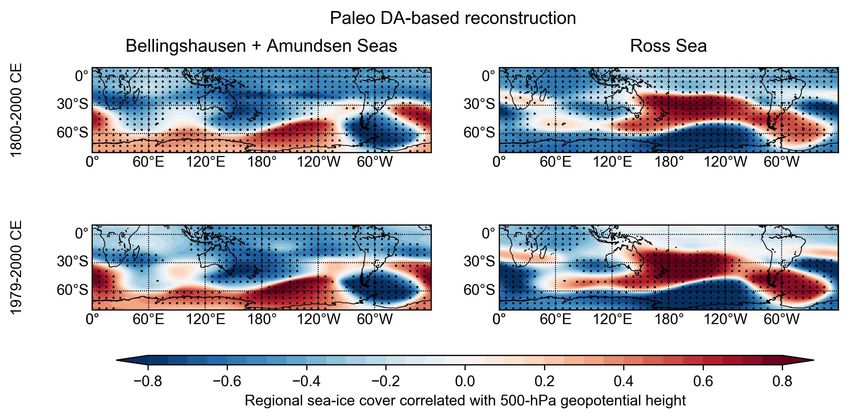
a. b.
c. d.
Fig. 3 (a-b) Comparison between our instrumental (red) and paleo (blue) near-surface air
temperature (SAT; ◦ C) anomalies and the reconstruction of Nicolas and Bromwich (2014;
NB2014; in black) for the West Antarctic Ice Sheet (WAIS; 60-180◦ E and south of 72◦ S)
and the Antarctic Peninsula (AP; west longitude north of 72◦ S) and over the 1958–2000
CE period. Regional definitions are identical as in Steig et al. (2009). (c-d) Comparison
between our instrumental (red) and paleo (blue) snow accumulation (Gt year-1 ; in red)
anomalies and the reconstruction of Medley and Thomas (2019; MT2019; in black) for the
West Antarctic Ice Sheet (WAIS) and the Antarctic Peninsula (AP) and over the 1958–
2000 CE period. Anomalies are computed over the 1958–2000 CE period. Linear trends
of near-surface air temperature trends and snow accumulation are displayed (expressed
in ◦ C decade -1 and Gt year-1 decade -1 , respectively) and the standard deviation (std)
of the time-series (expressed in ◦ C and Gt year-1 , respectively) over the 1958–2000 CE
period for each region. Asterisks indicate statistically significant trends at the 95% confidence
level. Additionally, the correlation coefficient (r), coefficient of efficiency (CE) and ensemble
calibration ratio (ECR) are computed over the 1958–2000 CE period. Error bands correspond
to the reconstruction uncertainty as defined in section 2.1.
623 accumulation (i.e., the sum of the WAIS and AP regions) over the 1958–2000
624 CE period: 18.48 Gt year-1 per decade and 11.46 Gt year-1 per decade, re-
625 spectively (both statistically significant; p-valueWest Antarctic Climate reconstruction over the past two centuries 19 637 year-1 per decade linear trend for the West Antarctic-wide snow accumulation 638 over 1958-2000 CE, which is very close to Medley and Thomas (2019) (18.48 639 Gt year-1 per decade over the same period). 640 3.1.3 Atmospheric circulation 641 Unlike near-surface air temperature and snow accumulation, no pressure data 642 is used in the data assimilation process for both the instrumental and paleo re- 643 constructions. The skill of the reconstruction of the non-assimilated variables is 644 thus expected to be lower than for the assimilated variables. Spatial correlation 645 coefficients between our instrumental reconstruction and the ERA5 reanaly- 646 sis for the 500-hPa geopotential height during the 1979–2000 CE period show 647 that interannual changes in the atmospheric circulation are well reconstructed 648 over the West Antarctic and in the mid-high latitudes of the Pacific Sector of 649 the Southern Hemisphere (Fig. 2). Furthermore, for the paleo-reconstruction, 650 the stronger correlations over the ocean, compared to the continent, reflect 651 the fact that changes in this region are driving the variability recorded in ice 652 cores. This confirms that marine intrusions predominantly govern the near- 653 surface climate variability in West Antarctica (Nicolas and Bromwich, 2011). 654 This also gives confidence in the use of ice core records for reconstructing the 655 atmospheric circulation in that sector. 656 We also analyze the Amundsen Sea Low pressure (ASL), which can be 657 characterized by several indexes (e.g., Hosking et al., 2013), for example related 658 to the change in the ASL position (latitudinal and longitudinal positions) or 659 to the intensity of the minimum pressure in the ASL region. Here, the ASL 660 index is defined as the annual average of the 500-hPa geopotential height from 661 75◦ S to 60◦ S and from 170◦ E to 70◦ W (Fogt et al., 2012; Turner et al., 2013; 662 Hosking et al., 2013). Note that geographical definitions can differ between 663 studies but the resulting indexes are relatively similar. This index is then 664 normalized (zero mean and unity standard deviation) over the 1941–1990 CE 665 period. Following this definition, a negative (positive) ASL index corresponds 666 to a deeper/stronger (weaker) ASL. Because no reconstruction of the ASL 667 index exists, we use the ASL index derived from the ERA5 reanalysis as the 668 reference ASL index for the evaluation. 669 Over the 1979–2000 CE period, the ASL index from both the instrumen- 670 tal and paleo reconstructions displays a high correlation coefficient with ERA5 671 (0.87 (p-value
20                                                                   Quentin Dalaiden et al.

681   tion only relies on pressure observations situated in the mid-latitudes, and thus
682   only depends on the mid latitudes-Antarctic connections. However, the com-
683   parison with Fogt et al. (2019) is still valuable since this is the only Antarctic
684   pressure dataset based on instrumental observations available before 1979 CE.
685   The ASL index derived from Fogt et al. (2019) displays a correlation coefficient
686   r of 0.75 (p-value
West Antarctic Climate reconstruction over the past two centuries            21

690   drop to 0.55 (p-value0.1)
697   and -0.17 std per decade (p-value>0.1), respectively. Our paleo-reconstruction
698   is thus closer to Fogt et al. (2019) than our instrumental reconstruction. How-
699   ever, trends of the ASL index from Fogt et al. (2019) and our instrumental
700   reconstruction are highly sensitive to the analyzed period, reflecting the high
701   internal variability prevailing in this region (e.g., Raphael et al., 2016).

702       In addition to the ASL, we also analyze the main atmospheric mode of vari-
703   ability in the Southern Hemisphere, i.e., the Southern Annular Mode (SAM).
704   SAM represents the intensity and position of the westerly winds. The SAM
705   index (defined as the normalized difference in mean sea-level pressure between
706   the 40◦ and 65◦ South longitude bands) derived from our instrumental re-
707   construction has a correlation coefficient r of 0.52 (p-value < 0.05) with the
708   Marshall index (Marshall, 2003) that is only based on atmospheric pressure
709   observations (Fig. 4b). However, our instrumental reconstruction does not dis-
710   play the observed linear trend over 1958–2000 CE as in observations. On the
711   contrary, our paleo-reconstruction is able to reconstruct the linear trend (al-
712   beit statistically insignificant) but the correlation coefficient drops to 0.31
713   (p-value
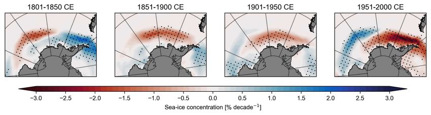
22                                                          Quentin Dalaiden et al.

734   3.1.4 Sea-ice cover

735   As for the atmospheric circulation, the sea-ice cover reconstructions rely totally
736   on the relationships between the assimilated variables and sea-ice cover as
737   represented by the model since this variable is not assimilated. Figure 2 shows
738   that the sea-ice concentration from our instrumental reconstruction is well
739   correlated with the observed sea-ice concentration from the National Snow and
740   Ice Data Center (NSIDC) over the 1979–2000 CE period. This is especially
741   true in the offshore regions where the interannual variability of the sea-ice
742   concentration is the highest. Indeed, the ocean along the West Antarctic coast
743   is nearly always covered by sea-ice (not shown). It is especially the case in the
744   Ross Sea sector and to a lesser extent in the Amundsen Sea sector. This means
745   that the interannual variability of the sea-ice concentration in this region is
746   weak. Consequently, the sea-ice concentration in that region cannot explain
747   the variability of the signal recorded in ice cores (e.g., snow accumulation and
748   δ 18 O). Therefore, given that the relationship between the ice core signal and
749   sea-ice concentration in that region is weak, the sea-ice concentration in that
750   region cannot be successfully reconstructed.
751        In order to quantify the sea-ice extent (i.e., oceanic surface covered by at
752   least 15% of ice) at the regional scale, we divide the West Antarctic sector
753   into two sectors following the geographical definitions of Parkinson (2019):
754   the Bellingshausen/Amundsen Sea sector (130◦ W-60◦ E) and Ross Sea sector
755   (160◦ E-130◦ W). It is important to stress that the overlapped period of 22
756   years between the NSIDC dataset and our reconstructions is short to evaluate
757   in detail our sea-ice extent reconstruction. Therefore, this limits our ability
758   to assess the quality of our reconstruction in terms of trends over the past
759   decades.
760        Our instrumental reconstruction displays a correlation coefficient r of 0.43
761   (p-value
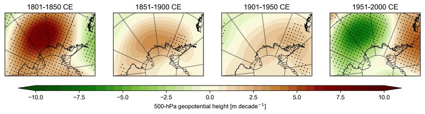
West Antarctic Climate reconstruction over the past two centuries                      23

779   sea-ice extent are in agreement with observations regarding the direction of
780   the change, our reconstructions underestimate the magnitude.

781   3.2 Reconstruction of the ASL and sea-ice in the West Antarctic sector over
782   the last 200 years

783   Now that we have evaluated the skill of our reconstructions during the recent
784   period, we can extend the reconstruction back in time. According to our an-
785   nual paleo-reconstruction of the ASL index (Fig. 5), the ASL displays three
786   main phases over the last two centuries. From 1800 CE to around 1840 CE, we
787   observe a positive linear trend (trend=0.34 std per decade; p-value0.05). From around 1940 CE,
790   the ASL displays a strong negative linear trend (trend=-0.30 std per decade;
791   p-value
You can also read