Gravity waves excited during a minor sudden stratospheric warming
←
→
Page content transcription
If your browser does not render page correctly, please read the page content below
Atmos. Chem. Phys., 18, 12915–12931, 2018
https://doi.org/10.5194/acp-18-12915-2018
© Author(s) 2018. This work is distributed under
the Creative Commons Attribution 4.0 License.

Gravity waves excited during a minor sudden
stratospheric warming
Andreas Dörnbrack1 , Sonja Gisinger1 , Natalie Kaifler1 , Tanja Christina Portele1 , Martina Bramberger1 ,
Markus Rapp1,2 , Michael Gerding3 , Jens Söder3 , Nedjeljka Žagar4 , and Damjan Jelić4
1 Institut
         für Physik der Atmosphäre, DLR Oberpfaffenhofen, Oberpfaffenhofen, Germany
2 Meteorologisches   Institut München, Ludwig-Maximilians-Universität München, Munich, Germany
3 Leibniz Institute of Atmospheric Physics at the University of Rostock, Kühlungsborn, Germany
4 University of Ljubljana, Faculty of Mathematics and Physics, Department of Physics, Ljubljana, Slovenia

Correspondence: Andreas Dörnbrack (andreas.doernbrack@dlr.de)

Received: 3 March 2018 – Discussion started: 13 March 2018
Revised: 23 July 2018 – Accepted: 2 August 2018 – Published: 7 September 2018

Abstract. An exceptionally deep upper-air sounding                tributed to spontaneous adjustment related to the polar-night
launched from Kiruna airport (67.82◦ N, 20.33◦ E) on 30 Jan-      jet (e.g., Sato, 2000; Sato, et al., 2012). The polar-night jet
uary 2016 stimulated the current investigation of internal        (PNJ) is a circumpolar stratospheric jet generated by the hi-
gravity waves excited during a minor sudden stratospheric         bernal cooling at high latitudes. The resulting meridional
warming (SSW) in the Arctic winter 2015/16. The analysis of       temperature gradient generates strong westerly winds. Due to
the radiosonde profile revealed large kinetic and potential en-   the underlying geostrophic or gradient wind balance, the PNJ
ergies in the upper stratosphere without any simultaneous en-     is predominantly a balanced phenomenon. However, in the
hancement of upper tropospheric and lower stratospheric val-      Northern Hemisphere the stratospheric polar vortex is usu-
ues. Upward-propagating inertia-gravity waves in the upper        ally disturbed by planetary waves, leading to different kinds
stratosphere and downward-propagating modes in the lower          of sudden stratospheric warmings (SSWs; e.g., Charlton and
stratosphere indicated a region of gravity wave generation        Polvani, 2007; Butler et al., 2015). Departures from the bal-
in the stratosphere. Two-dimensional wavelet analysis was         anced state lead to flow adjustment processes that can radi-
applied to vertical time series of temperature fluctuations in    ate as internal gravity waves from the jet stream (Limpasu-
order to determine the vertical propagation direction of the      van et al., 2011). This source mechanism to generate inter-
stratospheric gravity waves in 1-hourly high-resolution me-       nal gravity waves is known as spontaneous adjustment (e.g.,
teorological analyses and short-term forecasts. The separa-       Plougonven and Zhang, 2014).
tion of upward- and downward-propagating waves provided              Sato et al. (1999) and Sato (2000) was among the first
further evidence for a stratospheric source of gravity waves.     to suggest a similarity of the spontaneous adjustment at the
The scale-dependent decomposition of the flow into a bal-         tropospheric jet with that occurring in the stratosphere: her
anced component and inertia-gravity waves showed that co-         numerical simulations using a gravity-wave-resolving global
herent wave packets preferentially occurred at the inner edge     circulation model revealed a “dominance of downward prop-
of the Arctic polar vortex where a sub-vortex formed during       agation of wave energy around the polar-night jet in the
the minor SSW.                                                    winter hemisphere, suggesting the existence of gravity wave
                                                                  sources in the stratosphere.” More recently, Sato et al. (2012)
                                                                  used the gravity wave potential energy Ep as determined
                                                                  from their model simulations to document the longitudinal
1   Introduction                                                  and latitudinal distribution of gravity waves in the lower
                                                                  stratosphere in the southern winter hemisphere. They found
Stratospheric gravity waves observed at middle and high           significant downward energy fluxes associated with gravity
latitudes during wintertime conditions are occasionally at-

Published by Copernicus Publications on behalf of the European Geosciences Union.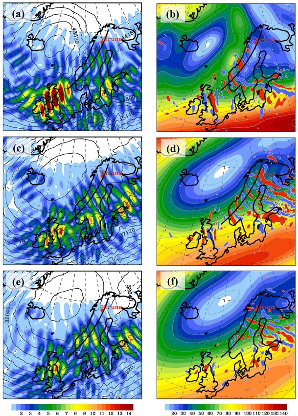
12916                                                   A. Dörnbrack et al.: Stratospheric excitation of inertia-gravity waves

waves in the lower stratosphere to the south of the Southern        non-orographic mechanisms such as spontaneous adjustment
Andes. Besides the downward spread of partially reflected           and jet instability around the edge of the stratospheric jet.”
mountain waves from the Andes, nonlinear processes in the           (p. 7813, Hindley et al., 2015).
stratosphere were mentioned as likely reasons.                         In situ observations in the stratosphere from 20 to 40 km of
   Direct observations of the excitation of stratospheric grav-     altitude are rare, especially at high latitudes. As in the stud-
ity waves by nonlinear processes are rare. Most of the ex-          ies by Yoshiki and Sato (2000) and Yoshiki et al. (2004),
isting studies concentrate on statistical aspects derived from      most of the published gravity wave analysis relies on oper-
high-vertical-resolution radiosondes (e.g., Yoshiki and Sato,       ational radiosondes launched once or twice a day. At high
2000; Yoshiki et al., 2004) or from ground-based (e.g.,             latitudes, only a few of these radiosondes reach altitudes
Whiteway et al., 1997; Whiteway and Duck, 1999; Khaykin             higher than 30 km in winter as the conventional 300–500 g
et al., 2015) and space-borne (e.g., Wu and Waters, 1996;           rubber balloons burst in the cold stratosphere. During the
Hindley et al., 2015) remote sensing observations. The ob-          METROSI1 campaign in northern Scandinavia, 3000 g rub-
servations of Whiteway at Eureka, Nunavut, Canada (80◦ N)           ber balloons were used by the LITOS group (Theuerkauf et
during four Arctic winters showed an increase in strato-            al., 2011; Haack et al., 2014; Schneider et al., 2017) study-
spheric gravity wave energy in the vicinity of the PNJ. More        ing fine-scale turbulence in the upper troposphere–lower
precisely, the amount of upper stratospheric wave energy was        stratosphere (UTLS) mainly from Andøya, Norway (69◦ N,
maximum within the PNJ at the edge of the polar vortex,             15.7◦ E). A common deployment phase of their turbulence
minimum near the vortex center, and intermediate outside the        sensor took place in Kiruna, Sweden (68◦ N, 20◦ E) dur-
vortex (Whiteway et al., 1997).                                     ing GW-LCYCLE 22 . Operational forecasts of the integrated
   Yoshiki and Sato (2000) analyzed radiosonde observations         forecast system (IFS) of the European Centre for Medium-
from 33 polar stations over a period of 10 years to investi-        Range Weather Forecasts (ECMWF) predicted the appear-
gate gravity waves in the lower stratosphere, inter alia, by        ance of wave-like structures in the stratosphere northwest of
examining the correlation between the gravity wave intensity        Kiruna. The close proximity of the predicted waves and the
(expressed as kinetic energy EK ) in the lower stratosphere         relatively weak stratospheric winds (50 m s−1 ) led to the de-
and the mean wind. For the Arctic, they found a high corre-         cision to launch a radiosonde with one of the large 3000 g
lation of EK with the surface wind, whereas EK correlates           balloons on the morning of 30 January 2016.
with the stratospheric wind in the Antarctic. The dominance            The relatively weak stratospheric winds over northern
of upward-propagating gravity waves points to orographic            Scandinavia were associated with the southward displace-
sources in the Arctic, whereas the high percentage of down-         ment of the Arctic polar vortex during a minor SSW
ward energy propagation in the lower stratosphere found for         (Matthias et al., 2016; Manney and Lawrence, 2016). The
winter and spring suggests other gravity wave sources in            stratosphere in the northern hemispheric winter 2015/2016
the Antarctic. Yoshiki and Sato (2000) speculated that one          was exceptionally cold as the polar vortex was essentially
source candidate is likely to be the PNJ. Yoshiki et al. (2004)     barotropic and centered near the North Pole in early win-
investigated the temporal variation of the gravity wave en-         ter months (Matthias et al., 2016). These conditions are usu-
ergy in the lower stratosphere with respect to the position         ally associated with weak planetary wave activity. Indeed,
of the polar vortex by using the equivalent latitude coordi-        Matthias et al. (2016) showed that the planetary wavenum-
nate for the Antarctic station Syowa (69◦ S, 40◦ E). In agree-      ber 1 amplitude was exceptionally small in November–
ment with the results of Whiteway et al. (1997), gravity wave       December 2015 compared to 37 years of ERA-Interim and
energy is enhanced when the edge of the polar vortex ap-            68 years of NCAR/NCEP reanalysis data. Planetary waves of
proaches Syowa Station. Surprisingly, they found an espe-           zonal wavenumber 1 were amplified during the second half
cially large enhancement during the breakdown phase of the          of January 2016 and three consecutive minor SSWs occurred
polar vortex in spring. As they write in their paper: “As it        before the final breakdown of the polar vortex at the begin-
is difficult to explain the energy enhancements only by the         ning of March 2016 (Manney and Lawrence, 2016).
variation in horizontal wind and/or the static stability, the en-      This paper presents a case study analyzing a series of ra-
hancements of wave activity at the edge of the polar vortex         diosonde observations during the first minor SSW at the end
are likely to contribute to the energy enhancements by wave         of January 2016. We focus on the analysis of the 3000 g bal-
generation in the stratosphere.”.                                   loon ascent of 30 January 2016, which reached an excep-
   Hindley et al. (2015) suggested that the distributions of        tional altitude of 38.1 km. The paper documents this event by
increased stratospheric Ep values in the Southern Hemi-
sphere eastwards of around 20◦ E, as determined from                   1 METROSI: Mesoscale Processes in Troposphere–Stratosphere
global positioning system radio occultation (GPS-RO) data           Interaction.
from the COSMIC satellite constellation, might be due to               2 The GW-LCYCLE 2 campaign was a coordinated effort of
stratospheric sources. Their nearly homogeneous distribu-           multiple German institutions to combine ground-based, balloon-
tion of enhanced Ep values especially indicates “... a zon-         borne, airborne, and satellite instruments to investigate the life cycle
ally uniform distribution of small amplitude waves from             of gravity waves above Scandinavia in January and February 2016.

Atmos. Chem. Phys., 18, 12915–12931, 2018                                             www.atmos-chem-phys.net/18/12915/2018/
A. Dörnbrack et al.: Stratospheric excitation of inertia-gravity waves                                                         12917

combining and comparing the measurements with numerical               2.2   Meteorological data from the IFS
weather prediction (NWP) analyses and forecasts. The char-
acteristics and the sources of the observed stratospheric grav-       Operational analyses and high-resolution (HRES) forecasts
ity waves are investigated. We show that the characteristics          of the ECMWF’s IFS are used to provide meteorologi-
of the stratospheric gravity waves determined from observa-           cal data characterizing the ambient atmospheric conditions
tions and model data suggest a stratospheric source. Section 2        and the resolved stratospheric gravity waves. The IFS is a
contains information about the data sources and the methods           global, hydrostatic NWP model with semi-implicit time step-
to analyze them. Section 3 reviews the particular meteorolog-         ping (Robert et al., 1972) and semi-Lagrangian advection
ical situation and portrays the transition of the stratospheric       (Ritchie, 1988). Two different IFS cycles are available for
flow regime over northern Scandinavia. Section 4 presents             January 2016. The operational IFS cycle 41r1 provides fields
the vertical profiles of the deep radiosonde sounding and             with a horizontal resolution of about 16 km (TL 1279) and
continues with an analysis of the observed gravity waves.             137 vertical model levels (L137). The IFS cycle 41r2 has a
Section 5 investigates the wave properties derived from the           horizontal resolution of about 9 km (TCo 1279) and the same
IFS data starting with a comparison to the observations, and          number of vertical levels3 (Hólm et al., 2016). With the cu-
Sect. 6 concludes the paper.                                          bic spectral truncation used for cycle 41r2 the shortest re-
                                                                      solved wave is represented by four rather than two grid points
                                                                      and the octahedral grid is globally more uniform than the
2     Data sources and analysis methods                               previously used reduced Gaussian grid (Malardel and Wedi,
                                                                      2016). The model top of both IFS cycles is 0.01 hPa. The
2.1    Radiosonde soundings                                           IFS cycle 41r2 was in its pre-operational mode and prod-
                                                                      ucts were disseminated among the users. Ehard et al. (2018)
Nine consecutive radiosondes were launched from Kiruna
                                                                      showed that both IFS cycles reproduce the temporal evolu-
airport (67.82◦ N, 20.33◦ E) on 29 and 30 January 2016.
                                                                      tion of the observed gravity wave potential energy density
The radiosondes were the Vaisala model RS41-SG (Vaisala,
                                                                      EP in the middle stratosphere above Sodankylä, Finland cor-
2017). The measured horizontal wind components u and v
                                                                      rectly for the months December 2015 to March 2016. There-
and temperature T have a temporal resolution of 1 s. As-
                                                                      fore, the IFS cycle 41r2 was selected for the present analysis
suming a mean balloon ascent rate of 5 m s−1 the atmo-
                                                                      and profiles of the IFS cycle 41r1 are only shown for com-
spheric variables u, v, and T have a vertical resolution of
                                                                      parison in Fig. 3.
about 5 m. For the wave analysis the radiosonde data were
interpolated onto an equidistant vertical grid with 25 m res-         2.3   Scale-dependent modal decomposition
olution. The gravity wave properties of all nine soundings
were analyzed, whereby the wave perturbations u0 , v 0 , and          The IFS cycle 41r2 analyses of 30 January 2016 00:00,
T 0 were calculated as differences between the actual quan-           06:00, and 12:00 UTC are decomposed into inertia-gravity
tities and the respective background profiles hui, hvi, and           waves (IGWs) and Rossby waves using the 3-D normal-
hT i. The background profiles were determined by a second-            mode function decomposition as described by Žagar et
order polynomial fit of u, v, and T in the troposphere and            al. (2015). The modal decomposition projects the 3-D wind
in the stratosphere, respectively. Additionally, a 5 km run-          and geopotential height fields onto a set of predefined ba-
ning mean was removed from the perturbation profiles and              sis functions for a realistic model stratification. The basis
added to the background (Lane et al., 2000, 2003). The lat-           functions are derived from an eigenvalue problem (Kasahara,
ter step reduces the arbitrariness of the polynomial fit de-          1976, 1978; Kasahara and Puri, 1981). The eigenfunctions
pending on the particular shape of the measured profiles              are solutions to two dispersion relationships that correspond
and avoids outliers in the perturbation profiles. The specific        to the vorticity-dominated Rossby waves and divergence-
kinetic and  potential
                       energies are    calculated according to       dominated IGWs on the sphere (Kasahara, 1976). A dis-
          1  0 2  0 2              g2 T 0 2
EK = 2 u + v and EP = 2N2                   2 , respectively, where   tinct advantage of the applied decomposition is the 3-D or-

the overbar denotes averages taken over selected layers in            thogonality of the basis functions, which enables the fil-
the troposphere or stratosphere. Stokes parameters and rotary         tering of any mode of oscillations in physical space. Ža-
spectra are used to describe essential parameters of the grav-        gar et al. (2017) applied the modal decomposition to recent
ity waves                                                             ECMWF analyses and discussed the IGW features across
          retrieved from the perturbation wind components
 u0 , v 0 and from T 0 . The associated techniques are well doc-      the resolved spectrum. Their examples of propagating linear
umented and described, e.g., by Vincent (1984), Eckermann             IGWs in the data analyzed at selected time steps showed that
and Vincent (1989), Eckermann (1996), Vincent et al. (1997),             3 The    IFS   cycle    41r2    became      operational   on
and Murphy et al. (2014).
                                                                      8      March    2016;    see    https://software.ecmwf.int/wiki/
                                                                      display/FCST/Implementation+of+IFS+cycle+41r2               and
                                                                      http://www.ecmwf.int/en/about/media-centre/news/2016/
                                                                      new-forecast-model-cycle-brings-highest-ever-resolution.

www.atmos-chem-phys.net/18/12915/2018/                                              Atmos. Chem. Phys., 18, 12915–12931, 2018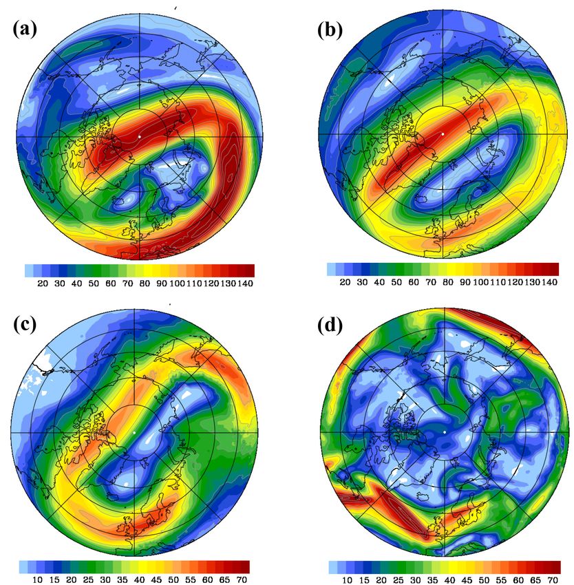
12918                                                  A. Dörnbrack et al.: Stratospheric excitation of inertia-gravity waves

the modal decomposition is a useful complementary tool for
studying internal gravity waves.
   The results of Žagar et al. (2017) suggest that current
ECMWF analyses resolve IGWs in synoptic scales and in
large mesoscale features with scales larger than 500 km well.
For smaller scales, such as studied here, the model spectrum
of IGWs deviates from the expected −5/3 slope, suggestive
of a lack of variability. Our comparison of the model with ob-
servations will illustrate some aspects of the missing variabil-
ity. By filtering out zonal wavenumbers smaller than 30, we
focus on inertia-gravity waves with horizontal wavelengths
shorter than 660 km (at 60◦ N). The IGWs are evolving on the
background flow that is represented by the Rossby waves and
this flow component is denoted by BAL (balanced). The bal-
anced component is presented without scale-dependent filter-
ing.

2.4   Two-dimensional wavelet analysis

In addition to the normal-mode decomposition, we ana-
lyze IFS cycle 41r2 temperatures in the time frame between
26 January and 1 February 2016 for gravity waves. For this         Figure 1. Magnitude of the balanced wind VHBAL (m s−1 , color
purpose, the 1-hourly temperature fields of the IFS cycle 41r2     shaded) from the normal-mode analysis at pressure surfaces of
above Kiruna are interpolated on an equidistant grid with          1 hPa (a), 5 hPa (b), 50 hPa (c), and 250 hPa (d) valid on 30 Jan-
500 m vertical resolution in the altitude range of 12 to 65 km.    uary 2016 06:00 UTC.
This dataset might be considered as “virtual” ground-based
measurements, e.g., by a Rayleigh lidar, emulating a com-
mon type of observations during Arctic field campaigns (e.g.,      tigate the evolution of the gravity wave field around 30 Jan-
Baumgarten et al., 2015; Hildebrand et al., 2017; Kaifler et       uary relative spectrograms are determined. While Kaifler et
al., 2015). Temperature perturbations T 0 assigned to gravity      al. (2017) applied a seasonal average for comparison, here,
waves are determined from the local temperatures relative          we use the global spectrogram computed over the whole
to an area mean between 65◦ N, 10◦ E and 70◦ N, 30◦ E. In          period from 26 January until 1 February 2016 as a refer-
this way, perturbations with scales larger than 600–900 km         ence. Effectively, the relative spectrogram is the difference
horizontal wavelength are effectively removed. No vertical         between the spectrogram computed for selected intervals and
or temporal filters were applied. We cross-checked with the        this global spectrogram. As the latter contains the sum of all
methods commonly applied to Rayleigh lidar measurements            contributions from waves, the values of the relative spectro-
(Ehard et al., 2015) and found that (i) the problems arising       grams are negative. The highest value zero means that the
in vertical filtering due to the tropospheric T gradient and       wave packet in question was detected in the selected interval
the tropopause were circumvented, (ii) mountain wave signa-        only.
tures are sustained compared to temporal filtering methods,
and (iii) our results on transient gravity waves in the strato-    3     Meteorological situation
sphere were unaffected. In order to distinguish upward- and
downward-propagating gravity waves, we applied directional         3.1    Circulation pattern
two-dimensional Morlet wavelets (Wang and Lu, 2010) to
T 0 as a function of altitude and time. The wavelet analysis       Weak stratospheric planetary wave activity caused excep-
allows for separation of gravity waves of different vertical       tionally low temperatures inside the Arctic polar vortex in
wavelengths and phase speeds while preserving temporal and         the early winter months 2015/2016 (Matthias et al., 2016;
vertical information. Using this method, the occurrence and        Dörnbrack et al., 2017a). The polar vortex remained cold
activity of quasi-stationary as well as transient upward- and      until the beginning of March 2016 (Manney and Lawrence,
downward-propagating waves is investigated and the vertical        2016). Starting in mid-January 2016, the polar vortex became
wavelength λz and ground-based vertical phase speed cPz of         disturbed by planetary waves and three minor SSWs that oc-
dominant gravity waves are estimated. Recently, this tech-         curred at the end of January and mid-February 2016. During
nique was developed and applied successfully to time series        the January 2016 minor SSW, the center of the polar vortex
of ground-based Rayleigh lidar profiles. It is described and       was displaced from the pole region and shifted southward
discussed in detail by Kaifler et al. (2015, 2017). To inves-      between northern Scandinavia and Svalbard. The circumpo-

Atmos. Chem. Phys., 18, 12915–12931, 2018                                          www.atmos-chem-phys.net/18/12915/2018/
A. Dörnbrack et al.: Stratospheric excitation of inertia-gravity waves                                                           12919

lar PNJ elongated in the west–east direction above Eurasia,
leading to regions of strong curvature at the vertices over the
northern Atlantic and over Siberia. Figure 1a, b, and c illus-
trate the twist of the vortex and its distortion by means of the
magnitude of the balanced wind VHBAL at three stratospheric
pressure levels valid at 06:00 UTC on 30 January 2016.
   Near the stratopause at 1 hPa, the PNJ was strongly de-
celerated to values VHBAL < 30 m s−1 in the region south
of Greenland (Fig. 1a). Above Europe, the jet core was lo-
cated south of the Alps and attained maximum winds of
more than 120 m s−1 at this pressure level. Northern Scan-
dinavia was located in the center of the polar vortex where
VHBAL < 20 m s−1 . However, north of Scotland and west of
Scandinavia, a jet branch separated from the inner edge of the
PNJ in the strong curvature region over the northern Atlantic
and a weak rotary circulation formed inside the polar vortex
(Fig. 1a). A band of enhanced balanced winds VHBAL ≈ 40–
50 m s−1 is also visible at the same location at 5 hPa (Fig. 1b)
extending towards northern Scandinavia. Otherwise, Fig. 1b
documents a closed circulation of the polar vortex with VHBAL
> 80 m s−1 in the elongated parts and weaker winds near
the eastern and western vertices. The separated upper strato-
spheric branch of the PNJ was on top of a region of VHBAL
≈ 30–50 m s−1 in the middle stratosphere at 50 hPa (Fig. 1c).      Figure 2. Altitude–time sections of the horizontal wind VH in
The nearly unidirectional strong southwesterly stratospheric       m s−1 (a) and the absolute temperature in K (b) as a composite of
winds over southern and northern Scandinavia suggest favor-        1-hourly short-term HRES forecasts and 6-hourly operational anal-
able propagation conditions for gravity waves.                     yses from the IFS cycle 41r2 above Kiruna, Sweden. The thin black
   Near the tropopause level at 250 hPa, three jet streaks with    lines are the logarithm of the potential temperature with constant in-
maximum VHBAL ≈ 70 m s−1 stretched across the North At-            crements of 0.05. The vertical black lines mark the radiosonde paths
                                                                   of the nine soundings mentioned in the text.
lantic and the North Sea (Fig. 1d). They led to high tro-
pospheric winds over Scotland and southern Scandinavia.
Northern Scandinavia was north of the baroclinic zone as-
sociated with the polar front and influenced by a weak             4     The deep radiosonde sounding of 30 January 2016
tropopause jet with maximum VHBAL ≈ 25 m s−1 oriented
nearly perpendicular to the mountain range.                        4.1    Radiosounding

                                                                   On 29 and 30 January 2016, altogether nine radiosondes
3.2   Temporal evolution above Kiruna
                                                                   were launched from Kiruna airport. Only two radiosondes
                                                                   ascended to altitudes higher than 30 km. For these upper-air
Figure 2 illustrates the temporal evolution of the horizontal      soundings 3000 g rubber balloons (TOTEX, TX3000) were
wind VH (Fig. 2a) and the absolute temperature T (Fig. 2b)         employed; the smaller 500 or 600 g balloons used for the
over Kiruna in the period from 26 January until 1 Febru-           other soundings burst in the cold layer of the polar vortex (see
ary 2016. In general, this period is characterized by a regime     vertical trajectories in Fig. 2b). The minimum temperature
transition of the stratospheric flow during the minor warm-        measured during these two days was TMIN ≈ 180 K (−93 ◦ C)
ing. The gradual decline of the horizontal wind (Fig. 2a)          on 29 January at 08:45 UTC at 25 km of altitude (not shown).
and the descent of the cold layer (Fig. 2b) in the strato-         However, the observed TMIN increased by about 10 K above
sphere reflect the southward displacement of the polar vor-        Kiruna during 24 h due to the adiabatic descent associated
tex and the approach of its center. After 30 January 2016,         with the southward shift of the polar vortex. Nevertheless,
the conditions over Kiruna are marked by light horizontal          only the large 3000 g balloons could penetrate the cold strato-
wind VH < 20 m s−1 , a warmer stratopause of up to 290 K,          spheric layer without bursting.
and an about 3–4 km lower cold stratospheric layer. In this           On 30 January 2016, the 3000 g rubber balloon was
layer, the IFS temperature was about 4 to 8 K warmer than          released at 09:08:45 UTC and the ascent lasted until
at the beginning of the period. During the regime transition,      10:52:17 UTC, reaching an altitude of 38.1 km. During this
VH , T , and 2 display wave-like perturbations in the strato-      time, the balloon drifted about 160 km to the northeast. Fig-
sphere (Fig. 2).                                                   ure 3a shows the temperature profile as a function of alti-

www.atmos-chem-phys.net/18/12915/2018/                                             Atmos. Chem. Phys., 18, 12915–12931, 2018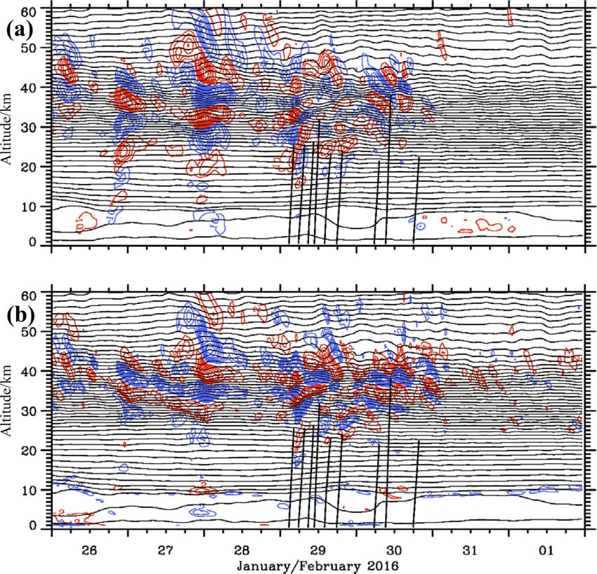
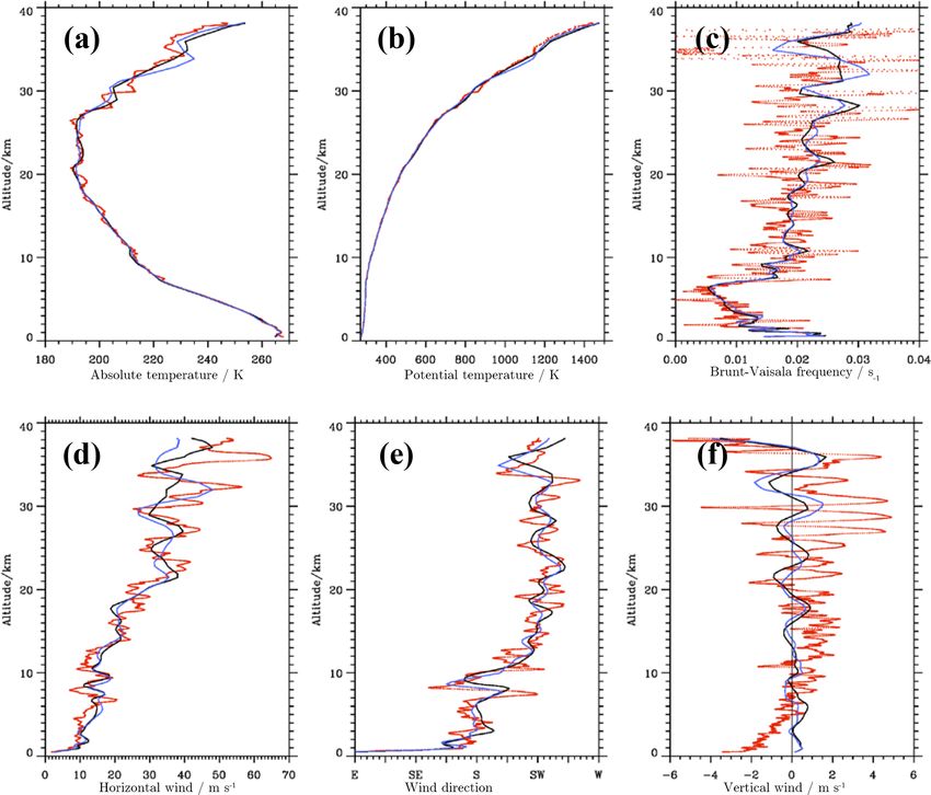
12920                                                     A. Dörnbrack et al.: Stratospheric excitation of inertia-gravity waves

Figure 3. Vertical profiles of the absolute temperature (a), potential temperature (b), buoyancy frequency (c), horizontal wind (d), wind
direction (e), and vertical wind (f). Red dots: radiosonde observations from the 30 January 2016 09:08 UTC ascent. Solid lines: ECMWF IFS
operational HRES forecasts interpolated in space and time on the balloon trajectory from cycle 41r1 (black) and 41r2 (blue). The ECMWF
vertical winds are multiplied by a factor of 10. The vertical winds from the balloon sounding are calculated as the difference of the local
ascent rate and a mean ascent rate of 6.1 m s−1 determined as an integral value over the whole profile.

tude. The bow-shaped profile is characterized by a minimum              at 1 km to about 50 m s−1 at 38 km of altitude. From 29
temperature of about 190 K (−83 ◦ C) inside the polar vor-              to 30 January 2016, the mean horizontal wind in the lower
tex between 20 and 28 km of altitude. This value is about               troposphere decreased from 20 m s−1 (not shown) to about
45 K lower than the temperature at the tropopause, which is             10 m s−1 (Fig. 3d). The main features of the VH profile are
marked by the strong increase in static stability at ≈ 8 km of          fluctuations with an apparent vertical wavelength of about λz
altitude (Fig. 3c). Above 28 km of altitude the temperature in-         ≈ 3–5 km and shorter oscillations with λz ≈ 1 km. The am-
creased by about 55 K and attained similar values at 38.1 km            plitude of the longer waves increases with height, whereas
as measured in the troposphere at around 6 km of altitude.              the shorter waves almost vanish above 28 km of altitude. Fig-
The other characteristic of the temperature profile is the ex-          ure 3e shows the turning of the wind from southerlies in the
istence of wave-like oscillations. They are pronounced be-              troposphere to southwesterlies, which dominated the strato-
tween 10 and 20 km and above about 28 km of altitude. The               spheric flow above northern Scandinavia on 30 January 2016.
amplitude of the fluctuations increases with altitude, which            The wave-like oscillations of the wind direction reflect the
is also visible in the profile of the potential temperature 2           same kind of pattern as found in the VH profile. The verti-
(Fig. 3b). The buoyancy frequency as calculated from the 2              cal wind as derived from the balloon ascent rates and from
profile shows substantial oscillations with increasing ampli-           the IFS show a growth in amplitude with increasing altitude
tudes in the stratosphere (Fig. 3c). In the upper range of the          (Fig. 3f). However, the amplitudes and vertical wavelengths
profile, very small and even negative values were calculated,           differ due to the absence of high-frequency waves in the IFS.
indicating the existence of vertically separated mixing layers.         In the following subsection, the properties of the observed
   Overall, the magnitude of the horizontal wind VH as de-              gravity waves are analyzed.
picted in Fig. 3d increases nearly linearly from about 5 m s−1

Atmos. Chem. Phys., 18, 12915–12931, 2018                                                www.atmos-chem-phys.net/18/12915/2018/
A. Dörnbrack et al.: Stratospheric excitation of inertia-gravity waves                                                                      12921

Table 1. Kinetic and potential energy densities EK (m2 s−2 ) and            Table 2. As for Table 1 for the 29 January 2016 10:42 UTC sound-
EP (J kg−1 ) for the 30 January 2016 09:08 UTC radiosonde sound-            ing and IFS temperature perturbation on 29 January 2016.
ings (RSs). Additionally, the ratio R RS of the power of the upward-
propagating part of the rotary spectrum to the total power is given.                                       29 January 2016
Mean gravity wave potential energy densities in J kg−1 derived                                 RS                            IFS
from vertical time series of the IFS temperature perturbations as                                                   up
                                                                                         EP   EK    R RS   EPmw   EP     EPdown     R IFS   EPtot
shown in Fig. 7b. EP values are classified for quasi-stationary
mountain waves (EPmw , |cPz | ≤ 0.036 m s−1 ), upward-propagating             1–8 km      5    16   0.74
           up                                                                 12–20 km    3    12   0.47      0     0           2   0.21       2
waves (EP , cPz < 0.036 m s−1 ), downward-propagating waves                   20–28 km    5    21   0.43      0     1           5   0.17       7
(EPdown , cPz > 0.036 m s−1 ), and the total value EPtot from the 2-          30–38 km                        1     8          25   0.24      39
D wavelet analysis. Due to the nonlinear average of T 0 in the cal-           40–48 km                        0    15           6   0.72      21
culation of the gravity wave potential energy densities, the sum
           up
EPmw + EP + EPdown deviates slightly from EPtot . For the IFS anal-
                                       up           up
ysis R IFS is calculated as the ratio EP /(EPmw + EP + EPdown ).
                                                                            stratospheric layers on 30 January. This means that the ob-
                                                                            served waves are dominated by intrinsic frequencies much
                                30 January 2016
                                                                            smaller than the buoyancy frequency N ∼     = 0.02 s−1 (Fig. 3c);
                   RS                             IFS                       i.e., this analysis points to essentially low-frequency, hydro-
                                         up
             EP    EK   R RS    EPmw   EP     EPdown        R IFS   EPtot   static inertia-gravity waves (Fritts and Alexander, 2003).
  1–8 km      10    8    0.78                                                  Stokes analysis was applied to determine essential grav-
  12–20 km     5   10    0.51      0     1              0   0.60       1    ity wave parameters (e. g., Eckermann and Vincent, 1989;
  20–28 km     9   23    0.62      0     2              0   0.68       3    Vincent et al., 1997). First, the degree of polarization was
  30–38 km    25   79    0.76      3    14              5   0.66      29
  40–48 km                         0     6              3   0.65      11    determined to be 0.8 between 30 and 38 km of altitude for
                                                                            the 30 January 2016 09:08 UTC profile. This value becomes
                                                                            gradually smaller for the lower stratospheric layers (0.7 for
                                                                            20–28 km and 0.3 for 12–20 km). Values close to 1 point
4.2   Gravity wave analysis                                                 to monochromatic waves, while values close to zero indi-
                                                                            cate a random wave field (Vincent et al., 1997). The middle
As listed in Table 1, the vertically averaged kinetic and                   stratospheric fluctuations determined from the radiosonde
potential energies EK and EP in the troposphere (1–8 km)                    profile are thus dominated by coherent gravity waves obey-
and lower stratosphere (12–20 km) of the deep sounding                      ing the linear dispersion relation. The ratio /f determines
on 30 January 2016 have values of EK = 8 (10) J kg−1 and                    the hodographs of u0 and v 0 and can be calculated by Stokes
EP = 10 (5) J kg−1 , respectively. These values are close to                analysis. The small values of /f ≈ 2.1 for 30–38 km and
the mean over all nine soundings of EK = 10 (9) J kg−1                      /f ≈ 3.2 for 20–28 km support the former finding that the
and EP = 7 (4) J kg−1 for the troposphere and lower strato-                 observed waves are most likely low-frequency inertia-gravity
sphere. In the middle stratosphere (20–28 km), vertically av-               waves. On the other hand, the larger ratio of /f ≈ 12 de-
eraged energies EK and EP increase to values of 23 and                      rived for the lower stratosphere might point to an influence of
9 J kg−1 , respectively. Compared to the earlier deep sound-                different types of gravity waves; see the discussion in Sect. 6.
ing on 29 January 2016 10:42 UTC (reaching only 31 km                          The vertical wavelength determined from the power spec-
of peak altitude), there is nearly a doubling of tropospheric               tra of u0 and v 0 is λz ≈ 4 km in all altitude layers. The hori-
and stratospheric gravity wave potential energies, whereas                  zontal wavelength determined by using /f from the Stokes
the tropospheric kinetic energy is halved (cf. Table 2 with                 analysis increases with height from λH ≈ 50 km for 12–
Table 1). The reduction of tropospheric gravity wave ki-                    20 km of altitude, to λH ≈ 220 km (20–28 km), and to λH ≈
netic energy goes along with weakening tropospheric winds                   330 km between 30 and 38 km. Applying the Stokes analy-
as mentioned above. High energy values are obtained in                      sis, the horizontal propagation direction turns anticlockwise
the upper stratosphere (30–38 km) of EK = 79 J kg−1 and                     from west–northwest in the lower stratosphere, to west be-
EP = 25 J kg−1 on 30 January (Table 1). Besides the increase                tween 20 and 28 km, and to west–southwest in the upper-
in EK and EP in the stratosphere above 20 km of altitude,                   most layer (30–38 km). Therefore, the inertia-gravity waves
we found a dominance of the kinetic energy in these lay-                    with an estimated intrinsic phase speed cp between 13 and
ers for both deep soundings of 29 and 30 January 2016 (Ta-                  15 m s−1 propagated against the ambient stratospheric flow.
bles 1, 2). According to Sato and Yoshiki (2008), EK val-                   As the magnitude of the intrinsic phase speed cp is smaller
ues larger than EP point to inertia-gravity waves with an                   than the ambient wind VH , the gravity waves propagate
intrinsic frequency  close to the inertia frequency f as                 northeastward with respect to the ground.
Ep /EK = 2 − f 2 / 2 + f 2 based on linear theory; see                       Both the rotary spectra and the Stokes analysis can be used
Gill (1982). Applying this relationship results in an estimate              to estimate the dominant vertical propagation direction for
of the scaled intrinsic frequency being /f ≈ 1.4–1.7 for the               the deep soundings. For this purpose, the ratio R RS of the

www.atmos-chem-phys.net/18/12915/2018/                                                    Atmos. Chem. Phys., 18, 12915–12931, 2018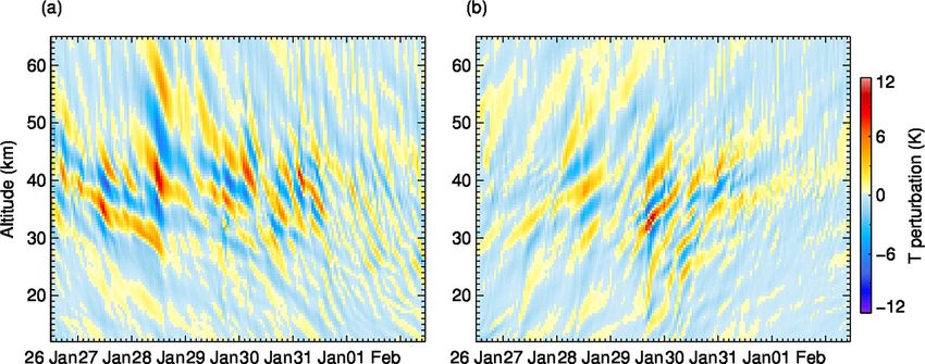
12922 A. Dörnbrack et al.: Stratospheric excitation of inertia-gravity waves
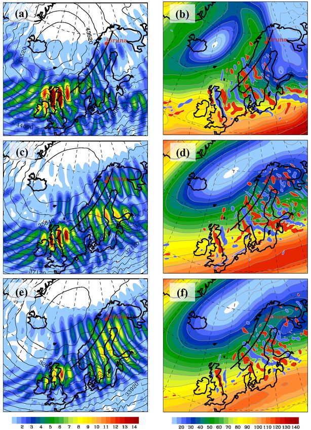
Figure 4. (a, c, d) Composite of the magnitude of VHIGW (m s−1 , Figure 5. Same as Fig. 4 for 12:00 UTC on 30 January 2016.
color shaded) from the normal-mode analysis and the geopoten-
tial height (m, black contour lines) from IFS operational analyses.
(b, d, f) Composite of the magnitude of the balanced wind VHBAL
indicates downward-propagating waves in an extended alti-
(m s−1 , color shaded) from the normal-mode analysis and the hori- tude range between 12 and 28 km (Table 2). Assuming the
zontal divergence (values larger or smaller than ±2 × 10⁻⁴ s−1 are
downward-propagating waves are radiated from the same el-
filled with red and blue, respectively) from operational analyses.
The plots are at 1 hPa (∼ 48 km; a, b), 3 hPa (∼40 km; c, d), and
evated source, the excitation likely occurred shortly before
5 hPa (∼ 36 km; e, f) and they are valid at 06:00 UTC on 30 Jan- 29 January 2016 ∼ 11:00 UTC at an altitude above 28 km
uary 2016. The black line marks the baseline of the vertical sections and its effects are still detected in the lower stratosphere 22 h
shown in Fig. 6. later.
5 Gravity wave analysis of IFS data
power of the upward-propagating part of the rotary spec-
trum, i.e., the positive part of the Fourier spectrum of u0 +iv 0 5.1 Comparison of radiosonde observations with IFS
(Vincent, 1984), to the total power is calculated and listed
in Tables 1 and 2. For R RS > 0.6 upward wave propagation Vertical profiles of different variables from the ECMWF IFS
can be assumed because there is a significant bias towards interpolated on the balloon trajectory in space and time are
upward propagation of inertia-gravity waves (Guest et al., shown in Fig. 3. The IFS data used for this comparison are
2000). R RS is 0.78, 0.51, 0.62, and 0.76 for the layers 1–8, the short-term HRES forecasts of the IFS cycles 41r1 and
12–20, 20–28, and 30–38 km of altitude, respectively, for the 41r2 at lead times +9, +10, and +11 h of the 00:00 UTC
30 January 2016 09:08 UTC sounding. Thus, except in the forecast run of 30 January 2016.
layer from 12 to 20 km of altitude, the dominant propagation The observed and simulated temperature profiles agree
direction is upward. This result is supported by the Stokes qualitatively and quantitatively very well up to an altitude of
analysis, which gives downward propagation exclusively in 28 km. Obviously, the IFS profiles cannot reproduce the fine-
the same layer from 12 to 20 km of altitude. The deep ra- scale oscillations found in the temperature sounding. How-
diosonde sounding from 29 January 2016 10:42 UTC clearly ever, the general temperature decrease and the cold strato-
Atmos. Chem. Phys., 18, 12915–12931, 2018 www.atmos-chem-phys.net/18/12915/2018/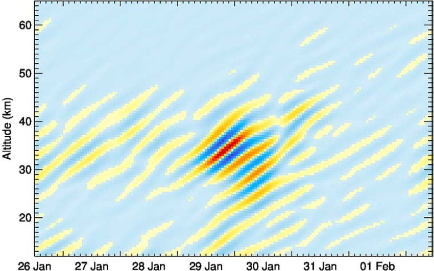
A. Dörnbrack et al.: Stratospheric excitation of inertia-gravity waves                                                        12923

spheric layer are quantitatively well captured by the model.
Higher up, the profile of IFS cycle 41r2 captures the lo-
cal T maximum at about 34 km well, whereas the coarser-
resolved cycle 41r1 underestimates the stratospheric fluctu-
ations. Comparing the two different IFS cycles, it becomes
clear that the IFS cycle 41r1 has a smaller wave amplitude
1T ≈ 1.4 K, whereas the IFS cycle 41r2 has a nearly realis-
tic 1T ≈ 5 K. Deviations between the IFS and the observa-
tion by up to 5 K exist in the upper part of the sounding.
   Examining the VH profiles, the IFS cycles simulate os-
cillations with a vertical wavelength of λz ≈ 5–6 km, which
are longer than the observed ones. Moreover, the amplitude
of the resolved gravity waves is underestimated by the IFS.
Nevertheless, the numerical results of the IFS suggest that
the resolved gravity wave activity contains a fair degree of
realism in the upper stratosphere, confirming the findings of
Dörnbrack et al. (2017a). Moreover, both the overall verti-
cal change in wind and wind direction are well captured, es-
pecially by the IFS cycle 41r2. It should be noted that all
the radiosonde profiles were not assimilated into the IFS and
therefore constitute independent measurements.

5.2   Inertia-gravity waves

Figures 4 to 6 depict composites of operational analyses and
the scale-dependent modal decomposition of the IFS cycle
41r2 at selected times on 30 January 2016. Figures 4 and 5
juxtapose the magnitude of the IGW component of the hor-
izontal wind VHIGW (left column) and the horizontal diver-
gence (DIV) patterns from the analyses (right column) at the
upper stratospheric pressure surfaces of 1, 3, and 5 hPa for
06:00 and 12:00 UTC, respectively. The background fields in      Figure 6. Composite of the magnitude of the balanced wind VHBAL
the individual panels of Figs. 4 and 5 are the geopotential      (m s−1 , color shaded) and the unbalanced zonal wind U IGW (ar-
height Z and the magnitude of the balanced wind VHBAL , re-      eas with negative values larger than −3 m s−1 and positive values
spectively. Note that both Z and DIV are extracted directly      smaller than 3 m s−1 are filled with blue and red, respectively) from
from the ECMWF data archive. Thus, the particular patterns       the normal-mode analysis. The vertical sections are along the base-
of divergence and IGWs as computed by the modal decom-           line sketched in Figs. 4 and 5 and they are valid on 30 January 2016
position can be considered as independent diagnostics of the     at 00:00 UTC (a), 06:00 UTC (b), and 12:00 UTC (c).
unbalanced flow in the IFS.
   Consecutive VHIGW maxima mark groups of inertia-gravity
waves of different orientations and intensities. There are two
groups over and in the lee of Scotland and southern Scandi-      much weaker, i.e., it reveals smaller VHIGW amplitudes, com-
navia and another one over northern Scandinavia, best seen       pared to the others and, importantly, shows a transient be-
in Fig. 4c. All groups reside along the inner edge of the po-    havior between 06:00 and 12:00 UTC. In the following, we
lar vortex (Figs. 4a, c, e and 5a, c, e). The two groups over    concentrate on this wave group over northern Scandinavia.
and in the lee of Scotland and southern Scandinavia were            Two distinct features are relevant for the interpretation of
likely excited by topographic forcing. This hypothesis is sup-   the radiosonde observations. First, the inertia-gravity waves
ported by the stationarity of the wave groups at different       are located in a region where the stratospheric jet is deceler-
times; e.g., compare Figs. 4e and 5e. The VHIGW maxima are       ated as visible by the declining wind VHBAL towards the north-
correlated with undulations in the geopotential height Z at      east. There, the formation of the little vortex seen in VHBAL
the different pressure levels. Over Scotland, the amplitude      in Figs. 4b and 5b leads to a broad divergent region over
of VHIGW increases with height and does not change much          northern Scandinavia. The gravity waves exist in a region
from 06:00 to 12:00 UTC. The group over southern Scandi-         where spontaneous adjustment likely excites inertia-gravity
navia weakens in time and splits in two parts at 12:00 UTC.      waves as known from studies of the tropospheric jet (e.g.,
The third wave group over northern Scandinavia (Fig. 4c) is      Plougonven and Zhang, 2014).

www.atmos-chem-phys.net/18/12915/2018/                                          Atmos. Chem. Phys., 18, 12915–12931, 2018
12924 A. Dörnbrack et al.: Stratospheric excitation of inertia-gravity waves
Second, the southeastward displacement of the polar vor-
tex causes a weakening of the horizontal wind above northern
Scandinavia. On the other hand, the existence of the identi-
fied wave group is confined to regions with significant wind.
Thus, the wave amplitude decreases in regions with weak-
ening upper stratospheric winds VHBAL (Fig. 5a, c, e). This
becomes evident if one compares the VHIGW amplitude at
the different levels for 06:00 and 12:00 UTC. The northeast
spreading of inertia-gravity wave activity at the inner edge of
the polar vortex over northern Scandinavia is due to the slight
shift of the vortex position from 06:00 to 12:00 UTC; com-
pare Fig. 4c, e with Fig. 5c, e and Fig. 4d, f with Fig. 5d, f.
Moreover, alternating positive and negative DIV values in-
dicate significant gravity wave activity located at the inner
edge of the polar vortex. In general, the gravity wave activity
is confined to regions where VHBAL is larger than about 40–
50 m s−1 . The threshold DIV values of ±2 × 10⁻⁴ s−1 are
chosen as suggested by Dörnbrack et al. (2012) and as used
by Khaykin et al. (2015) to locate hot spots of stratospheric
gravity wave activity. In contrast to the VHIGW field, the hori-
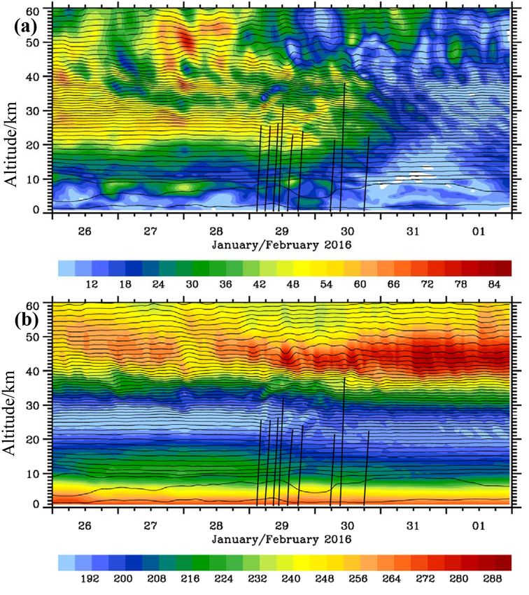
zontal divergence is not spectrally filtered and contains con- Figure 7. Altitude–time sections of the vertical wind w in m s−1
tributions from all resolved wavenumbers. Therefore, indi- (a, 1w = 0.1 m s−1 ) and temperature perturbations T 0 in K (b,
vidual wave groups cannot easily be separated and the DIV 1T 0 = 2 K) as a composite of 1-hourly short-term HRES forecasts
patterns are not directly comparable to the VHIGW field of the and 6-hourly operational analyses from the IFS cycle 41r2 above
Kiruna, Sweden. Positive and negative values are plotted with red
scale-dependent modal decomposition.
and blue lines. The temperature fluctuations are calculated rela-
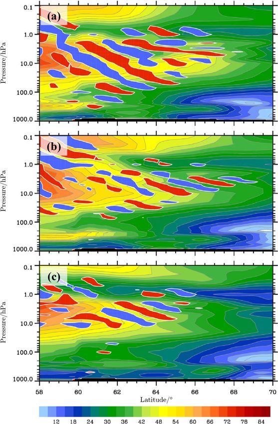
Figure 6 shows the temporal evolution of the zonal com- tive to an area mean. In panel (a), minimum and maximum w val-
ponents U IGW and VHBAL plotted as vertical cross sections ues are −1.5 and 1.2 m s−1 and in panel (b) minimum and maxi-
along the black line drawn in all panels of Figs. 4 and 5. The mum T 0 values are ±15 K, respectively. The thin black lines are the
comparison of the three consecutive analysis times (00:00, logarithm of the potential temperature with constant increments of
06:00, and 12:00 UTC) clearly shows a gradual decrease in 0.05. The vertical black lines mark the radiosonde paths of the nine
the stratospheric winds VHBAL over northern Scandinavia due soundings mentioned in the text.
to the southward displacement of the polar vortex during the
minor SSW. At the northern (inner) edge of the polar vor-
tex inclined phase lines are visible in the U IGW fields and and 2 hPa (Fig. 6c). Altogether, the three snapshots indicate
indicate the gravity waves extracted from the normal-mode a highly transient wave progression at the inner edge of the
analyses. At 00:00 UTC, gravity waves with a vertical wave- polar vortex.
length of about λz ≈ 13 km (estimated from the difference in
Z between 3 and 30 hPa at 62◦ N) dominate the field in south- 5.3 Altitude–time sections
ern Scandinavia (Fig. 6a). These waves are most likely re-
lated to the mountain waves visible in the lower stratosphere Figure 7 presents the two quantities from the IFS simula-
between 60 and 62◦ N. The increase in vertical wavelength tions, delineating gravity wave signatures as a function of
with altitude is in accordance with linear wave theory as time and altitude over Kiruna, Sweden. Plots like Fig. 7 map
λz ∼ U/N . Further south, the upper branch of the wave train the time-dependent 3-D meteorological data into a 2-D view
excited over Scotland is seen above 10 hPa at 06:00 UTC as often provided by ground-based observations of vertical
(Fig. 6b). At the same time, a packet of gravity waves with profilers (Dörnbrack et al., 2017b). Whereas the tempera-
λz ≈ 4–5 km is located at the polar-night jet’s northernmost ture fluctuations originate from a prognostic IFS variable,
tip. It is this wave train we suggest to be excited by spon- the vertical wind is a diagnostic quantity and it is used in a
taneous adjustment in the divergent region of the PNJ. The similar way as the horizontal divergence to visualize gravity
altitude at which the waves appear in the results of the modal waves. Between 26 and 29 January 2016, four sequences of
decomposition is at about 10 hPa (∼ 28 km). The vanishing vertically deep-propagating gravity waves appear as stacked
wave signature above about 3 hPa (∼ 39 km) is consistent positive and negative vertical velocity patterns extending to
with the decreasing wind above this altitude (Figs. 2a, 5b, the upper stratosphere and mesosphere (Fig. 7a). Possible
and 6b). At later times, the waves disappeared above north- sources of these waves could be the weak cross-mountain
ern Scandinavia, whereas only waves with longer vertical flow or the tropopause jet; compare the times of the VH
wavelengths seem to be trapped inside the PNJ between 20 maxima in Fig. 2a with the appearance of the stratospheric
Atmos. Chem. Phys., 18, 12915–12931, 2018 www.atmos-chem-phys.net/18/12915/2018/A. Dörnbrack et al.: Stratospheric excitation of inertia-gravity waves 12925
Table 3. IFS results as in Tables 1 and 2 for the period from 26 Jan- 5.4 Wavelet analysis of the altitude–time sections of the
uary until 1 February 2016. IFS data above Kiruna
26 January–1 February 2016 IFS 2-D wavelets as introduced in Sect. 2 are applied to quan-
EPmw
up
EP EPdown R IFS EPtot tify the stratospheric gravity wave activity and to deduce
potential gravity wave sources as demonstrated by Kai-
1–8 km fler et al. (2017). To classify the dominant vertical prop-
12–20 km 0 1 1 0.45 1 agation directions of gravity waves, contributions from
20–28 km 0 1 1 0.50 3
quasi-stationary waves (mountain waves, ground-based ver-
30–38 km 2 10 6 0.57 20
tical phase speed |cPz | ≤ 0.036 m s−1 ), upward-propagating
40–48 km 0 9 2 0.76 13
waves (cPz < −0.036 m s−1 ), and downward-propagating
waves (cPz > 0.036 m s−1 ) with vertical wavelengths λz be-
tween 2 and 15 km are separated and analyzed independently.
Total potential energy densities EPtot and EP values for the
gravity waves in Fig. 7a. Afterwards, from 29 January at three wave classes are derived and listed as averages over
noon to 30 January at midnight, the simulated stratospheric different altitude layers and for selected periods in Tables 1,
vertical wind patterns are not tied to the troposphere and 2, and 3. Averaging over the entire period from 26 January
tropopause region at this location. Furthermore, the smaller to 1 February, low EPtot values of 1 and 3 J kg−1 are found
amplitudes suggest another excitation mechanism compared below 28 km compared to large values of 20 and 13 J kg−1
to the waves appearing in the preceding days. Apparently, above 30 km of altitude. Altogether, the dominant contribu-
the simulated waves disappeared above 50 km of altitude tions above 30 km of altitude are due to upward-propagating
concurrently with the ceasing horizontal wind after 29 Jan- gravity waves, whereas contributions from quasi-stationary
uary 00:00 UTC; see Fig. 2a. The nine balloon trajectories waves are negligible (Table 3). On 29 January 2016, a strong
as displayed in Fig. 7 indicate that only the deep sounding enhancement of downward-propagating waves is found in the
of the radiosonde launched in Kiruna on 30 January 2016 whole column between 12 and 48 km of altitude (see large
at 09:08 UTC partially penetrated the coherent stratospheric EPdown values in Table 2). Below 38 km, EPdown values clearly
up
wave pattern above 25 km of altitude near the end of the surpass EP values and attain maximum values of 25 J kg−1
regime transition. between 30 and 38 km of altitude. Above 38 km of altitude,
up
The temperature perturbations T 0 were derived relative to EP > EPdown indicates wave generation at around that level
an area mean as described in Sect. 2. The altitude–time sec- in accordance with the ascending and descending phase lines
tion of T 0 as shown in Fig. 7b delineates the very same grav- in Fig. 7b. On 30 January 2016, upward-propagating grav-
ity wave sequences as visible in the vertical wind in Fig. 7a. ity waves dominate the EP values at all altitude bins again.
Here, we relate the direction of the main axis of the elliptical Note that the stratospheric values of EPtot from the IFS agree
patterns of positive or negative T 0 values to phase lines indi- well quantitatively with the EP estimates from the radiosonde
cating the vertical direction of ground-based phase propaga- and reflect the same altitude dependence. For the IFS data,
tion. This is in contrast to altitude–distance plots, in which the ratio of upward-propagating waves to all wave modes is
up up
the phase lines are normal to the direction of phase prop- calculated by R IFS = EP /(EPmw + EP + EPdown ) and R IFS is
agation (Sutherland, 2010, Fig. 1.25). For the sequences of listed in Tables 1 to 3. A comparison with the radiosonde
gravity waves until 28 January 2016, the absolute T 0 val- sounding data reveals both R RS and R IFS values larger than
ues increase up to 15 K in the upper stratosphere. The de- 0.6 for altitudes above 20 km, indicating a dominance of
clining phase lines apparently suggest nonsteady, upward- upward-propagating waves on 30 January 2016. In contrast,
propagating gravity waves. This first qualitative interpreta- the strongly reduced R IFS values between 12 and 38 km on
tion is based on linear wave theory in which downward phase the day before clearly signify the dominance of downward-
propagation is associated with upward energy propagation. propagating modes.
However, the most striking feature of Fig. 7b is the occur- Temperature fluctuations T 0 associated with upward-
rence of ascending phase lines below about 35 km of altitude and downward-propagating waves as separated by the 2-
during 29 January 2016. Linear wave theory suggests down- D wavelet analysis are displayed as vertical time series
ward energy propagation for this period. The signature of this in Fig. 8. Enhanced upper stratospheric T 0 values associ-
highly transient event fades on 30 January 2016. Afterwards, ated with upward-propagating waves persist before and dur-
smaller-scale waves with lower amplitudes are observed fol- ing the regime transition but their amplitude decreases on
lowing the morning of 31 January 2016 after the regime 30 January 2016 (Fig. 8a). Large amplitudes are reached dur-
transition. In order to elucidate upward- and downward- ing 28 January 2016 with vertical wavelengths λz of 10 to
propagating wave components quantitatively, we next apply 15 km. A similar pattern but of weaker amplitudes is found
the 2-D wavelet analysis to the temperature fluctuations T 0 for downward-propagating waves around the same time
shown in Fig. 7b. (Fig. 8b). However, a downward-propagating wave packet
www.atmos-chem-phys.net/18/12915/2018/ Atmos. Chem. Phys., 18, 12915–12931, 201812926 A. Dörnbrack et al.: Stratospheric excitation of inertia-gravity waves
Figure 8. Temperature fluctuations associated with (a) upward- and (b) downward-propagating gravity waves as reconstructed by wavelet
analysis (see text).
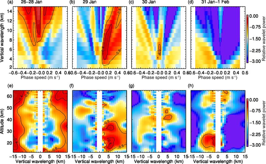
dominates during the regime transition on 29 and 30 Jan- scales of λz ≈ 3 km are found in the lower stratosphere at
uary 2016. It has significantly smaller vertical wavelengths, around 20 km of altitude (Fig. 9d, h).
a larger tilt, i.e., a higher phase speed, and is confined to the
altitude range from 20 to about 45 km (Fig. 8b). The inter-
mittent appearance of downward-propagating stratospheric 6 Discussion and summary
wave packets points to spontaneous adjustment as a possible
generation mechanism in this short time period at the begin- In this paper, we analyzed upper stratospheric gravity waves
ning of and during the regime transition. that occurred at the inner edge of the Arctic polar vortex dur-
The distribution of gravity wave parameters is visualized ing a minor SSW at the end of January 2016. The gravity
in Fig. 9, in which wavelet spectrograms are displayed as waves were observed by a singular radiosonde launched from
a function of vertical wavelength λz , ground-based phase Kiruna airport, reaching an altitude of 38.1 km. This unusual
speed cPz , and altitude for four consecutive time periods. We peak altitude could be achieved first by using a large 3000 g
show relative wavelet spectrograms (see Sect. 2) in order to balloon. Second, the warming of the middle stratospheric
emphasize differences before, during, and after the regime cold layer from 180 to 190 K helped maintain the elastic-
transition due to the minor SSW on 29 and 30 January 2016. ity of the rubber skin until the balloon burst, probably due
The highest value zero means that the wave packet in ques- to strong turbulence. This 10 K warming was associated with
tion was detected in the selected interval only. The wave the southward displacement of the Arctic polar vortex. This
field is dominated by mostly upward-propagating waves with means that the stratosphere above Kiruna was characterized
|λz | ≥ 10 km and negative phase speeds cPz ≤ −0.05 m s−1 by a distinct temporal change in the ambient flow conditions
until 28 January 2016 (Fig. 9a, e). A slightly weaker wave during the period from 29 to 30 January 2016: the warming
with |λz | ≈ 8 km and larger negative phase speed cPz ≤ and descent of the cold stratospheric layer went along with a
−0.17 m s−1 is superimposed. The occurrence of downward- gradual decrease in the horizontal winds during this regime
propagating waves with cPz ≈ +0.17 m s−1 and λz ≈ 4 km transition from vortex edge to center conditions (Fig. 2).
on 29 January 2016 is clearly visible in Fig. 9b. Figure 9f In agreement with previous observational studies (e.g.,
shows their vertical extent between 12 and 40 km of alti- Whiteway et al., 1997; Yoshiki et al., 2004), significant
tude. Simultaneously, upward-propagating waves with λz = stratospheric wave activity could be detected in the high-
5–10 km are found above 40 km of altitude. This promi- resolution IFS data at times when the PNJ was situated over
nent dipole structure indicates a local gravity wave source Kiruna (cf. Figs. 2a and 7a, b), i.e., before and during the
at about 40 km of altitude (Fig. 9f). The stratospheric gravity regime transition. As shown by Le Pichon et al. (2015) and
wave activity decreases dramatically on 30 and 31 January: Ehard et al. (2018), IFS analyses are a reliable indicator of
a downward-propagating wave packet of λz ≈ 5 km and very stratospheric gravity wave activity up to about 45 km of al-
small phase speed is detected in an altitude range between 40 titude. The most recent increase in the IFS horizontal reso-
and 48 km (Fig. 9c, g). A reconstruction of the downward- lution is especially able to reproduce realistic gravity wave
propagating wave packet with λz = 4.7–6.2 km and with amplitudes in the lower and middle stratosphere (Dörnbrack
cPz ≈ +0.1 m s−1 is shown in Fig. 10. Finally, starting on et al., 2017a). The IFS analyses and HRES short-term fore-
31 January, small-amplitude upward-propagating waves with casts suggest that these stratospheric gravity waves were oc-
curring whenever the tropopause jet was located over Kiruna
Atmos. Chem. Phys., 18, 12915–12931, 2018 www.atmos-chem-phys.net/18/12915/2018/You can also read