The Garnaut Reviews' Omissions of Material Facts
←
→
Page content transcription
If your browser does not render page correctly, please read the page content below
The Garnaut Reviews’ Omissions of Material Facts

                                            Timothy Curtin1

"It is a capital mistake to theorize before one has data. Insensibly one begins to twist facts to
suit theories, instead of theories to suit facts." Sherlock Holmes (aka Arthur Conan Doyle)

Preamble

In 1853-54 there was a serious outbreak of cholera in London‟s Soho district. The prevailing
view of scientists at the time was that cholera - like climate change now - was caused by an
invisible miasma in the air, and the Ross Garnauts of that time all deferred to various Royal
Societies (e.g. the Royal College of Physicians) as the definitive authorities. John Snow, a
doctor who had pioneered the use of chloroform, in 1849 published at his own expense the
first book to challenge the conventional wisdom of the authorities of the day, and was duly
put down by them.2 However Snow persevered, and showed how the incidence of cholera in
the 1854 outbreak was closely correlated with the nature of the drinking water supplied by
the Southwark and Vauxhall water company on the one hand, and the Lambeth company on
the other. He eventually won acceptance for his contention that cholera is a water-borne
disease, having shown statistically how most cholera deaths occurred in premises taking their
water from the first company, which had its water intakes adjacent to sewerage outlets to the
Thames, while very few deaths occurred in premises whose water was supplied by the
Lambeth company, which in 1849 had moved its uptake up river from the sewerage outlets.

Snow‟s pioneering counterfactual analysis has recently been cited in two econometrics
textbooks (Angrist and Pischke 2009, Freedman 2010) that explain how multi-variate
regression analysis can be used to evaluate competing theories of causation.34 This paper
shows how such analysis reveals that changes in atmospheric water vapour are a much more
powerful explanation of climate change than changes in carbon dioxide levels, because like
Snow it uses counterfactuals to show that although the atmospheric concentration of carbon
dioxide is ubiquitous (the same everywhere), temperature changes are not, and that in most
places changes in atmospheric water vapour have a very much larger – and much more
statistically significant – association with changes in temperature . Were he alive now it seem

1
  No affiliation (retired), email:tcurtin@bigblue.net.au.
  On the mode of communication of cholera. “Journals dismissed Snow's book - „There is, in our view, an entire
2

failure of proof that the occurrence of any one case could be clearly and unambiguously assigned to water‟.
However the reviewer later concludes, „Notwithstanding our opinion that Dr Snow has failed in proving that
cholera is communicated in the mode in which he supposes it to be, he deserves the thanks of the profession for
endeavouring to solve the mystery. It is only by close analysis of facts and the publication of new views, that we
can hope to arrive at the truth‟". (London Medical Gazette, 1849).Source: www.johnsnowsociety.org
3
  Angrist, J.D. and J-S Pischke (2009). Mostly harmless econometrics: an empiricist’s companion. Princeton
UP, Princeton and Oxford.
4
  Freedman, David A. (2010). Statistical Models and Causal Inference. CUP, Cambridge (see Chapter two:
“Statistical Models and Shoe Leather” for a full account of Snow‟s work).

                                                                                                                1
more than likely John Snow would have been as sceptical of airborne carbon dioxide being
the cause of changing climate everywhere as he was of miasmic air being guilty of spreading
cholera.
Ross Garnaut‟s Update 5 The Science of Climate Change is notable for its avoidance of
econometrics and counterfactuals, and concludes (in its section 4.2.2) by invoking the
authority of the Royal Society, the National Academies of Sciences (USA), and the
Australian Academy of Science with their support for the findings of the International Panel
on Climate Change that global warming is caused by airborne carbon dioxide. In an uncanny
repeat of the views of the peak authorities in 1850, the IPCC‟s Climate Change 2007.The
Physical Science Basis goes out of its way (Solomon et al. 2007:28) to dismiss any role in
climate change for the emissions of water vapour that are simultaneous with emissions of
carbon dioxide whenever there is combustion of hydrocarbon fuels. Yet basic chemistry and
physics show that while water vapour emissions are only in the range of 30-50 per cent of
CO2 emissions by weight, in addition to any moisture content of the fuel, their effect on
surface temperature is much larger (see below). It follows that the tax on carbon to be
proposed by Garnaut‟s next Update paper (17th March 2011) will also be a tax on water
vapour and thereby, unavoidably, on rainfall. The political implications of that remain to be
played out, but it is characteristic of all the Garnaut work on climate change that it dwells
only on the supposed external costs of hydrocarbon combustion and never mentions the
demonstrably larger benefits of elevated atmospheric carbon dioxide and rainfall on the
world‟s primary production.
Statistics and the Garnaut Reviews
Garnaut‟s The Science of Climate Change is the fifth in his series of 8 papers updating The
Garnaut Climate Change Review (2008), but like its predecessors is notable as much for what
it leaves out as for what it thereby tendentiously includes. The list begins with Garnaut‟s first
“key point”:
Observations and research outcomes since 2008 have confirmed and strengthened the position
that the mainstream science then held with a high level of certainty, that the Earth is warming
and that human emissions of greenhouse gases are the primary cause. ..The statistically
significant [sic] warming trend has been confirmed by observations over recent years: global
temperatures continue to rise around the midpoints of the range of the projections of the
Intergovernmental Panel on Climate Change (IPCC) and the presence of a warming trend has
been confirmed [sic].
However, the paper Global Temperature Trends by Breusch and Vahid (2011) commissioned
by Garnaut for his 2008 Review, and updated for his new review, does not provide a great
deal of support for that “statistically significant warming trend” being attributable to miasmic
carbon dioxide.5
5
Garnaut No5 (2011) states “I asked two leading econometricians (Trevor Breusch and Farshid Vahid),
respected authorities on the analysis of time series, to examine the temperature record from the three (sic)
authoritative global sources”, failing even to mention the existence of the more comprehensive satellite data sets
(UAH and RSS). Breusch and Vahid also failed in their primary duty of due diligence by remedying Garnaut‟s
refusal to admit the existence of satellite records by checking them anyway.
2We conclude that there is sufficient statistical evidence in the temperature data of the past 130-
160 years to conclude that global average temperatures have been on a warming trend. The
evidence of a warming trend is present in all three of the temperature series. Although we have
used unit roots and linear trends as a coordinate system to approximate the high persistence and
the drift in the data in order to answer the questions, we do not claim that we have uncovered the
nature of the trend in the temperature data. There are many mechanisms that can generate trends
and linear trends are only a first order approximation… It is impossible to uncover detailed trend
patterns from such temperature records without corroborating data from other sources and close
knowledge of the underlying climate system.
Their first statement depends heavily on the absence of the tropics from global temperature
sets for the period between 1850 and 1910 (see my Fig.2), as it was not until the 1950s that
global temperature becomes a valid statistic, for only then did global surface temperature
coverage reach 80 per cent, and it is now below that level again. This makes it very strange
that Breusch and Vahid (2011) never assess the trends in the more truly global satellite
temperature data sets, which surely should “corroborate” their data even though they do not
go further back than 1978. The truth is shown in Fig.3: the linear trend in the UAH satellites‟
global data from December 1978 to February 2011 has an R 2 of 0.345, which is well below
the minimum for statistical significance of 0.5, and indicates a rise of 0.0012 oC per month
since 1978, or 0.0144 p.a., 0.144 per decade, and 1.44oC per century, well below the 3oC
predicted by the IPCC, let alone the 5oC predicted for 2100 by Garnaut (2008:Fig.4.5) if there
is no “mitigation” (i.e. reduction of projected Business as Usual emissions, BAU). The
UAH data do not in fact “corroborate” the NASA-Gistemp temperature data for the period
when they overlap, as the latter shows a very large and apparently statistically significant
trend since 1978 (see my Fig.4), with the annual change in the Gistemp series (1979-2010) at
0.0196oC, which is 36 per cent higher than the UAH trend of 0.0144 oC.
Ross Garnaut like myself worked on the very successful float of Lihir Gold on the Australian
Stock Exchange (ASX) in 1995 (in his case for Rio Tinto and in mine for the Government of
Papua New Guinea). As he and I both know well, a prospectus like that for Lihir is required
by the ASX rules for “Initial Public Offerings” not to leave out any material information with
respect to the company being floated. In particular, “a prospectus is required to contain all
the information that investors and their advisers would require and expect to make an
informed assessment of the offer being made”, ASX, 2011, my emphasis).
Garnaut‟s 8 Update Reports and 2008 Review are both in the nature of a Prospectus, inviting
the Government and people of Australia to invest in a Carbon Tax (and eventual Emissions
Trading Scheme, ETS) that will save them the costs of “dangerous climate change”. That
means Garnaut‟s 2008 and 2011 reviews should have disclosed the UAH satellite data as well
as the Gistemp/NCDS/HadleyCRU surface data, even if using the former would have diluted
the all too evident advocacy that characterises the Garnaut reviews.
Not even to mention the satellite data, and instead relying on surface measurements that
perforce did not include the tropics before 1910, is again to omit “all the information that
investors and their advisors would require and expect” to find in a company‟s IPO
prospectus. The prospectus of a company that mentions only its profitable years and leaves
out years of losses is very like the Hadley CRU, NCDC, and NASA-GISS data for “global”
temperatures for 1850 to 1910 which omit the globe‟s hottest places, like Khartoum,
Kampala, and Kinshasa (see my Fig.2), but are relied on by Garnaut‟s Breusch and Vahid for
the baseline they need to show “unprecedented warming” since 1850 or 1880, see their Fig.1.
3However, there is a much more serious omission of “all the information investors and their
advisors would require and expect” in both the Garnaut Reviews when they make this
statement:
No-mitigation case – based on no action undertaken to mitigate climate change, and used as a
„reference‟ to assess the benefits of climate change action that accrue from the climate change
impacts that are avoided. By the end of the century the concentration of long-lived greenhouse
gases in the atmosphere is 1565 ppm carbon dioxide equivalent (Garnaut 2011:5 and Fig.1, my
emphasis).
The present atmospheric concentration of CO2 is 390 parts per million (ppm) of the
atmosphere. To this Garnaut adds the atmospheric levels of other greenhouse gases, chiefly
methane (CH4) and nitrous oxide (N2O), which are expressed in CO2 “equivalent” amounts
that bring the CO2e concentration to between 455 and 465 ppm in 2010. To get from 460 ppm
to 1565 ppm by 2100 requires that the rate of growth of CO 2e from now until 2100 has to be
1.0137 per cent p.a. The actual growth of atmospheric CO 2 from 1958 to 2010 was 0.295 per
cent p.a., and projecting CO2e at that rate (the growth rates of CH4 and N2O are much lower
than that of CO2, see IPCC, Solomon et al. 2007:141)6 to 2100 produces only 600 ppm of
CO2e by 2100, less than 38 per cent of (i.e. 62 per cent less than) Garnaut‟s 1565 ppm.
Garnaut offers no basis for predicting any acceleration in the rate of growth of the
atmospheric concentration of CO2e above the actual rate from 1958 to 2010, and, failing that,
this claim in his Update 5 paper is equivalent to that of a company like Lihir Gold claiming in
its IPO Prospectus in 1995 that it could borrow at say 1 per cent above LIBOR instead of the
actual 2-3 per cent it did have to pay to its main bank lender, UBS. Had Lihir Gold made that
claim, the ASX might well have rejected the Prospectus –and if not, shareholders would have
been able to sue Lihir Gold when the truth became apparent.
The Real Science of Climate Change 7
Real science involves very precise formulae, like Einstein‟s
E = MC^2 …(1)
or the formula for combustion of a typical hydrocarbon fuel in the presence of air (using pure
oxygen tends to raise the proportion of H2O in the outputs):
C3H8 + 5O2 + 18.8N2 → Energy + 3CO2 + 4H2O +18.8N2 …(2)
Climate science has never produced any such formulae, and as discussed below, always
suppresses the second formula. If it could, we would be presented with something like
C + O2 → CO2 together with ΔHjo= -393.51 kJ plus xW/sq.m…(3)
where C is solid carbon (graphite) and ΔHjo is the standard heat of formation, being the
enthalpy change that occurs when one mole of a substance is formed from its component
6
Growth of the methane concentration from 1998 to 2005 was NIL, despite Garnaut‟s claim (2010) that its
growth rate is increasing, and of N2O, 11 per cent over that period (in total, not p.a.), against 13 per cent in CO2
(IPCC, Solomon et al. 2007:141).
7
This section has benefited considerably from the insights of Anthony Kelly (2010). He notes that in the
various applicable chapters in the IPCC‟s Solomon et al. (2007) no mention is ever made of the fact that most if
not all anthropogenic water vapour is in the form of steam (p.630).
4elements and x is the radiative forcing associated with the replacement of the O2 in the
atmosphere by CO2.
Climate science has never been able to produce such a formula simply because it cannot, as
there is no such precise relationship. The closest climate scientists get to producing a formula
for the “radiative forcing” of greenhouse gases, namely the strength of their ability to radiate
heat back to earth, is their equation 4. The subsequent change in equilibrium surface
temperature (ΔTs) arising from that radiative forcing is given by:8
…(4)
where λ is the assumed (not proven) climate sensitivity, with units in K/(W/m 2), and ΔF is
the assumed radiative forcing, given by
…(5)
where C is the current or future level of atmospheric carbon dioxide and C o is the pre-
industrial level (280 ppm), and F is measured in Watts per square metre. A typical value of λ
is said to be 0.8 K/(W/m2), which gives a warming of 3 oC for a doubling of CO2 (from 280
ppm to 560 ppm). The parameters λ and 5.35 are not data-based, e.g. by use of linear least
squares regression, being fitted ex post at whatever level seems to match the observations
(see Myhre 1998), so the only data in (4) and (5) are the base and projected levels of CO2. 9
As a result, this model consistently overstates its forecast of global temperature from 1959 to
2010 by 0.0112oC p.a. (0.112oC per decade), and 0.59oC for 2010 compared with the
Gistemp global temperature of 14.83oC in that year (see my Fig.8). That is not a trivial
difference, and it gets worse over time.
Thus the equations (4) and (5) may look impressive but they lack the precision of Einstein‟s
(1) or the chemical formulae like (2) that govern the combustion of hydrocarbon fuels. Not
only that, if climate scientists were capable of the basic linear least squares regression
analysis in which Arrhenius (1896) was fully proficient, they would at least be able to do
regressions in which they showed that
ΔTt = a + b(3CO2)t + c(4H2O)t +d(18.8N2)t + ut …(6)
and then provided statistically significant values for the coefficients. But they never have
provided such values for the b and c coefficients like those I show below.
Similarly while climate scientists are aware of the Clausius-Clapeyron relation which defines the
maximum partial pressure of water vapour that can be present in a volume of atmosphere in
thermodynamic equilibrium as a strongly increasing function of temperature, they have failed to
8
This account is based on the article Radiative Forcing in Wikipedia, accessed 14th March 2011.
9
Myhre, G, E.J. Highwood, K.P. Shine, F. Stordal (1998). New estimates of radiative forcing due to well
mixed greenhouse gases. Geophysical Research Letters, 25.4, 2715-2718
5quantify it accurately in the context of their predicted climate change. This maximum is known as the
saturation vapour pressure, es:
es(T) = es(To)exp-L/Rv(1/T-1/T0) ….(7)
“where L is the latent heat of the appropriate phase transition (vapour to liquid at warm temperatures,
vapour to solid at sufficiently cold temperatures), Rv is the gas constant for water vapour, and To is a
reference temperature. At the freezing point, es is 614 Pa or 6.14 mb; L/Rv = 5419 K for condensation
into liquid and 6148 K for condensation into ice” (Pierrehumbert et al. 2007:145).10
It is important to realise that while satellite observations indicate that the response of global
evaporation to rising temperature is close to that implied by (7), with the cooling effect entailed by
evaporation and associated precipitation, the GCM models deployed by climate scientists apparently
reduce the evaporation implied by Clausius-Clapeyron, presumably because it increases potential
global warming (Kininmonth 2010:61).
Pierrehumbert et al. (2007:180) also caution against what they term “wholly indefensible statements
which simply invoke the Clausius-Clapeyron relation…[as being] at the root of the behaviour of water
vapour, but the proper use of the relation hinges on identifying the temperature to which the relation
should be applied; it’s not the surface temperature, and the effect of the relation on evaporation is of
little relevance to water vapour feedback” (my emphasis).
As a result of not acting on the advice of Pierrehumbert et al. (2007), Solomon et al. (2007)
wrongly attribute increases in water vapour only to rising surface temperatures, although
using those increases to raise the radiative forcing they ascribe to atmospheric carbon dioxide
is enough to triple the temperature change due to that by 2100 from 1 oC to 3oC. This artefact
is termed the “feedback” effect whereby rising temperature raises evaporation whose own
radiative forcing would be much stronger than that of atmospheric carbon dioxide alone, were
it not for precipitation rising pari passu with evaporation. But Randall and Wood et al. 2007
in Solomon et al. (2007:633) and Garnaut (2008:81 and 2011:26-27) downplay the role of
precipitation in cancelling out rising evaporation, indeed they predict increasing drought
despite the rising water vapour they rely on for their infinitely spiralling further temperature
increases that deliver their desired “runaway” greenhouse effect.
However, Pierrehumbert et al. (2007) also assume that increases in atmospheric water vapour
(hereafter denoted by [H2O]) stem only from rises in temperature, and are independent of processes
like combustion of hydrocarbons that directly release water vapour into the atmosphere. Such releases
must be more than as potent pro rata– in terms of generating radiative forcing by reducing outgoing
long wave radiation (OLR) - as increases in [H2O] resulting from rising temperature. Moreover, like
those increases in [H2O], the increases produced by combustion must also be “approximately
logarithmic in specific humidity once the [total] concentration is sufficiently large to saturate the
principal absorption bands”. Moreover, “one finds that each doubling of water vapour reduces OLR
by about 6W/m2 (Pierrehumbert 1999). This is about 50% greater than the sensitivity of OLR to CO2.
10
Raymond T. Pierrehumbert, Hélène Brogniez, and Rémy Roca (2007). On the Relative Humidity of the
Atmosphere, chapter 6 in The Global Circulation of the Atmosphere, T Schneider and A Sobel, eds. Princeton
University Press. (2007).
6The idea that small quantities of water vapour can have a lot of leverage in climate change has a fairly
long history, and is now widely recognized. Water vapour feedback was included in the very first
quantitative calculations of CO2-induced warming by Arrhenius [1896], and the importance of water
vapour aloft was implicit in such calculations…” (Pierrehumbert et al. 2007:146).
For example, we know that in 2008-2009 combustion of hydrocarbon fuels generated
emissions of about 8.6 billion tonnes (8.6 GtC) of carbon (or 31.4 billion tonnes of CO2, i.e.
31.4 GtCO2) (le Quere et al., 2010) – and from data in Gaffen and Ross (1999) that implies
direct water vapour emissions (just from the combustion process of burning a hydrocarbon
fuel using oxygen) of 17.5 GtH2O.11 But using the Pierrehumbert et al. figure above, the
radiative forcing (RF) from this addition to [H2O] is 50 per cent higher than that of increased
atmospheric CO2. According to the IPCC (Forster and Ramaswamy 2007: 141), the radiative
forcing per GtCO2 is 0.0019 Watts/sq.metre, so that from changes in [H2O] is 0.0028
W/sq.metre. That means hydrocarbon combustion generated RF of 0.108 W/sq.m. in 2008-
09, of which 0.059 W/sq.m. was due to carbon dioxide emissions, and 0.049 W/sq.m. to
water vapour emissions. Yet Garnaut‟s The Science of Climate Change never notices this
effect, and it is dismissed as of no consequence by the IPCC‟s Forster and Ramaswamy et al.
(2007).
The implications are very profound, because if the IPCC and Garnaut are right that increasing
water vapour does not lead to increased precipitation, then the RF and resulting global
warming from hydrocarbon fuel combustion have been seriously underestimated. However
Lim and Roderick (2009) have shown that in reality, while there is evidence for increasing
evaporation between 1970 and 1999, it has been matched by increased rainfall, pace Garnaut
and the IPCC.12 Thus just as the IPCC and Garnaut generally ignore uptakes of CO 2
emissions by the biospheres, they also ignore that rising [H2O] is matched by rainfall. This
explains why they always ignore the positive social benefits of the output of hydrocarbon
combustion, and explicitly treat increases in agricultural productivity and rainfall as social
“bads”.
Regression analysis of climate science counterfactuals
Using the Mauna Loa data set on addition to atmospheric CO2 from 1958 to 2009, and
regressing Gistemp temperature anomalies against it , we have the results shown in Table1.
11
“Based on carbon emissions data (Marland et al. 1994), we estimate global water vapor emission from fossil
fuel consumption to be of order 1012 (in 1960) to 1013 (in 1990) kg yr−1”, Gaffen and Ross, 1999. Carbon
emissions were 5.57 GtC in 1990, yielding a factor of 5.57/10 for the ratio between emissions of water vapour
and carbon, in Giga tonnes, from hydrocarbon combustion, namely 1.795, say 1.8 (or 0.49 Gt H 2O to 1 Gt of
CO2).
12
Lim, Wee Ho and M.L. Roderick 1999. An Atlas of the Global Water Cycle Based on the IPCC AR4 Climate
Models. ANU E-Press, Canberra.
7Table 1 Regression of Absolute Values of GMT anomalies (as reported by Gistemp)
against [CO2] data (absolute ppm), 1959-2009.
These results look impressive, with a high R 2 of 0.8 and a statistically significant coefficient
on the CO2MLO variable (i.e. atmospheric CO2 as measured at the Mauna Loa Observatory).
But as von Storch and Zwiers note in their textbook (1999), comparison of time series using
least squares regression has a high risk of serial or spurious correlation, and the Durbin-
Watson statistic at 1.666 shows that to be potentially the case in this instance.
This problem is usually addressed by taking year-on-year differences in the data, with the
results shown in Table 2:
Table 2 Regression of changes in surface-measured GMT on changes in [CO2]
Table 2 probably explains why the IPCC (Solomon et al. 2007) and Garnaut (2008 and 2011)
never report regression results, for while the Durbin-Watson statistic at 2.5 rules out serial
correlation, the R2 falls to .317, indicating that the CO2 variable, although statistically
significant, does not account for “most” (i.e. more than 50 per cent) of observed temperature
change since 1958, as claimed by Garnaut (2011), Hegerl and Zwiers et al. (2007:670) and
Solomon et al. (2007:10).
The truth evaded by Garnaut is that Hegerl and Zwiers as lead authors of the crucial Chapter
9 (“Understanding and Attributing Climate Change”) in IPCC‟s AR4 (Solomon et al. 2007)
were well aware that standard multivariate regression analysis of changes in temperature as a
function of changes in atmospheric CO2 and natural influences (e.g. water vapour) does not
8yield their desired outcomes, hence their refusal to report such analysis. Instead they have
resorted to developing a new method of analysis that they have named “detection and
attribution of fingerprints (sic)”. But this system does not appear in standard textbooks, as it
twists the raw data into their desired shapes by use of modelled parameters rather than using
only raw data. Thus although their model has the form y = Xa + u where y is the “filtered”
climate variable and X is a matrix of independent variables that could determine y, while a is
a vector of scaling factors. But in their hands X, the matrix for the independent variables,
contains only “signals that are estimated” by climate models, rather than real world data
(Hegerl and Zwiers et al. 2007: 744).
Thus their model is tautologous, as by avoiding use of data it always delivers the pre-
determined results generated by its climate models. Nevertheless, Francis Zwiers was invited
to give testimony to the United States‟ House of Representatives Committee on Energy and
Commerce, Subcommittee on Energy and Power hearing entitled “Climate Science and
EPA‟s Greenhouse Gas Regulations” on 8th March 2011. Here is a direct quote from Zwiers‟
Testimony: “Figure 2 also shows the prediction that was made by the IPCC in 2001 that the
decade of the 2000s would be 0.1-0.2oC warmer than the 1990s, primarily because of the
influence of rising greenhouse gases” – but fails to provide any statistical evidence linking
that 0.1-0.2oC to rising atmospheric CO2. It is telling that his Figure 2 does not include the
linear regression trend lines for the temperature data used there, as they are of course
derisory, even though naturally he uses 2000, a La Nina year as his start year:
y = 0.0015x + 0.151
R² = 0.1073
(UAH Global temperature anomalies January 2000 to October 2010; I left out the very cold
La Nina-affected November and December 2010 just to be helpful to Zwiers).
Zwiers similarly chose not to show the trends in increases in the atmospheric concentration of
CO2 for 2000 to 2010, perhaps because the trend is actually slightly negative (albeit not
significantly so) for that period:
y = -0.0035x + 1.998
R² = 0.0009
Comparison of these two trends may explain why Zwiers like Garnaut does not perform
regressions on his data. Here are the results:
(1) Constant = 0: UAH anomalies = f(increases in CO2)
Adj R2: 0.014; Coeff. on CO2= 0.035; t = 1.68; p = 0.096
(2) Constant not zero:
Adj R2: 0.0004; Coeff. on CO2= 0.0116; t = 0.97; p = 0.33
Setting the constant (y-intercept) at zero gives Zwiers his best chance, but it does not help. In
both cases there is NO statistically significant correlation at all between the increases in CO 2
9and the UAH anomalies (for that the t statistics should be >2, the p < 0.15, and the R2 should
be at least 0.5). However if Zwiers had regressed sales of mobile phones against atmospheric
carbon dioxide data he would doubtless have found a stunning correlation.
John Snow’s Counterfactuals, Carbon Dioxide, and Climate Change
In the Preamble I gave a brief account of John Snow‟s counterfactual analysis of cholera by
collecting statistics on the distribution of sources of water supply by households and of deaths
from cholera. The problem with the bivariate regressions of global temperature change and
atmospheric carbon dioxide reported in the previous section is that the only independent
variable is changes in atmospheric CO2. In that regard such regressions are like those
implicitly relied on by the medical establishment in London in 1854, which could as easily
have proved that the increasing incidence of cholera outbreaks was due to the equally well
attested increase in use of horse-drawn vehicles, omnibuses, cabs, and the carriages of the
rich, with horses‟ exhalation a plausible source of the miasma passionately believed by the
Garnaut reviews of the day to be the cause of cholera.
The modern equivalent of John Snow‟s careful mapping of cholera deaths and water supply is
climate data sets from over 1200 locations produced by the US Government‟s NOAA13 that
are deliberately ignored by the climate change establishment and its cheerleader, Ross
Garnaut along with Breusch and Vahid, seemingly because they include time series of a wide
range of climatic variables, not just temperature.
These location-specific and multivariate data sets provide counterfactuals simply because
although atmospheric carbon dioxide is known to be a “well-mixed” greenhouse gas (i.e.
WMGHG), like London‟s miasma in 1854, which means it is at much the same level
everywhere, from Point Barrow in Alaska to Cape Grim in Tasmania to Mauna Loa in
Hawaii, temperature trends are NOT the same everywhere, and are in general more closely
associated with other climatic variables, such as the amount of sunlight reaching the surface,
and, above all, the level of atmospheric water vapour, i.e. [H2O]. In Fig.5 and Fig. 6 below
the trends in annual mean maximum, minimum, average daytime, and mean temperatures are
shown for both Point Barrow in Alaska and Hilo (near Mauna Loa) in Hawaii for the period
1960-2006. The respective trends differ considerably, although the R 2 correlation coefficients
do not suggest high statistical significance. The nil trends in annual mean temperature at
Honolulu and Mauna Loa itself from 1978-2006 (Fig.7) with R2 of 0.01 and 0.1 respectively
contrast with that for atmospheric carbon dioxide (R 2 0.99) (time series determined by data
availability), and explain the poor correlations.
Regression analysis of the NOAA climate data for Pt Barrow for 1960 to 2006 (when this set
terminates) provides a striking example of John Snow‟s counterfactual analysis. As shown in
Table 3, changes in the level of atmospheric carbon dioxide play no role at all in explanation
of the significant warming trend in minimum temperatures, while the role of atmospheric
water vapour [H2O] is strong and very highly significant (99%), along with opacity of the sky
13
http://rredc.nrel.gov/solar/old-data/nsrdb/1961-90/dsf/data and http://rredc.nrel.gov/solar/old-data/nsrdb/1991-2005/statistics/data
10at night (OPQ). Similar results are found for various locations in Hawaii, such as Hilo (Table
4), and New York City (Table 5), and many others, not reported here for reasons of length.
These counterfactuals all show no statistically significant correlations between atmospheric
carbon dioxide levels (i.e.[CO2]) and changes in temperature, and thereby fully support the
conclusions of Paulo Cesar Soares (2010:111), that there is no causal relation between [CO2]
with global warming, given the absence of evidence for changes in [CO2] preceding
temperature either for global or local changes, and that the greenhouse effect of [CO2] is
very small compared with that of water vapour.14
Table 3 Regression of climate data, P Barrow 1960-2006
SUMMARY OUTPUT
Dependent variable: Mean minimum annual temperatures,
Pt Barrow 1960-2006
Regression Statistics
Multiple R 0.78
R Square 0.60
Adjusted R Square 0.57
Standard Error 1.04
Observations 46.00
ANOVA
df SS MS F
Regression 3 69.02 23.01 21.16
Residual 42 45.67 1.09
Total 45 114.69
Coefficients Standard Error t Stat P-value
Intercept -0.05 0.40 -0.12 0.91
H2O 13.64 2.75 4.96 0.00
CO2 ML 0.02 0.26 0.06 0.95
OPQ 1.20 0.29 4.19 0.00
Independent variables
H2O = atmospheric water vapour
CO2 ML = atmospheric CO2
Sources: http://rredc.nrel.gov/solar/old-data/nsrdb/1961-90/dsf/data and http://rredc.nrel.gov/solar/old-data/nsrdb/1991-
2005/statistics/data
14
P.C. Soares 2010, Warming Power of CO2 and H2O: Correlations with temperature changes. International
Journal of Geosciences, 102-112.
11Table 4 Multivariate regression of climatic variables, Hilo 1960-2006
SUMMARY OUTPUT
Dependent variable: Changes in Annual Maximum Temperature
Hilo, Hawaii 1960-2006
Regression Statistics
Multiple R 0.59
R Square 0.35
Adjusted R Square 0.28
Standard Error 0.59
Observations 45
ANOVA
df SS MS F
Regression 4 7.46 1.87 5.38
Residual 40 13.86 0.35
Total 44 21.32
Coefficients Standard Error t Stat P-value
Intercept 0.13 0.24 0.54 0.59
dCO2 -0.07 0.16 -0.47 0.64
dAVGLO 0.00 0.00 3.34 0.00
dAvWS -0.09 0.34 -0.27 0.79
dH2O 2.35 0.58 4.08 0.00
Independent variables
dCO2 = annual changes in atmospheric carbon dioxide at Mauna Loa Slope Observatory;
dAVGLO = Average daily total solar radiation, i.e. sum of direct and diffuse radiation less
albedo (Wh/m2);
dAvWS = Changes in annual average wind speed;
dH2O = changes in precipitable water vapour (cm).
Sources: http://rredc.nrel.gov/solar/old-data/nsrdb/1961-90/dsf/data and http://rredc.nrel.gov/solar/old-data/nsrdb/1991-
2005/statistics/data
12Table 5 Regression of climate data, New York City (JFK) 1960-2006
SUMMARY OUTPUT
Dependent variable: mean annual minimum temperature
New York 1960-2006
Regression Statistics
Multiple R 0.85
R Square 0.72
Adjusted R Square 0.69
Standard Error 1.86
Observations 46
ANOVA
df SS MS F
Regression 3 365.79 121.93 35.15
Residual 42 145.69 3.47
Total 45 511.49
Coefficients Standard Error t Stat P-value
Intercept -0.26 0.67 -0.39 0.70
dCO2 0.06 0.43 0.14 0.89
dH2O 18.64 1.93 9.64 0.00
dOPQ -0.53 0.35 -1.49 0.14
dOPQ = average annual opacity of sky cover.
Sources: http://rredc.nrel.gov/solar/old-data/nsrdb/1961-90/dsf/data and http://rredc.nrel.gov/solar/old-data/nsrdb/1991-
2005/statistics/data
The Benefits of Hydrocarbon Fuel Emissions
Garnaut‟s first Update paper (2011) has the title “Weighing the costs and benefits of climate
change action”, and like the fifth is in breach of ASX disclosure rules, because at no point
does it mention the undoubted benefits of hydrocarbon combustion in terms of (1) the
fertilization effect of elevated atmospheric carbon dioxide on primary production, and (2) the
benefits in terms of enhanced crop yields of higher global rainfall. For Garnaut (2008 and
2011), hydrocarbon combustions produce only costs, in the form of as yet unproven large
rises in global mean temperatures (even though they would also have benefits in the form of
13higher crop yields in all higher latitude zones), and the benefits of restricting use of
hydrocarbons consist only of avoidance of the supposed costs of rising temperatures.15
Ironically, there is a huge contradiction between the basic Garnaut position that hydrocarbon
emissions produce only costs, while in both his 2008 and 2011 reviews, he devotes space to
the role of expanding agro-forestry in order to reduce atmospheric carbon dioxide
concentrations through their absorption of substantial volumes of those emissions. In the
2008 Review Garnaut was able to raise the historic growth rate of the concentration of CO2e
at 0.29 per cent p.a. (1958-2010) to his projection of 1.0137 per cent p.a. from 2010 to 2100
by suppressing the known take-up of more than half of carbon dioxide emissions by the
globe‟s biospheres (Knorr 2009). He justifies that in his Update 5‟s section 2.3.2 on the
carbon cycle which at face value seems unexceptionable but nevertheless displays palpable
bias. The first is the stress on the apparently fast growth of fossil fuel emissions between
2000 and 2008 of 3.4 per cent p.a., without mentioning that in that period the atmospheric
concentration of carbon dioxide increased by only 0.296 per cent p.a.
This distinction between the respective growth rates of emissions and of the atmospheric
concentration is very important but never mentioned either in Garnaut 2008 or in the 2011
Update, and betrays some ignorance of dependence of percentages on respective base levels.
Total annual emissions of human-generated carbon dioxide are approaching 10 billion tonnes
of carbon-equivalent CO2 (i.e. GtC), but the absolute atmospheric concentration is nearly 830
GtC. An increase of three percent in the first figure, of which over half is absorbed by the
biospheres, becomes just 0.02 per cent of the second figure.16
At the observed atmospheric concentration growth rate of 0.295 per cent p.a. over the longer
period from 1959 to 2009, it will take until 2134 for the so-called pre-industrial level of the
atmospheric concentration of 280 ppm to double to 560 ppm; and the 2009 level of 387 ppm
will not double until 2244. The Review‟s portrayal of the extreme urgency of preventing
these gentle increases is not compelling, unless one accepts the Garnaut projection of 1565
CO2e by 2100.
Update 5 justifies its alarmism by claiming that the strength of the carbon sinks (which have
on average absorbed 56 per cent of carbon dioxide emissions since 1958) has been
“declining” over the last five decades, which if true would result in an increasing airborne
fraction of emissions from the present average level of 44 per cent p.a. It offers no statistical
evidence beyond its repeated citations of papers by J.P. Canadell, C. Le Quere, P. Fraser, and
M. Raupach, of which none of those cited in section 2.3.2 has been peer-reviewed. Instead in
another omission of material facts, Update 5 ignores the peer-reviewed paper by W. Knorr
15
This is an unusual form of cost benefit analysis, pioneered by Stern (2007), whereby the cost of one course of
action is the benefit if that course of action if not adopted. Normally, costs and benefits should be independent
of each other, not one and the same.
16
Garnaut (Melbourne Institute, 20th May 2010) joined the 21 leading Australian economists led by John
Quiggin who by endorsing the Rudd government‟s proposed Resource Super Profits Tax (2010), accepted the
Henry Tax Review‟s claim (2010) that the existing company tax rate of 30% of taxable profits and the average
State royalty rate of 5% of sales revenue were by 2009 generating tax receipts of only 17% of taxable profits -
truly a case of New Political Arithmetic.
14(2009) in a mainstream journal, which concludes “despite the predictions of coupled climate- carbon cycle models, no trend in the airborne fraction can be found”.17 A peer-reviewed paper that appeared in the same month as Knorr‟s provided substantive statistical support for the benefits conferred on mankind by the rising level of atmospheric carbon dioxide through its enhancement of the photosynthesis on which all living matter is wholly dependent.18 That “externality” is never mentioned in Garnaut 2008 and 2011 even when admitting that expanding agro-forestry can increase the uptakes of carbon dioxide emissions that elsewhere he projects as falling to nil (2008: Fig.2.7). The role of Temperature and CO2 in raising photosynthesis – and thereby yields – is shown in Fig.1. Evidently the more CO2 is available at any given temperature the higher is the net primary productivity (NPP). Similarly, the higher the temperature at any level of CO2, the higher is the NPP (left axis) up to the limits specified. Combining higher temperature with higher CO2 again leads to higher NPP. We are now at 390 ppm and
Similarly, Table 6 confirms the concurrence in Fig.1 of rising atmospheric carbon dioxide
with rising terrestrial uptakes of carbon dioxide and rising world cereals production both in
total and per capita. The Garnaut Reviews will incur a heavy burden of responsibility if their
efforts to secure a reduction of carbon dioxide emissions succeed in reducing the atmospheric
concentration to levels like that shown for 350 ppm in Fig.1 that are unlikely to support the
food requirements of a world population of nearly 7 billion now and possibly 9 billion by
2050.

                                                     Table 6

                     Carbon Dioxide and World Cereals Production 1961-2007

                                                                   1961                2007   % Increase
 Total Atmospheric Carbon Dioxide GtC                            673.01              815.10          21.11
 Anthropogenic Emissions of CO2, GtC                               4.06                9.94         144.83
 Total Land Uptakes of CO2 emissions, GtC                          0.90                2.98         231.11
 Total cereals output, billion tonnes                              0.88                2.34         167.14
 Carbon content (40%), GtC                                         0.35                0.94         167.14
 Population, billion                                               3.08                6.60         173.00
 Cereals output per capita, tonnes                                 0.28                0.35          24.64
 Carbon content per capita (40%), tonnes                           0.11                0.14          24.64

Source: Le Quéré, Canadell et al. 2009, FAO 2009.

Note: The world‟s uptakes of atmospheric carbon dioxide are not limited to cereals - other
food and fruit crops, livestock, forestry, and fisheries are all contributors.

Conclusion

Ross Garnaut ends his Update 5 with this comment (p.44):

         Scepticism is an essential part of the scientific process and serves to move the science
         towards greater understanding and agreement. Once a theory is put forward by a
         researcher, it is discussed, analysed and criticised by the wider scientific community.
         Further tests, modelling and research then respond to that questioning. The consequent
         exchanges determine whether the initial conclusions hold, need refining or are rejected.

I offer this critique of Garnaut‟s Updates in that same spirit, and look forward to engaging
with Ross Garnaut, but from experience I am doubtful of any response being forthcoming. I
published a detailed peer-reviewed analysis of Garnaut‟s 2008 Review in Quadrant (January
2009), one of Australia‟s only two monthly current affairs magazines, and never received any
response, despite supportive comments from two ministers in the Hawke and Keating
governments and some senior academics. So much for questioning leading to “exchanges”,
but perhaps this time I may elicit some serious evaluation of the rather serious criticisms here
of Garnaut‟s Updates.19

19
     For a critique of Garnaut‟s first Update paper, see Cox and Stockwell (2011).

                                                                                                        16
APPENDIX
Hydrocarbon Taxation – some preliminary comments
Ross Garnaut‟s Sixth update paper Carbon Pricing and Reducing Australia’s Emissions was
published on 17th March 2011. It argues that for Australia to achieve a contribution to a
“moderately ambitious global mitigation effort aimed at limiting the atmospheric
concentration to 550 ppm of carbon dioxide equivalent”, the carbon (sic) tax the Australian
government has announced it will introduce with effect from 1 st July 2012 should be set
within a range of $20-$30 rising at 4 per cent real p.a., until its replacement around 2015 by
an Emissions Trading Scheme with annual reductions in sales of permits based on declining
emissions caps.20
The Update 6 paper has little to say about the charging and collection basis for the tax. For
example, it assumes that with a carbon tax of $20-$30 per tonne of CO2-e and given that 2.29
kilograms of CO2-e are emitted from each litre of petrol (p. 10, footnote 2, citing Grattan
Institute 2010b, unpublished), “the impact on the price of petrol of a carbon price in the range
discussed in this paper would be about 5-7 cents per litre”. It is painfully obvious that this
calculation is set to downplay the impact of the “carbon” tax on pump prices of petrol,
because it ignores the large energy usage of oil refineries, where energy can account for over
72 per cent of operating costs (Stern 2007:301). That energy usage is almost wholly carbon-
based, whether from electricity derived from the grid, which in Australia is heavily dependent
on coal-fired power stations, or from its own fuel oil, which will also like the power stations
be subject to the “carbon” tax.
Thus Garnaut‟s Update 6 ignores that 0.27 kg of CO2 are needed per kWh of electricity and
that the refineries themselves have emissions of carbon dioxide. It is difficult to avoid irony
when an economist like Garnaut feels qualified to publish The Science of Climate Change but
proves to be ignorant of the distinction in economics between input costs and output prices.
The pump price of petrol will increase not only because of the factoring in of the emissions
from petrol when it is used but also from the increased costs of producing and distributing it.
According to Stern (2007:301), energy accounts for 72.8 per cent of the total costs of refined
petroleum in the UK, and that this industry has the highest carbon intensity of any British
industry apart from gas. Garnaut admits in another context that the wholesale price of petrol
is 40 per cent of the pump price, or $0.56 per litre if the latter is $1.40. This implies at least
another $0.5-$0.7 increase in pump prices, for a total of $0.10-$0.14 from a “carbon” tax of
around $25 per tonne of carbon dioxide, double the range indicated by Update 6. However,
for reasons that are far from obvious, if the tax is intended to reduce consumption of
hydrocarbon fuels, Garnaut recommends it should be offset by a permanent reduction in the
petrol excise tax of $0.38 per litre.
20
It appears that either Australia‟s education system does not convey the differences between carbon, a solid
black substance, and carbon dioxide, a colourless and odourless gas, or that its leaders deliberately mislead the
public and mainstream media into believing that they are indistinguishable.
17It is even more difficult to fathom why when the objective of the “carbon” tax is to reduce
consumption of hydrocarbon fuels, the Garnaut Update recommends that half of the receipts
from the tax ($11.5 billion is tax is set at $26 per tonne CO2e) should be used to reduce
income taxes collected from lower income households, effectively leaving them better off
than before the “carbon” tax – and thereby enabled to continue as much hydrocarbon
intensive activity and purchases as before the tax, with no net reduction in hydrocarbon
emissions (depending on their collective income and price elasticities for electricity and
petrol).21
The Update paper implies it is a simple matter to use the income tax system to compensate
lower income households for the “carbon” tax, instead of direct payments through Centrelink,
but that is far from being true, as raising the tax free threshold or reducing the rates applicable
to taxable income below say $30,000 unavoidably reduces tax payable by higher income
households, thereby necessitating raising the top marginal rate to above 50 per cent to offset
those effects if the “carbon” tax is to have an impact on consumption of hydrocarbons by
those households.
These considerations suggest that Garnaut‟s “carbon” tax paper is as poorly researched – and
misleading – as his The Science of Climate Science.
.
References
Angrist, J.D. and J-S Pischke (2009). Mostly harmless econometrics: an empiricist’s
companion. Princeton UP, Princeton and Oxford.
Cox, A. and Stockwell, D. 2011. Wise words from Ross Garnaut. Drum Unleashed, ABC
(www.abc.net.au/unleashed, 11th February 2011.
Curtin, T. 2009. The Contradictions of the Garnaut Review. Quadrant, January-February
2009.
Curtin, T. 2009. Climate Change and Food Production. Energy and Environment, 20.7
Freedman, David A. and D. Collier, J.S. Sekhon, P.B. Stark (eds.) (2010). Statistical Models
and Causal Inference. CUP, Cambridge.
Forster, P. and V. Ramaswamy et al. 2007. Changes in Atmospheric Constituents and in
Radiative Forcing, in Solomon et al. 2007 (chapter 2)
21
In 2003-04 there were 3 million individuals (over 33 per cent of all individual taxpayers) with taxable income
of less than $26,800 who paid net tax of $5.8 billion, which was 6 per cent of total net tax, and their taxable
income was 14 per cent of total taxable income in that year (Taxation Statistics 2003-04, Australian Taxation
Office, 2006).
18Gaffen, D.J. and R.J. Ross 1999. Climatology and Trends of U.S. Surface Humidity and
Temperature, Journal of Climate, vol.12.
Garnaut, R. 2008. The Garnaut Climate Change Review. Final Report. CUP, Cambridge and
Melbourne.
Hegerl, G. and F. Zwiers et al. 2007.Understanding and Attributing Climate Change, in
Solomon et al. 2007 (chapter 9).
Kelly, A. 2010. A materials scientist ponders global warming/cooling. Energy and
Environment, 21.7, October, 611- 632.
Kininmonth, W. 2010. Clausius Clapeyron and the regulation of global warming. Fisica E,
26, 5-6, 61-70
Knorr, W. 2009. Is the airborne fraction of anthropogenic CO2 emissions increasing?
Geophysical Research Letters, Vol. 36, L21710, doi:10.1029/2009GL040613, 2009.
Lim, Wee Ho and M.L. Roderick 1999. An Atlas of the Global Water Cycle Based on the
IPCC AR4 Climate Models. ANU E-Press, Canberra.
Long, SP. 1991. Modification of the response of photosynthetic productivity to rising
temperature by atmospheric CO2 concentrations – has its importance been
underestimated? Plant, Cell & Environment 14: 729–739.
Myhre, G, E.J. Highwood, K.P. Shine, F. Stordal (1998). New estimates of radiative forcing
due to well mixed greenhouse gases. Geophysical Research Letters, 25.4, 2715-2718
Norby, R.J. and Y. Luo 2004. Evaluating ecosystem responses to rising atmospheric CO2 and
global warming in a multi-factor world. New Phytologist 162: 281–293.
Pierrehumbert, R.T., H. Brogniez, and R. Roca (2007). On the Relative Humidity of the
Atmosphere, chapter 6 in The Global Circulation of the Atmosphere, T Schneider and
A Sobel, eds. Princeton University Press. (2007).
Randall, D.A. and R.A. Wood et al. 2007. Climate Models and their Evaluation, in Solomon
et al. 2007 (Chapter 8).
Soares, P.C. 2010, Warming Power of CO2 and H2O: Correlations with temperature changes.
International Journal of Geosciences, 102-112.
Solomon, S. et al. 2007. Climate Change 2007. The physical science basis. IPCC, CUP,
Cambridge.
Stern, N. 2007. The Economics of Climate Change. CUP, Cambridge.
Von Storch, H. and F. Zwiers 1999. Statistical Analysis in Climate Research. CUP,
Cambridge.
19Fig.2 The baseline for the “global” temperature 1880-1900 reported in Garnaut‟s The
Science of Climate Change, Fig.1
Source: CDIAC.
20Fig. 3 UAH satellite data – Global Monthly Mean Temperatures (Trends are 0.0144 oC
p.a., 0.144 per decade, and 1.44 per 100 years)
Global Monthly Mean Temperature Anomalies
0.8 UAH Satellite Data
December 1978-February 2011 y = 0.0012x - 0.2307
R² = 0.345
0.6
y = 2E-12x 5 - 2E-09x4 + 5E-07x 3 - 6E-05x 2 + 0.0014x - 0.1253
R² = 0.3902
0.4
0.2
0
Globe
1982.708
1983.458
1984.208
1990.208
1990.958
1991.708
1992.458
1997.708
1998.458
1999.208
1999.958
2005.208
2005.958
2006.708
2007.458
1978.958
1979.708
1980.458
1981.208
1981.958
1984.958
1985.708
1986.458
1987.208
1987.958
1988.708
1989.458
1993.208
1993.958
1994.708
1995.458
1996.208
1996.958
2000.708
2001.458
2002.208
2002.958
2003.708
2004.458
2008.208
2008.958
2009.708
2010.458
Linear (Globe)
Poly. (Globe)
-0.2
-0.4
-0.6
-0.8
Source: J. Christy et al., UAH.
21Fig.4 Annual Surface-measured Global Mean Temperatures Anomalies (Trend 0.0196
p.a., 0.196 per decade, 1.96 oC per 100 years)
Gistemp Anomalies 1979-2010
0.9
y = 0.0196x + 0.1001
0.8 R² = 0.703
0.7
0.6
0.5
Anomalies in oC Gistemp Anomaly
0.4 Linear (Gistemp Anomaly)
0.3
0.2
0.1
0
1979
1980
1981
1982
1983
1984
1985
1986
1987
1988
1989
1990
1991
1992
1993
1994
1995
1996
1997
1998
1999
2000
2001
2002
2003
2004
2005
2006
2007
2008
2009
2010
Source: NASA-GISS.
22Fig.5 Annual temperature trends at Pt Barrow 1960-2006 (Source: NOAA)
Temperature Trends at Pt Barrow
1960-2006
0
196019621964196619681970197219741976197819801982198419861988199019921994199619982000200220042006
-2
-4
y = 0.0864x - 10.557
R² = 0.529
-6
y = 0.0494x - 10.33
MAX_T
R² = 0.2626
-8 MIN_T
AVGDT
AVG_T
Temperatures oC -10
y = 0.0552x - 13.335 Linear (MAX_T)
R² = 0.3208 Linear (MIN_T)
-12 Linear (AVGDT)
Linear (AVG_T)
-14
y = 0.0562x - 16.292
-16 R² = 0.3249
-18
-20
Notes: 1. The low R2 for all except the top line (average daily temperature) indicate the trends
are not highly statistically significant.
2. Extrapolating the trends to 2105 would still leave Barrow with negative annual average
temperatures.
23Fig. 6 Annual temperature trends, Hilo, Hawaii 1960-2006 (Hilo is a town at sealevel at
the foot of Mauna Loa)
Annual Temperatures, at Hilo, Hawaii
1960-2006
35
y = -0.0154x + 27.711
30 R² = 0.12
y = 0.0015x + 24.519
25 R² = 0.0023
MAX_T
y = -0.0073x + 23.407
R² = 0.0471 MIN_T
20
AVG_T
oC y = 0.0196x + 18.825 AVGDT
R² = 0.3101 Linear (MAX_T)
15
Linear (MIN_T)
Linear (AVG_T)
Linear (AVGDT)
10
5
0
1960 1962 1964 1966 1968 1970 1972 1974 1976 1978 1980 1982 1984 1986 1988 1990 1992 1994 1996 1998 2000 2002 2004 2006
Notes: 1. Both the maximum and average (maximum and minimum) temperatures show
slight cooling trends, but neither is statistically significant.
2. The positive trends for the average daytime and minimum temperatures are significantly
lower than those at Pt Barrow, and are consistent with the IPCC‟s prediction that
temperatures would rise faster in high latitudes than in the tropics.
3. None of the trends if projected to 2105 confirms the IPCC and Garnaut predictions of
increases of 3-5oC under BAU assumptions for CO2 emissions.
24Fig.7 Temperature trends at Honolulu and Mauna Loa Observatories 1978-2006
Mauna Loa & Honolulu Observatory Temps + CO2
90 390
y = 0.0133x + 79.776
R² = 0.0123
80
380
70
370
y = 1.611x + 332.8
R² = 0.9948
60
360
Temperatures oF
CO2 (ppm)
50
y = 0.0352x + 45.594
R² = 0.0961 350
40
340
30
330
20
320
10
0 310
1978 1980 1982 1984 1986 1988 1990 1992 1994 1996 1998 2000 2002 2004
Hon Obs ML Temps ML CO2
Linear (ML Temps) Linear (ML Temps) Linear (ML CO2)
Fig. 8 Observed and Modelled Temperature Change
(using the IPCC model, Myhre 1998)
Observed GMT (Gistemp) v. IPCC Model 1959-2010
(using equations (4) and 5)
16
15.5
y = 0.0179x + 14.439
R² = 0.992
15
14.5
Gistemp
y = 0.0167x + 13.809 Model T
R² = 0.7893
14 Linear (Gistemp)
Linear (Model T)
13.5
13
12.5
1959 1961 1963 1965 1967 1969 1971 1973 1975 1977 1979 1981 1983 1985 1987 1989 1991 1993 1995 1997 1999 2001 2003 2005 2007 2009
25Fig.9 Garnaut says climate science is stronger
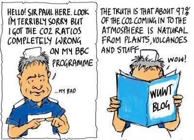
Fig.10 Cartoon by Josh on misstatements of the carbon cycle by Sir Paul Nurse,
President of the Royal Society, one of the authorities relied on by the Garnaut Updates.
Sources: various websites (Bishop Hill, Watt’s Up With That, Tamino’s Open (sic) Mind).
26You can also read