Modeling Coral Breakage at Kure Atoll - SOEST Hawaii
←
→
Page content transcription
If your browser does not render page correctly, please read the page content below
Modeling Coral Breakage at Kure
             Atoll

                 a thesis submitted to
          the global environmental science
     undergraduate division in partial fulfillment
        of the requirements for the degree of
                 bachelor of science
                          in
            global environmental science
                     August 2014

                          by
             Eric Masa Shimabukuro

                    Thesis Advisor:
             James T. Potemra, PhD.
    Hawaii Institute of geophysics and planetology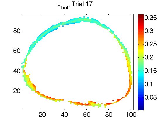
I certify that I have read this thesis and that, in my opinion, it is satisfactory in scope and quality
as a thesis for the degree of Bachelor of Science in Global Environmental Science.

                                                                               Dr. James T. Potemra
                                                       Hawaii Institute of Geophysics and Planetology

                                                  ii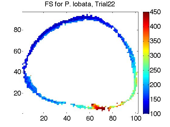
This thesis is dedicated to the hopes and dreams of my grandmother Shikako, my father
                             Norman, and my mother Laura.

                                         iii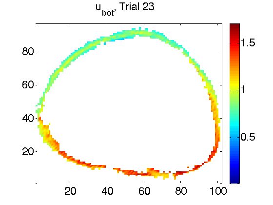
Acknowledgements

I would like to thank Dr. James Potemra, for consistent patience, guidance, editing
and motivation; Dr. Jane Schoonmaker, for editing suggestions and encouragement; my
mother Laura, for support in the darkest of times; Will McGrath for being a voice of
reason; Jennifer Killinger, for patience when I needed it most; the many members of the
Pacific Islands Benthic Habitat Mapping Center and operators of the research vessels for
gathering the bathymetry data on which all oceanographic models rely; and the many
students of the Global Environmental Science program.

                                           iv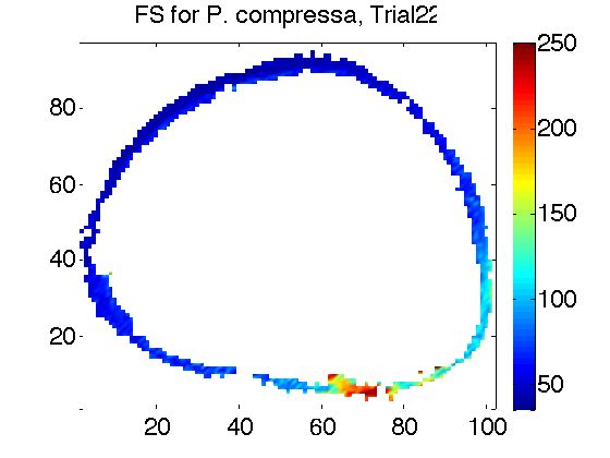
Abstract

Given the current state of climate change, coral reefs throughout the world are under

increasing pressure to survive. One factor influencing the development of coral reef

ecosystems is the energy of the surface waves passing above them. The waves cause

the water particles beneath them to flow in elliptical orbits, and the bottom of these

orbits can create strong flows which can cause coral fingers to break off. This study

follows the work of Storlazzi et al. [2005] in an attempt to model the likelihood of coral

breakage at Kure Atoll. To accomplish this, the wave field is modeled using the third

generation wave model Simulating Waves Nearshore (SWAN) [Booij et al. 1999], with

boundary conditions and wind forcing provided by WaveWatch III [Tolman 2002]. The

SWAN results for the velocity of the wave orbitals are fed into the hydrodynamic ‘Force

Balance Model’ of Storlazzi et al. [2005], which estimates the applied stress of the water

on the coral, and compares this with measured mechanical strengths. The results, which

differ from Storlazzi et al. [2005], indicate that the corals of Kure Atoll are well suited

to their environment, and are hardy enough to withstand typical wave conditions year

round. Additionally, the extreme event results indicate that corals can withstand open

ocean wave heights of up to nine meters, due in part to the fact that high resolution

modeling indicates that some of the wave energy is lost as the waves approach the shallow

coral reef zones. Finally, this study highlights the need for extensive documentation

in the presentation of mathematical models: because the documentation of Storlazzi
et al. [2005] did not explicitly define all equations utilized, it is impossible to completely

compare the results of this study and the previous one, leaving questions as to why the

results differ so greatly.

                                             vi
Contents
Dedication iii
Acknowledgements iv
Abstract v
List of Tables viii
List of Figures ix
1 Introduction 1
2 SWAN Fundamentals 3
2.1 The Action Balance Equation . . . . . . . . . . . . . . . . . . . . . . . . . . . . . . . 3
2.2 The Wave Field . . . . . . . . . . . . . . . . . . . . . . . . . . . . . . . . . . . . . . . 4
2.3 Generation by wind . . . . . . . . . . . . . . . . . . . . . . . . . . . . . . . . . . . . 5
2.4 Nonlinear Wave-Wave Interactions . . . . . . . . . . . . . . . . . . . . . . . . . . . . 8
3 Methods 11
3.1 Wind, Wave and Bathymetry Data . . . . . . . . . . . . . . . . . . . . . . . . . . . . 11
3.2 SWAN Model Setup . . . . . . . . . . . . . . . . . . . . . . . . . . . . . . . . . . . . 13
3.3 Coral Breakage . . . . . . . . . . . . . . . . . . . . . . . . . . . . . . . . . . . . . . . 16
3.4 Coral Spatial Distributions . . . . . . . . . . . . . . . . . . . . . . . . . . . . . . . . 19
4 Results 21
4.1 Boundary Conditions . . . . . . . . . . . . . . . . . . . . . . . . . . . . . . . . . . . . 21
4.2 Model Results & Coral Safety . . . . . . . . . . . . . . . . . . . . . . . . . . . . . . . 26
4.3 Extreme Events . . . . . . . . . . . . . . . . . . . . . . . . . . . . . . . . . . . . . . . 32
5 Discussion 33
5.1 What’s wrong with FSaf ety ? . . . . . . . . . . . . . . . . . . . . . . . . . . . . . . . . 33
5.2 Comparison with Coral Distributions . . . . . . . . . . . . . . . . . . . . . . . . . . . 36
6 Conclusion 38
7 References 39
viiList of Tables
1 Variables in this Document . . . . . . . . . . . . . . . . . . . . . . . . . . . . . . . . . . 4
2 Coral Measurements of Storlazzi et al. [2005] . . . . . . . . . . . . . . . . . . . . . . . . 17
3 Four Most Common Conditions from WWIII Data . . . . . . . . . . . . . . . . . . . . . 24
4 Boundary Conditions, Forcings, and Trial Types . . . . . . . . . . . . . . . . . . . . . . 26
5 Model Results, All Trials: ubot , Tp and Fsaf ety Values for the Fore-reef (10–20m) . . . . 29
6 Comparing Coral Measurements . . . . . . . . . . . . . . . . . . . . . . . . . . . . . . . 34
viiiList of Figures
1 Rayleigh Distribution of Frequency-Amplitude Spectrum . . . . . . . . . . . . . . . . . . 6
2 Comparison: Raw and Prepared Bathymetry . . . . . . . . . . . . . . . . . . . . . . . . 12
3 Daily Wind Data (WWIII) . . . . . . . . . . . . . . . . . . . . . . . . . . . . . . . . . . 22
4 Daily Wave Data: Hsig & Tp (WWIII) . . . . . . . . . . . . . . . . . . . . . . . . . . . . 23
5 Daily Wave Propogation Data (WWIII) . . . . . . . . . . . . . . . . . . . . . . . . . . . 23
6 Scatter Plot: θ vs Hsig . . . . . . . . . . . . . . . . . . . . . . . . . . . . . . . . . . . . . 25
7 Trial 1: Most Common Conditions . . . . . . . . . . . . . . . . . . . . . . . . . . . . . . 27
8 Trial 17: Southeasterly Waves . . . . . . . . . . . . . . . . . . . . . . . . . . . . . . . . . 28
9 Trials 22 & 23: Extreme Wave Height Events . . . . . . . . . . . . . . . . . . . . . . . . 30
10 Trial 22: FSaf ety Plots . . . . . . . . . . . . . . . . . . . . . . . . . . . . . . . . . . . . . 31
ix1 Introduction
Coral reefs exist in a dynamic environment and are subject to a wide range of highly variable
environmental forcings [Gove et al. 2011]. In the Hawaiian islands, corals and coralline algae compose
the physical baseline of the reefs, and are foundational to the entire ecosystem [Grigg 1998]. Because
of this, coral vigor and abundance is often a good indicator of the health of the entire reef [Jokiel
and Rodgers 2007]. Therefore, it is important to assess the factors influencing coral health, both to
establish baselines for comparative studies and to understand proper management practices [Kenyon
et al. 2008].
When considering the factors that influence corals, one cannot fully describe the environment
without an inclusion of the constant movement of the medium in which corals grow—i.e. the wave
motions of the reef zone. To that end, there have been a collection of studies that examined the
qualitative relationship between wave energy and coral distributions [Grigg 1998, e.g.], however wave
energy in these studies is often overly simplified [Storlazzi et al. 2005]. Additionally, whilst surface
wave data (such as significant wave height and period) are certainly correlated with the effects of
waves on coral [Storlazzi et al. 2005][, this study], the energy surface phenomena are translated
to corals through a complex suite of fluid dynamics [Komar 1998, e.g.] that necessitate a deeper
analysis. Computer models, in this case Simulating Waves Nearshore (SWAN) [Booij et al. 1999],
are well suited for this task because they are by definition composed of such physical equations.
Third generation wave models such as SWAN and WaveWatch III [Tolman 2009] use the spectral
action balance equation to track the frequency and direction of waves. Through a combination of
statistical wave observations and the two aforementioned variables, all relevant information about
waves on the sea can be determined [Holthuijsen 2007]. In the relatively shallow coastal zones where
corals exist, additional wave physics (which are not relevant in deep, pelagic waters) come into play,
1and it was for this reason that SWAN was developed. This makes SWAN perfectly suited to the
modeling of wave physics to be applied to coral communities, where small time and spatial scales
can create significant changes in the wave field [Holthuijsen 2007]. It is hoped that by running
SWAN with high resolution bathymetry and processing the output through the hydrodynamic coral
breakage model of Storlazzi et al. [2005], the influence of wave energy on coral populations in the
Hawaiian atolls can be better quantified.
For this study, Kure Atoll was selected as a case-study because it had easily available, very high
resolution bathymetry, and because it had the greatest climatological range of wave energy [Gove
et al. 2011] which should allow for a better assessment of variability in wave conditions. Kure Atoll is
located at the northern tip of the Papahanaumokuakea Marine National Monument, more commonly
known as the Northwestern Hawaiian Islands (NWHI). Centered at 28◦ 25’N, 178◦ 20’W, Kure is not
only the northernmost atoll of the NWHI, but also the northernmost tropical reef atoll in the world
[Dana 1971]. While Kure’s remote location has spared the atoll’s barrier reef from many of the
direct effects of anthropogenic activities, Kure bears several reminders of humanity’s global reach.
Green Island, which is about 86.67 hectares (ha) in area and is located on the southwest corner of
Kure, is the only appreciable land mass within the atoll. Green Island supports two permanent
man-made structures, a runway and U.S. Coast Guard station, both of which are abandoned and
unmaintained [PIBHMC 2011]. As the northernmost atoll in the NWHI, Kure’s proximity to the
North Pacific Current (the northern component of the North Pacific Gyre) has lead to Kure being
speckled with floating debris [Boland et al. 2006]. In addition to these localized anthropogenic
influences, global warming has contributed to at least two occurrences of coral bleaching in the past
fifteen years [GS et al. 2003; JC and Brainard 2006], an alarming occurrence considering that Kure
is the northernmost tropical coral reef ecosystem.
22 SWAN Fundamentals
2.1 The Action Balance Equation
SWAN is similar to WaveWatch III [Tolman 2009] in that both models solve the (spectral) action
balance equation (presented in the style of Holthuijsen [2007] Eq. 9.3.1):
∂N (σ, θ; x, y, t) ∂cg,x N (σ, θ; x, y, t) ∂cg,y N (σ, θ; x, y, t)
+ + +
∂t ∂x ∂y
∂cθ N (σ, θ; x, y, t) ∂cσ N (σ, θ; x, y, t) S(σ, θ; x, y, t)
+ = (1)
∂θ ∂σ σ
where N is action density, σ is the relative frequency, θ is the propagation direction (normal to
the wave crest), x and y are horizontal cartesian coordinates, t is time, and S is the source term,
representing the cumulative effects of energy sources and sinks. The semi-colon in N (σ, θ; x, y, t)
denotes the fact that action density is a direct function of σ and θ (due to spectral energy balance,
see below). Briefly describing the left-hand side of the equation: the first term represents the local
(i.e. at that grid point) rate of change in N with time, the second and third terms describe the
propagation of N in horizontal space (cg,x and cg,y are the group velocities in the x and y directions,
respectively), the fourth term accounts for changes in wave direction with cθ as the rate of change of
direction with time (dθ/dt), and the fifth term represents changes in wave frequency (i.e. period, T ).
For quick reference, Table 1 contains a brief description of all mathematical symbols used in this
document. The rest of this chapter will be dedicated to describing the mathematical and statistical
basis for the action balance equation as it is incorporated in SWAN.
3Table 1: Variables in this document
Variable
Symbol Description Unit Source
Underbar η Random variable — ‡ 33
N Action Density m2 /Hz/rad ‡ 38
ω Radian Frequency rad/sec ‡ 123
σ Relative Frequency rad/sec ‡ 218
θ Wave Propagation Direction rad ‡ 43
cg Group Velocity m/s ‡ 127
S Generic Action Balance Source/Sink m2 /Hz ‡ 173
H Wave Height m ‡ 27
T Wave Period s ‡
L Wave Length m ‡
η Sea Surface Elevation m ‡ 31
α Phase (of Harmonic Wave) rad ‡ 31
f Frequency (1/T ) Hz ‡ 31
αwind Initial Linear Wave Growth Term ?? ‡ 290
βwind Non-linear Wave Growth Parameter ?? ‡ 290
Sin,wind Source Term, Wind Input m2 /Hz ‡ 290
θwind Wind Direction rad ‡ 290
u∗ Friction Velocity (of wind) ?? ‡ 290
G Low Frequency Growth Cut-Off ?? ‡ 290
γM iles Miles Parameter for Wave Growth ?? ‡ 291
κ von Kármán Constant ND ‡ 291
λcrit Critical Wave Height ND 3 1634
Snl4 Source term, quadruplets m2 /Hz/s ‡ 186
• † Booij et al. [1999]
• ‡ Holthuijsen [2007]
• 3 Janssen [1991]
2.2 The Wave Field
From linear wave theory, the height of waves on the sea surface (η) can be described by the random-
phase/amplitude model [Holthuijsen 2007, p.44]. In the idealized, two-dimensional case, varying in
time, η would be the sum of a large number of harmonic waves. Each wave would have an evenly
distributed (0 < α ≤ 2π) random phase, α and a Rayleigh distributed amplitude, a. Therefore,
4at any point and time (x, y, t), η (which is a random1 variable, denoted by the underline: η) is
described by (Eq 3.5.20 of) Holthuijsen [2007]:
max jX
iX max
η(x, y, t) = ai,j cos(2πfj t − ki xcos(θj ) − ki ysin(θj ) + αi.j ) (2)
i=1 j=1
where ki is the wave number (2π/L) of an individual harmonic wave that is traveling in the direction
θj with a frequency of fi .
To solve Eq. 2, the range of possible frequencies of ocean waves (0.01–1.0 Hz in open seas
[Holthuijsen 2007, p. 34]) is discretized to jmax number of frequency bins (fj ). Each frequency bin
will correspond to a statistically likely amplitude, a, and collectively, the expected amplitudes (as a
function of frequency) follow a Rayleigh distribution with a high frequency tail (Fig 1).
2.3 Generation by wind
At sea, waves are generated by turbulence at the interface between two fluids: the air above and the
water below. From a modeling standpoint, the transfer of wind energy to ocean waves is a source
term (Sin,wind ) divided into an initial linear growth term (αwind ), and a more prominent non-linear
growth term, which is the product of the current energy density E and a nonlinear parameter βwind .
Sin,wind (σ, θ) = αwind + βwind E(σ, θ) (3)
The linear component of this formulation has been incorporated as a means of empirically generating
waves on a smooth ocean surface, and is accredited to Cavaleri and Malanotte-Rizzoli [1981] with a
low frequency cut-off modification added by Tolman [1992]:
−3
1.5×10 [u∗ cos(θ − θwind )]4 G for |θ − θwind | ≤ 90◦
g 2 2π
αwind = (4)
0 for |θ − θwind | > 90◦
1
In this case, random implies that the variable could not be predicted exactly
5Figure 1: Example Rayleigh distribution of wave amplitude as a function of
frequency [Holthuijsen 2007, p.35].
where u∗ is the friction velocity of the wind vector (to be discussed below), and G is the Tolman
[1992] cut-off function:
−4 ]
G = e[−(28σu∗ /0.26πg) (5)
The addition of G is necessary because initial wave growth takes place at high frequencies [Tolman
1992, p.1097], with energy transferred to lower frequencies as the sea state develops [Holthuijsen
2007]. Without the cutoff, energy would be erroneously added to low-frequency waves causing
unrealistic spectral distributions.
While initial generation can be an important aspect of idealized test cases, most real-world
scenarios will not begin with the sea completely at rest, and the wave field will already be populated
by waves from areas anon. In this case, with waves already present, the transfer of energy from the
6wind to the waves becomes a function of surface pressure at the wind-wave interface. According to
Miles [1957], waves distort the flow of the wind above them, causing otherwise horizontal streamlines
to follow a profile similar to the sea surface. This in turn causes the wind to exert a greater surface
pressure on the windward side of the wave, pushing water particles downward, and a reduced
surface pressure on the leeward side, pulling water particles upward [Holthuijsen 2007, p. 179]. The
alternating push and pull of the surface pressure transfers additional energy to the wave, causing it
to grow in height. Finally, as the wave height increases, the wave can interact with a larger vertical
section of the wind, increasing effectiveness of the growth mechanism and creating a non-linear
positive-feedback mechanism [Miles 1957].
The Miles feedback mechanism is the primary means of energy transfer from wind to ocean
waves. In SWAN, this feedback is accounted for in the second term of Eq 3, where the inclusion of
E(σ, θ) (which is the energy density, as derived from the amplitude spectrum, see Fig 1) provides
for the dependence on wave height. The parameter βwind is calculated following WAM Cycle IV
[Komen et al. 1994]:
ρair u∗ 2 2
β = max 0, γM iles cos (θ − θwind σ (6)
ρwater c
wherein the Miles parameter (γM iles ) has been retuned by Janssen [1991] to better match observations,
yielding:
1.2
γM iles = λcrit ln4 λcrit (7)
κ2
with the von Kármán constant κ = 0.41, and the dimensionless ‘critical height’ (λcrit ) given by
[Holthuijsen 2007, p. 291]:
gze
λcrit = exp[κc/|u∗ cos(θ − θwind )|] for λcrit ≤ 1 (8)
c2
7and
βwind = 0 for λcrit > 1 (9)
In SWAN, equations 6–9 are solved using the relationships established by Janssen [1991].
Procedurally, the iterative approach of Mastenbroek et al. [1993] is used. First, the wave stress
(τwave ), which represents the effect of the waves on the wind, is solved for:
Z 2π Z inf
τwave = ρwater σβE(σ, θ)dθdσ (10)
0 0
using E(σ, θ) from the previous time step. Next, the friction velocity (u∗ ), surface roughness length
(z0 ), effective surface roughness length (ze ), and total shear stress (τ = τt + τw , with τt representing
turbulence) are found by iterating the following three equations:
u∗ 10 + ze + z0
U10 = ln (11)
κ ze
u∗
z0 = 0.01 (12)
g
z0
ze = p (13)
1 − τwave /τ
where U10 is the user input wind at 10m elevation, τ is related to u∗ via τ = ρair u2∗ , and Eq 12 is a
Charnock-like relation with a constant of 0.01 [SWAN Team 2013a, p. 19].
2.4 Nonlinear Wave-Wave Interactions
Nonlinear wave-wave interactions are a type of resonance interaction, and are the primary mechanism
of energy transfer between waves. There are two distinct types of nonlinear wave-wave interactions,
triads and quadruplets, which describe interactions between 2–3 and 4–5 wave groups, respectively
[Holthuijsen 2007]. In the case of triad wave-wave interactions, two wave groups of frequencies f1
and f2 , traveling toward each other at directions ~k1 and ~k2 will cross. The diamond pattern formed
8by the waves and troughs of the crossing groups will form a new wave group with a frequency that
satisfies f1 + f2 = f3 and a direction that satisfies ~k1 + ~k2 = ~k3 . Triad wave-wave energy transfers
can also occur if a third wave group with frequency f3 and direction ~k3 crosses the diamond pattern
formed by wave groups 1 and 2. This phenomena is well illustrated by Figure 6.19 of Holthuijsen
[2007]. In either case, the total energy in the system remains constant, and is simply redistributed
between the three resulting wave groups.
The primary limitation on triads is that these interactions can only occur in very shallow water,
where waves are said to be non-dispersive, and the phase speed (cshallow ) is a function of gravity (g)
√
and depth (d) alone, i.e. cshallow = gd. In SWAN, triads can only occur in water shallow enough
to meet the previous condition, or in areas where the water is shallow enough for near resonance to
occur, in which case energy transfer and phase-coupling affect all three resulting wave components
[Holthuijsen 2007, p. 271]. As this paper focuses on wave energy, it is also important to consider
how this quantity is handled. The energy transfer between the triad waves depends on the relative
magnitudes of the three phases: φ1 , φ2 , and φ1 + φ2 = φ3 , which are used to compute the biphase
(β1,2 ):
β1,2 = φ1 + φ2 − φ3 (14)
á la Holthuijsen [2007, p. 289]. In very shallow water, waves become saw-toothed and the biphase
approaches −90◦ , which leads to the operational equation
π π δU r
β1,2 = − + tanh (15)
2 2 Ur
[SWAN Team 2013a, p.30], where Ur is the Ursell number, representing the ratio of steepness to
relative depth, and δU r is a coefficient that varies within the range of 0.2–0.6 [Holthuijsen 2007,
9p.274], and is by default set to 0.2 [SWAN Team 2013a, p.30].
steepness 2
g Hs Tm01
Ur = = √ (16)
relative depth 8 2π 2 d2
with Hs as the significant wave height, and Tm01 as the ratio of the zeroth and first moment of the
variance density spectrum ( m
m02 ). Because the Ursell number represents the degree of nonlinearity
01
of the wave, and because triads are inherently nonlinear, Ur determines whether or not triads take
place, and they are only accounted for when 0 ≤ Ur ≤ 1 [SWAN Team 2013a, p.30].
To speed up computation time, SWAN uses the ‘Lumped Triad Approximation’ (LTA) of
Eldeberky [1996].
Quadruplets, the second type of wave-wave interaction, can occur in both shallow and deep
water, and are largely responsible for wave-wave energy transfer in the latter. Quadruplets form via
resonance, in a similar fashion to triads. In this case of quadruplets, instead of two wave components
meeting, two pairs of wave components must meet, the first pair with frequencies and directions f1 ,
f2 , ~k1 and ~k2 , and the second pair with frequencies and directions f3 , f4 , ~k3 and ~k4 . When the both
pairs cross at the same location (i.e. the diamond patterns are superimposed), f1 + f2 = f3 + f4 ,
and ~k1 + ~k2 = ~k3 + ~k4 , resonance, and therefore energy transfer, occurs [Holthuijsen 2007, p. 184].
The source term for quadruplet interactions (Snl4 ) is computed with the Boltzmann integral of
Hasselmann [1962], reformatted in terms of energy density by Holthuijsen [2007]:
Z Z Z Z
Snl4 (~k4 ) = T1 (~k1 , ~k2 , ~k3 )E(~k1 )E(~k2 )E(~k3 )d~k1 d~k2
Z Z Z Z
− E(~k4 ) T2 (~k1 , ~k2 , k~4 )E(~k1 )E(~k2 )d~k1 dk~2 (17)
where E(f, θ) has been recast in terms of ~k, while T1 and T2 are transfer coefficients comprised of
the variables ~k, ω, and H of the waves involved [Hasselmann 1962, p.497].
103 Methods
3.1 Wind, Wave and Bathymetry Data
The Kure Atoll bathymetry data in this study were gathered by NOAA and the Pacific Islands
Benthic Habitat Mapping Center (PIBHMC) in 2006, and are available from http://www.soest.
hawaii.edu/pibhmc. The in situ data were gathered using a 30 kHz Simrad EM300 sonar and a
300 kHz SImraid EM3002d sonar aboard the NOAA R/V Hilialakai, and a 240 kHz RESON 8101-ER
sonar aboard the NOAA R/V AHI (Acoustic Habitat Investigator) [NOAA 2007]. Sonar data
were supplemented by IKONOS satellite imagery from the NOAA/NOS/NCCOS/CCMA2 Remote
Sensing Team, with IKONOS providing all of the data from 0–16 m depths. The final gridded
bathymetry was created by dividing the satellite and sonar data into identical grids, and averaging
the values where the datasets did not match. According to the authors, the depth data are accurate
to within ±1 m.
To prepare the bathymetry data for SWAN, the GMT (‘.grd’) files were loaded into MATLAB,
and missing values were filled in with an average of their closest neighbors. All grid cells surrounding
the known Kure bathymetry were set to a constant depth of 1000 m. While this is not realistic, it
is unlikely that this simplification will have an impact on surface wind waves [Holthuijsen 2007].
As can be noticed in the Fig 2, the iterative procedure used to fill in the missing values caused
‘ridges’ to appear on the north, southeast, and southwest corners of the island. The shallowest of
these artifacts is around 700m depth, and at this depth it is still unlikely that surface waves will be
affected. The resulting bathymetry grid was defined from a depth of 1000m at the edges, to 0m at
the barrier reef encircling the island, the only missing values (which will be interpreted as land in
2
NOS: National Ocean Service, NCCOS: National Center for Coastal Ocean Science, CCMA: Center for Coastal
Monitoring and Assessment
11(a) Raw bathymetry data from PIBHMC. (b) Bathymetry data that were fed into SWAN for
modeling simulations.
Figure 2: Visual comparison of the raw bathymetry data (a) and the bathymetry
data used by SWAN (b) which has had all missing values filled. Green Island is
left as missing data points, which SWAN interprets as land.
SWAN) were the cells defining Green island. This grid was then saved as an ascii file to be read by
SWAN.
The wind and boundary wave data are provided by WaveWatch III [Tolman 2002] version
2.22, and are freely available at http://polar.ncep.noaa.gov/waves/download.shtml?.
Hindcast data at a global spatial resolution of 0.5◦ are available from February, 2005 to December,
2013, with a temporal resolution of 3 hours. For the present study, hindcast data are especially
useful because the data and model are adjusted to best match observations, providing more realistic
statistics. To estimate the recent trends in wind and wave activity around Kure, MATLAB was used
to extract wind and wave data from the WWIII dataset at the nearest grid point, located at 178◦ 30’
W, 28◦ 30’ N. A daily mean was attained by averaging (less the missing values) the 3-hour intervals.
Wave data provided were significant wave height (Hsig ), propagation direction (θ), and peak
period (Tp ). Wind data were available as Uwind and Vwind horizontal vector components. To facilitate
12the sorting of these data, the direction (in SWAN convention, measured in degrees counter-clockwise
(CCW) from the positive x axis) was computed using the arctangent function and the sign of the
vectors (to determine the quadrant):
arctan(Vwind /Uwind ) if U ¿ 0 and V ¿ 0
θwind = arctan(V ◦ (18)
wind /Uwind + 180 if U ¡ 0 and V ¿ 0 or U ¡0 and V ¡ 0
arctan(Vwind /Uwind + 360◦ if U ¿ 0 and V ¡ 0
The magnitude of the wind vector was computed using the Pythagorean theorem. Data were sorted
into discrete bins containing a range of values. Wind and wave propagation directions were sorted
into 10◦ bins ranging in total from 0◦ to 360◦ . Significant wave height was sorted into 1m interval
bins (i.e. 0 ≤ Hsig < 1, 1 ≤ Hsig < 2 . . . Hsig ≥ 10), with the final bin containing all occurrences
of significant wave heights greater than (or equal to) ten. Wind magnitudes were similarly sorted,
with the exception that the range covered 0–20 m/s. Wave periods were sorted into two second
interval bins ranging from 0 to 18 s. From the bin data, the top four ranges for each parameter
were determined, and run in various combinations to assess both the influence of the individual
components as well as the long term average wave energy. Additionally, three ‘extreme’ event
scenarios were run in order to assess the upper climatological limits of expected wave energy. The
input parameters were, in this case, found by manually selecting the two largest wave events in the
two most common directional octants: NW (3̃00◦ ) and SE (1̃00◦ )
3.2 SWAN Model Setup
The SWAN computational grid covered the entire area of the original Kure atoll bathymetry, divided
into 100m×100m cells numbering 280 in the x direction and 373 in the y direction. In the wave
13spectral space, the frequency range used was flow =0.01 to fhigh =1.0. These data were discretized
into 49 spectral bins according to the following equation [SWAN Team 2013b]:
log(flow /fhigh
number of bins = (19)
log(1 + ∆f /f )
in order to comply with the relationship of ∆f /f = 0.1, which is required for the DIA quadruplet
approximation. Directional space encompassed 360◦ , and was discretized into 2◦ increments (180
bins total). Uniformly distributed wind forcing was applied as a constant across the entire grid, with
the magnitude and direction determined by the aforementioned sorting procedure. Wave forcing
was fed from two of the four grid sides, as determined by direction of propagation. For example,
waves of θ = 120◦ (traveling NW) would enter from the south and east borders. For each scenario,
a ‘stationary’ computation was done, largely in order to reduce the overhead associated with a
time-stepping process. In essence, a stationary computation solves Eq 1 with the first term equal to
zero (∂N (σ, θ; x, y, t)/∂t = 0).
SWAN allows the user to adjust many parameters in order to accommodate a wide range of
uses, some of these options were tailored for this study, as will be discussed below. The user-defined
baseline whence the depth is measured was set to the height of the highest fringing reefs of the
bathymetry file (0.0m), representing the water level of a completely flat sea surface. The minimum
depth, above which waves are forced to break, was set to 0.05m. The wind information fed to SWAN
is assumed to be the wind velocity at 10m elevation (U10 ), and these data are converted to the
friction velocity u∗ using the wind-drag coefficient CD [SWAN Team 2013a] via the relationship:
u∗ = U10 CD (20)
In order to prevent overestimation of CD under high wind conditions [Zijlema et al. 2012], a cap of
2.5×10⁻³ is suggested by the SWAN team, and has been implemented for this study. Boundary
14waves were fitted to the JONSWAP spectrum, with a (default) peak enhancement parameter of
γpeak = 3.3. As dictated by the WWIII data, the input period was the peak period Tpeak (as opposed
to the other commonly used period, the mean period Tm01 ). Because the WWIII wave directions
were so irregular (see next chapter), a high degree of directional distribution (37.5◦ ) was given for the
incoming wave data, in the hopes that this would better approximate the random nature of surface
waves. In SWAN, bottom friction accounts for some energy dissipation and is an important aspect of
modeling wave energy. The JONSWAP formulations of Hasselmann et al. [1973] are used to account
for friction, where the friction coefficient (Cf ric ) is a constant 0.038 m2 /s3 . The value was picked
because swell is the dominant form of energy input into the grid, and SWAN Team [2013b] suggested
this value for those conditions. As a note however, the choice of Cf ric = 0.038 conflicts with the
SWAN model practice of using a higher Cf dic value (0.067 m2 /s3 ) for directional distributions above
30◦ . Despite the rather coarse model resolutions, the attempt was made to include triad interactions
(using the LTA method) with the standard SWAN parameter values. Diffraction, however, was
disabled, largely because the SWAN authors suggested that a resolution of 10–20% of the dominant
wavelength be used for any diffracting obstacle, an impossibility at the 100m resolution of the
current model. The parameter that controls the centrality of the refraction scheme (with 0 being
fully central, and 1 being a first order upwind scheme) was left at the default value of 0.5; this
option provides a balance between the accuracy and instability of a fully central scheme, and the
stability and diffusivity of a fully upwind scheme. Finally, the turning rates in spectral space cθ and
cσ (with σ as the relative frequency) are both limited to the upper Courant-Friedrichs-Lewy (CFL)
value of 0.5, as suggested by SWAN Team [2013b].
153.3 Coral Breakage
Probability of coral breaking was estimated using the methodology of Storlazzi et al. [2005] and
Massel [2013]. In this manner, a coral head is assumed to be an idealized cylinder, with height hcor ,
radius rcor , and basal radius rcbase (see Table 6). The total pressure applied to the coral is a sum of
four forces: lift Fcl , drag Fcd , weight Fcg and the internal force, Fci . The lifting force is caused by
the acceleration of water as it flows over the coal head, and is calculated as [Storlazzi et al. 2005,
Eq 3]:
1
Fcl = ρClif t u2bot 2rcor hcor βhide (21)
2
where Clif t = 15 is the lift coefficient for a cylindrical shape [Hoerner 1965], and βhide is a hiding
parameter that allows the user to fine-tune the density of coral cover, with βhide = 0 being completely
hidden by other corals and βhide = 1 being completely exposed. Following Storlazzi et al. [2005],
βhide is set to 0.9, however the authors of that paper state that this choice is somewhat arbitrary.
Note that where Storlazzi et al. [2005] uses the average of several near-bed wave orbital velocities in
their formulations (ū in their notation), this study uses the maximum bottom wave orbital velocity,
ubot as is output by SWAN. The drag force acting on the coral is simply:
1
Fcd = ρCcdrag u2bot 2rcor hcor β (22)
2
with Ccdrag = 0.85, chosen by Storlazzi et al. [2005] due to measurements by Denny [1988] and
Denny [1993] and Gerhart et al. [1993]. The gravitational force (i.e. the relative weight of the coral
2 h
in seawater) is a function of volume (πrcor cor ) and the relative density:
2
Fcg = (ρcor − ρ) gπrcor hcor (23)
16Table 2: Replication of Table 1 in Storlazzi et al. [2005], displaying coral morpho-
logical data and mechanical strengths. Coral measurements were gathered by
Storlazzi et al. [2005], and mechanical strengths are from Rodgers et al. [2002].
Coral Species hcor (m) rcor (m) rcbase (m) σresisti (MPa)
Montipora capitata 0.20 0.10 0.06 3.5
Porites compressa 0.15 0.02 0.02 5.3
Porites lobata 1.00 0.50 0.45 6.2
Pocillapora meandrina 0.20 0.13 0.07 7.0
where ρcor = 1450kg/m3 is the coral skeletal density [Lough and Barnes 1992]. The final force
considered, the inertial force, is due to the oscillatory flow of the passing wave causing acceleration
and deceleration of the fluid around the coral head. The inertial force is computed via
51 2
Fci = ρπrcor hcor af luid (24)
24
where af luid is reported by Storlazzi et al. [2005] as being “a function of ubot and T ”, but is not
otherwise absolutely defined.
To seek out the equation for af luid , the source of the formulations used by Storlazzi et al. [2005],
(i.e. Massel [2013]) was consulted. Massel [2013] reports the inertial force as being the summation
of two components (Fci = Fci1 + Fci2 ), the first being the product of the coral mass and af luid :
Fci1 = ρVcor af luid (25)
and the second being due to the mass of the coral. This second component is derived from the
formulation by Milne-Thompson [1960] for kinetic energy (KEs ) acting on a sphere3 :
3 3 !
3 D2ex
pi Dex
KEs = ρ 1+ u2bot (26)
3 2 16 hex
Dex
where Dex and hex = 2 are coral diameter and height from sea floor, respectively, and the subscript
‘ex’ denotes that these are merely included to complete the example. Following Kochin et al. [1963],
3
The shape considered in Eq 26 is irrelevant because the equation is only included to illustrate the derivation of
af luid used in this study.
17the kinetic energy is converted to the second force component by taking the partial derivatives, first
with respect to ubot :
∂KEs 19 3
= πρrcor ubot (27)
∂ubot 24
and then with respect to time (t):
∂ 2 KEs 19 3
= πρrcor af luid (28)
∂ubot ∂t 24
D
where 2 has been replaced with rcor . The key piece of information from Eqs 26–28 is that af luid is
found by taking the derivative of ubot with respect to time, implying that af luid is simply:
ubot
af luid = (29)
T /2
where the period (T ) is halved because the acceleration only occurs for the first half of the waves
passing. Another difference between this study and Storlazzi et al. [2005] is that the authors used
the peak period T = Tp , and this study uses the mean period T = Tm01 .
The horizontal forces Fci and Fcd act above the coral base and create an overturning moment
about the neutral axis of the coral, lifting the upstream edge and forcing down on the downstream
edge [Massel 2013]. The duality of this creates tension on the upstream edge and compression on the
downstream edge, and will cause the coral to fail if either stress is greater than the corresponding
(tensile or compressional, respectively) mechanical strength of the coral. Thus, the stress on the
coral structure per unit area (σapplied ) is the greater of:
1
Fcg + Fcl 2 (Fci + Fcd )2rcor rcbase
σapplied = 2 ± 1 4
(30)
πrcbase 4 πrcbase
wherein the denominator of the second term on the RHS is the second order moment of the basal
area [Massel 2013]. The combination of forces Fcg and Fcl in the first term on the right-hand side
(RHS) of Eq 30 is due to the fact that these two forces act in the vertical plane, whereas Fci and
Fcd act in the horizontal, as previously mentioned.
18Corals are brittle and fail with negligible deformation, negating the need for considerations where
the coral bends but does not break [Storlazzi et al. 2005]. Again following Storlazzi et al. [2005],
once the larger σapplied value has been taken from Eq 30, it is compared with the species-specific
resistive force per unit area (σresist ) to create a ‘Factor of Safety’ (Fsaf ety ):
σresist
Fsaf ety = (31)
σapplied
The values for σresist were calculated by Rodgers et al. [2002], and can be found herein in Table 6.
Using this simple metric, corals will be very likely to break when Fsaf ety ≤ 1, because at that point
the applied stress is greater than the mechanical strength of the coral.
3.4 Coral Spatial Distributions
It is quite fortunate that the main Hawaiian Islands and their distant ancestor Kure share many
of the same corals, because this allowed the morphological coral data of Storlazzi et al. [2005] to
be used to estimate coral breakage at Kure Atoll. Coral species distributions were provided by
Kenyon et al. [2008], who in 2000, 2002 and 2003 conducted coral cover surveys using a combination
of video-recorded transects, experienced towed divers, and still photoquadrats. The coral data of
Kenyon et al. [2008] are available only for depths above 20m, however, ubot decreases very quickly
with depth, and the the upper 20m are the depths most likely to be afflicted by wave-induced coral
breaking [Storlazzi et al. 2005]. The towed-diver surveys of Kenyon et al. [2008] were spatially
separated around the fore- and back-reef of the atoll, and were therefore quite suited for use in this
study. Additionally, towed-diver surveys are reported by the author to be more reliable than the
other methods, due to the fact that divers are able to survey a much wider area.
To compare the Fsaf ety values from the coral breakage model with the coral spatial information,
the grid files for ubot and Tm01 that were output by SWAN were first loaded into MATLAB. Then,
19Eq 21–24, 30 and 31 were applied (in that order) for each cell across the grid. Next, Fsaf ety values
for grid cells corresponding to depth ranges reported by Kenyon et al. [2008] were analyzed for three
areas: the fore-reef (depths: 10–20m), the back-reef (depths: 0–5m4 ), and the lagoon, which was
only analyzed in one area which corresponds to the study site in Fig. 2 of Kenyon et al. [2008]. All
grid cells of Fsaf ety that did not correspond to a depth of the appropriate range were removed (set
to NaN) and the resulting matrices were visually analyzed using colored plots to determine ranges
and spatial variability of Fsaf ety .
4
While Kenyon et al. [2008] reports only examining depths of 0.7–1.4m in their study, this range was expanded to
include more grid points in the model data.
204 Results
4.1 Boundary Conditions
WaveWatch III data were available from February 2005 to December 2013, and time-series and
sorted bins (as per the process described in Chapter 3.1) are displayed in Figs. 3–5. Wind direction
(θwind ) time-series data (first plot, Fig 3) ranged from 10–350◦ , and featured greater variability in
the northern hemisphere winters. Statistically, the θwind data featured a mean of 1̃70◦ , and the top
four 10◦ bins were: 190–200◦ , 180–190◦ , 200–210◦ and 170–180◦ in that order (second plot, Fig 3,
Table 3). The hourly θwind data were available in three hour intervals, and were used to compute
a daily average of eight values. The daily standard deviation of this averaging process ranged
from 0̃–188◦ , with an average of 36◦ and 62% of calculated deviations were below 20◦ . Additionally,
standard deviations for θwind were often greater during periods of greater wind variability.
Wind magnitudes ranged from 1–20 m/s (rounded to closest integer), with an average of 6.9 m/s.
The wind magnitude data highlighted a consistent trend of greater magnitudes during the Kure
winter, with strongest annual winds always appearing during winter months, with one exception in
2012. (third plot, Fig 3). After sorting into 1 m/s bins, the top four wind magnitude bins were: 5–6,
6–7, 7–8 and 8–9 m/s, in that order (fourth plot, Fig 3, Table 3). The daily standard deviations
values for wind magnitude data ranged from 0̃ to 6̃ m/s, with an average of 1.2 m/s, and with 75%
of all values below 1.5 m/s (64% of values between 0.5 and 1.5). And finally, showing a similar
temporal pattern to wind direction, the standard deviation values for wind magnitude were greater
during periods of stronger wind activity (i.e. Kure winters).
21Figure 3: Daily wind data at 178.5◦ W,28.5◦ N., averaged from 3-hourly output
from WWIII. Top plot is wind direction in degrees CCW from due east. Second
plot is the daily data from the top plot sorted into 10◦ directional bins ranging
from 0–360◦ . The third plot is a time series of wind magnitude in m/s. The
fourth plot is the wind magnitude data from the third plot, sorted into 1m bins.
Significant wave heights displayed a strong seasonal signal, rising in the fall and peaking in early
winter (first plot, Fig 4). Wave heights ranged from 0.7–9.25 m, with an average of 2.6 m. The top
significant wave height bin, 0–1 m, contained 36.85% of all values, the next three largest bins were:
2–3 m, 3–4 m and 4–5 m (second plot, Fig 4, Table 3). Standard deviations for the significant wave
height were highest during the periods of high wave activity (i.e. fall/winter) and ranged from 0 to
2 m, with 94.8% of values between 0 and 0.32 m.
Peak period (Tp ) ranged from 4 to 17.6 s, with a mean of 10.2 s. Peak period also tracked
temporally with significant wave height, rising above 10 s in the winters and dipping below 10 s in
the summers (third plot, Fig 4). Standard deviations for daily Tp averages showed a fairly noisy
5
This value was used for an ’extreme event’ analysis
22Figure 4: Daily wave Hsig Tpeak data at 178.5◦ W,28.5◦ N., averaged from 3-
hourly output from WWIII. The top plot shows Hsig in m. The second plot
displays the Hsig data from the top plot, sorted into 1m bins. The third plot
shows Tpeak in seconds. The fourth plot shows the data from the third plot,
separated into 2s bins.
Figure 5: Daily wave propagation direction data at 178.5◦ W,28.5◦ N., averaged
from 3-hourly output from WWIII. The top plot shows the direction of wave
propagation (θ) measured CCW from due east. The second plot shows the data
from the top plot, sorted into 10◦ bins.
23Table 3: Four most common conditions for wind and wave forcing data from
WWIII, as dictated by the sorting displayed in Figs 3–5
Rank Waves Winds
Hsig Tm01 θ Mag. θwind
1 1–2 8–10 300–310 5–6 190–200
2 2–3 10–12 310–320 6–7 180–190
3 3–4 12–14 100–110 7–8 200–210
4 4–5 6–8 290–300 8–9 170–180
time-series with peaks throughout the year. The standard deviations ranged from 0–5.6 s with an
average of 0.64 s, and 90.7% of data points below 1.6 s. Sorting into 2 s bins showed that 42.7% of
Tp values fell within the range of 8 to 10 s (the largest bin), with bins for 10–12 s, 12–14 s, and 6–8
s ranking second, third, and fourth, respectively.
Wave directions (θ) spanned nearly the entire directional space (3–358◦ ) as measured CCW
from due East (the positive x axis). Time-series data showed wave directions without a strong
seasonal signal, however there was a tendency toward northwesterly waves (300–330◦ ) during the
northern hemisphere fall (first plot, Fig 5). Standard deviations for wave direction ranged from
0–189◦ with 63% of values below 10.5◦ (the mean was 30◦ ). Temporal evaluation of the standard
deviation revealed that the signal was consistently noisy, often spiking between 0 and 100◦ +. Sorting
into 10◦ bins showed a dual-peaked distribution, with the larger peak (27.8% of data points) between
290 and 320◦ , and the smaller peak (16.7% of data points) between 90 and 120◦ (second plot, Fig 5).
The top four bins for wave direction were: 300–310◦ , 310–320◦ , 100–110◦ and 290–300◦ (Table 3).
The four largest bins for each boundary variable were used to simulate the statistically likely
wave conditions around Kure Atoll, as well as to assess the influence of each parameter on Fsaf ety .
In general, the strategy with model trials was to set all parameters equal to the values of the top
ranked bins (i.e. the ‘Most Common Conditions’, or MCC) and then to vary one boundary condition
24Figure 6: Scatter plot of θ vs Hsig , as derived from the daily WWIII data.
through the four possible values (Table 4). Once it was seen that significant wave height had the
greatest influence on Fsaf ety , all four Hsig values were evaluated for conditions with southeasterly
swell (100–110◦ ). In addition to the statistically likely bin data used to simulate the most common
conditions, three extreme events were analyzed to determine the potential threat to Kure’s coral
communities. Two of the extreme events selected were significant wave height based, one trial for
each of the primary wave directional sectors (3̃00◦ and 1̃00◦ ). The two trials featured the highest Hsig
in each sector: 9.2 m approaching from the northwest, and 7.5 m approaching from south-southeast
(Fig 6). The third trial was selected based on peak period, for which the highest daily Tp value
(17.6 s) was selected. For extreme conditions, all other boundary data were taken from the day
corresponding to the selected values, (as opposed to using the statistically likely data) and all
boundary data can be found in Table 4.
25Table 4: Boundary Conditions, Forcings, and Trial Types
Trial Info Waves Wind
Trial Flag Hsig Tp θ Mag. θwind
1 1.5 9 305 5.5 195
2 1.5 9 305 8.5 195
3 1.5 9 295 5.5 195
4 1.5 9 305 5.5 185
5 1.5 9 305 8.5 195
6 1.5 9 305 7.5 195
7 1.5 9 305 6.5 195
8 2.5 9 305 5.5 195
9 3.5 9 305 5.5 195
10 4.5 9 305 5.5 195
11 1.5 11 305 5.5 195
12 1.5 13 305 5.5 195
13 1.5 7 305 5.5 195
14 1.5 9 305 5.5 205
15 1.5 9 305 5.5 175
16 1.5 9 315 5.5 195
17 SE 1.5 9 105 5.5 195
18 SE 2.5 9 105 5.5 195
19 SE 3.5 9 105 5.5 195
20 SE 4.5 9 105 5.5 195
21 SE 1.5 11 105 5.5 195
22 EX 9.2 16 296 13.5 139
23 EX 7.5 11.4 83 18.3 200
24 EX 3.4 17.6 319 8.1 204
25 TST 1.5 9 305 5.5 195
4.2 Model Results & Coral Safety
The first trial was run using the ‘most common conditions’ (MCC), i.e. the top bins for all boundary
parameters (Rank 1, Table 3). Under the combination of the most statistically likely wave and
wind conditions, ubot (at depths of 10–20 m) ranged from 0 to 0.4 m/s (Fig. 7). Spatially, ubot
values were higher on the NW quadrant that faced the incoming boundary conditions, and lowest
on the opposite side (Fig 7a), a trend which all trials followed. The average period ranged from 7.3
s in the NW quadrant down to 4̃ s at the SE corner of the atoll, and the highest Tp values were
26(a) SWAN modeled ubot , trial 1, depths: 10–20 m. (b) SWAN modeled Tm01 , trial 1, depths: 10–20 m.
Figure 7: Trial 1 using MCC: Hsig = 1.5 m, Tp = 9 s, θ = 310◦ , wind magnitude
= 5.5 m/s and θwind = 195◦ . These plots are for fore-reef analysis, and all cells
corresponding to depths outside the range of 10–20m have been removed.
not always located with the highest ubot values (Fig 7). Determining the species-specific Fsaf ety
values required application of Eq 30, which features a ‘±’ symbol to denote that either tensional
or compressional force may cause a coral to fracture. Preliminary results showed that when using
Eq 30 with a difference operator, the σapplied values would take on unrealistic negative values. Thus,
for all Fsaf ety calculations, σapplied is computed via Eq 30 where the ± symbol has been replaced
with a +. For Trial 1, Fsaf ety values on the order of 102 –103 were calculated, with 400–1400 for
M. capitata, 800–2200 for P. meandrina, 975–1150 for P. lobata, and 1000–6000 for P. compressa
(Table 5)
Changes in wind direction (Trials 1, 4, 14 15), did not cause large variations in ubot , Tp , or
Fsaf ety values (Table 5). The average period ranges for trials 4, 14 and 15 were 4–7, 4.5–7 and
4–7.25 s (respectively) all of which are within the MCC range of 4–7.3 s. Similarly, these three
non-MCC trials (4, 14 and 15) had a ubot range of 0.1–0.35 m/s, within the MCC range of 0–0.4
m/s. Factor of safety ranges for all four coral species were fairly consistent (Table 5), and all ranges
were within 100 (200 in the case of P. compressa) units of one another. Also for all coral species,
27(a) SWAN modeled ubot , Trial 17, depths: 10–20 m. (b) SWAN modeled Tm01 , Trial 17, depths: 10–20 m.
Figure 8: Trial 17 using MCC: Hsig = 1.5 m, Tp = 9 s, wind magnitude = 5.5
m/s and θwind = 195◦ , and direction of wave propagation of 105◦ (measured CCW
from due east). These plots are for fore-reef analysis, and all cells corresponding
to depths outside the range of 10–20m have been removed.
each of the southeasterly wave non-MCC trials (17–21) shows slightly higher Fsaf ety values than
does the MCC trial.
Wind magnitude trials were run for constant wind speeds of 5.5 (MCC), 6.5, 7.5 and 8.5 m/s
with the latter three corresponding to trials 7, 6 and 5 respectively (Table 5). Like wind direction,
all three non-MCC wind magnitude trials had ubot ranges of 0.1–0.35 m/s. Average period ranges
were 3.5–6 (trial 5) and 3.5–7 (trials 6 and 7), slightly less than the MCC range (4–7.3 m/s). Factor
of safety ranges for P. lobata and P. compress were identical for all three non-MCC runs, and
differed by only 100 units for P. meandrina and M. capitata.
The common peak periods used to drive the model were 9 s (MCC), 11 s (Trial 11), 13 s (Trial
12) and 7 s (Trial 13). Greater periods at the boundaries did cause an increase in ranges of ubot
and Tm01 (Table 5). In order of increasing period, trials 13, 1, 11 and 12 featured ubot ranges of
0.05–0.3, 0–0.4, 0.1–0.45 and 0.15–0.45 (respectively). Mean period ranges saw a similar trend,
increasing with each 2s increase in period. The changes in wave energy brought in by boundary
28Table 5: Model Results, All Trials: ubot , Tp and Fsaf ety Values for the Fore-reef
(10–20m)
Trial Info Model Data Coral Fsaf ety
Number Type ubot Tm01 P. meandrina P. lobata M. capitata P. compressa
1 MCC 0–0.4 4–7.3 900-2200 975–1150 500–1400 1000-6000
2 Wind Mag. 0.1–0.35 3.5–6.5 1000-2200 975–1200 600–1300 1000–6000
3 θ 0.1–0.35 4–7 1000-2100 1000-1200 600–1300 1000–6000
4 θwind 0.1–0.35 4–7 1000-2200 1000–1150 600–1300 1000–6000
5 Wind Mag. 0.1–0.35 3.5–6 1000–2100 975–1200 600–1300 1000–6000
6 Wind Mag. 0.1–0.35 3.5–7 1000–2200 975–1200 600–1300 1000–6000
7 Wind Mag. 0.1–0.35 3.5–7 1000–2100 975–1200 550–1300 1000–6000
8 Hsig 0.15–0.6 6.5–8 500–1800 700–1100 200–1100 800–4000
9 Hsig 0.25–0.8 7–8 250–1500 500–1100 150–900 250–2500
10 Hsig 0.3–1.2 7.5–8 150–1200 400–1100 100–700 150–2000
11 Tp 0.1–0.45 4–8.5 700–2000 900–1150 400–1200 1000–4500
12 Tp 0.15–0.45 4.5–9.5 550–1800 800–1150 300–1100 900–4000
13 Tp 0.05–0.3 3.5–6 1200–2300 1050–1200 700–1350 1900–6750
14 θwind 0.1–0.35 4.5–7 1100–2100 975–1200 500–1300 1200–6000
15 θwind 0.1–0.35 4–7.25 1000–2100 975–1200 550–1300 1200–6000
16 θ 0.1–0.35 4.5–7 1000-2100 975–1200 500–1250 1150–5250
17 SE 0.15–0.35 3–7 900–2100 950–1200 575–1200 1250–5000
18 SE & Hsig 0.2–0.55 6.5–7.5 500–1500 750–1100 250–900 500–3000
19 SE & Hsig 0.3–0.8 7.5–8 275–1100 550–1000 200–750 300–1500
20 SE & Hsig 0.4–0.9 7.9–8.5 175–900 400–1000 100–500 175–1500
21 SE & Tp 0.15–0.4 4.5–8 800–1800 900–1400 500–1100 1000-3500
22 EX Hsig 1.2–2.3 11–13.5 50–200 100–450 25–100 35–225
23 EX, SE, Hsig 0.6–1.6 8–10 100–300 200–600 50–200 100–400
24 EX, Tp 0.4–1.3 11.5–14.5 100–600 300–850 75–350 100–900
waves had noticeable effects on the factor of safety values. All trials with Tp greater than the MCC
show reduced Fsaf ety ranges for all coral species, while trial 13 ( with a period of 7 s) saw Fsaf ety
values above those of the MCC.
Increases in significant wave height at the boundaries had the greatest influence on increasing
ubot ranges and decreasing Fsaf ety ranges (Table 5). Trials 8, 9 and 10 utilized boundary waves of
2.5, 3.5 and 4.5 m (respectively) with otherwise standard conditions. Bottom wave orbital velocity
ranges increased from 0–0.4 (MCC), to 0.15–6 (Trial 8), to 0.25–0.8 (Trial 9), and finally to 0.3–1.2
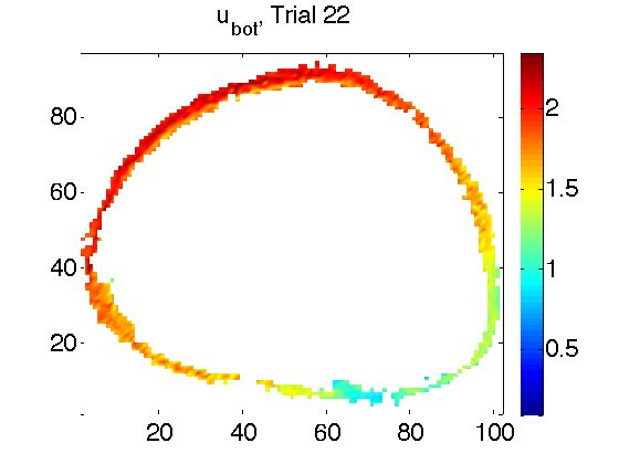
29(a) SWAN modeled ubot , Trial 22, depths: 10–20 m. (b) SWAN modeled ubot , Trial 23, depths: 10–20 m.
Figure 9: Extreme significant wave height events, Trials 22 and 23. Trial 22
features swell with Hsig = 9.2 traveling in a direction of 296◦ , whereas Trial 23
has swell with Hsig = 7.5 m/s traveling at 86◦ .
m/s (Trial 10). Trials 8, 9 and 10 also show elevated Tm01 ranges relative to Trial 1 and the θwind
trials. Additionally, the increases in Tm01 come from a 0.5 s increase in the lower range value for
every 1 m increase in boundary Hsig . The trials of increasing Hsig saw the lowest ranges for Fsaf ety
outside of the extreme events analysis. In the order of Trial 8, Trial 9, and Trial 10, the coral
species Fsaf ety ranges are: 500–1800, 250–1500 and 150–1200 for P. meandrina, 700–1100, 500–1100
and 400–1100 P. lobata, 200–1100, 150–900, and 100–700 for M. capitata and 1000-4500, 900–4000,
1900,6750 for P. compressa
Thus far, all the incoming waves discussed have come from the NW, at a direction of 295–315◦ and
have impacted the north and west of the atoll, generating spatial distributions relatively similar to
Fig 7. Trials 17–21 feature waves traveling at 105◦ , (headed north-northwest) and hitting the south
and east edges of the Atoll (Fig 9). Significant wave heights from Table 3 were run for this new wave
direction (Trials 17–20) because Hsig had the greatest influence over ubot . As with the ≈300◦ waves,
increasing Hsig at the boundaries caused increases in ubot and Tp , and the corresponding decreases
30(a) Factor of Safety: P. meandrina, Trial 22 (b) Factor of Safety: P. lobata, Trial 22
(c) Factor of Safety: M. capitata, Trial 22 (d) Factor of Safety: P. compressa, Trial 22
Figure 10: Extreme Event: Trial 22 Hsig = 19.2 m, Tp = 16 s, θ = 296◦ , wind
magnitude = 13.5 m/s and θwind = 139◦
in Fsaf ety values (Table 5). A slight difference between the 105◦ waves and the northwesterly swell is
that while 105◦ waves did not create as high of ubot ranges (see Trial 10 vs Trial 20), Trials 19 & 20
showed greater mean period ranges than their ≈300◦ counterparts. Coral factor of safety ranges were
similar to those in Trials 1 and 8–10, with better fitting on the lower end of the ranges, and, because
coral failure is one of the chief concerns of this project, the lower end of the range is the primary
concern when discussing Fsaf ety values. Finally, Trial 21, which had a significant wave height of 1.5
m but a period of 11 s, was run for 105◦ . The alterations to ubot , Tp and species-specific Fsaf ety
relative to the MCC condition for 105◦ (Trial 17) were similar to differences between Trials 11 and 1.
31You can also read